Hybrid Decision-Making using Adaptive Technology
Rodrigo Suzuki Okada
Escola Politécnica University of São Paulo
São Paulo, Brazil.
João José Neto
Escola Politécnica University of São Paulo
São Paulo, Brazil.
ABSTRACT
This paper presents a hybrid approach to decision-making, capable of calibrating a trade-off between accuracy and response time by using multiple decision-making techniques to reach a solution of a decision problem. Each device employed by the decision-making system should also be able to learn from solutions suggested by other devices. This can be achieved by applying adaptive techniques, which make possible to change each device’s behavior according to the input received. This process happens autonomously, without human interference.
General Terms
Decision Supporting Systems, adaptive technology, hybrid systems.
Keywords
Decision-making, adaptive device, case-based reasoning, Naive Bayes, k-Nearest Neighbors, decision table.
1.
INTRODUCTION
Decision-making is a reactive process, in which an action should be taken as a response to some external event, often determined by combining a set of criteria – also known as attributes [1]. Choosing the best alternative from a finite set of possible scenarios is a matter of gauging the possibilities and checking which ones are more attractive in a particular condition – commonly referred to as instance.
Decision-making problems are often found in a wide variety of fields, ranging from economics to medicine. Examples can be easily found even in everyday life – such as the choice of clothes according to the weather, or deciding what to cook for lunch, according to one’s own preferences.
One way to evaluate the performance of a decision-making method is by measuring its hit rate and the time needed to reach a satisfactory decision. Typically, hit rate and speed have an inverse relationship: spending more time analyzing a problem tends to yield higher hit rates. Yet, if the error cost is low, applying methods that sacrifice hit rate to achieve faster decisions may be a better choice. This relationship is shown in Fig 1.
Animals have shown to be able to perform a trade-off between speed and accuracy in order to maximize their gains [2]. Most of the computational decision-making methods, however, do not calibrate this trade-off, since they always use the same decision algorithm regardless of time or hit rate constraints.
The software architecture proposed in this paper representsa contribution towards a decision-model capable of calibrating a
[image:1.595.321.535.140.350.2]Speed-Accuracy Trade-off (SAT) by using different decision making methods according to their hit rate and response time.
Fig 1: Typical relationship between speed and accuracy for most decision tasks [2]. Easier tasks – illustrated by the
left curve – can be solved with high accuracy while retaining low response times.
2.
CONCEPTS
2.1
Decision Support System
The concept of Decision Support System first appeared in the 1970s as a computational artifact that aids decisional tasks [3], being originally employed by business organizations to achieve better strategic decisions.
Although there is no definitive model, most decision support systems combine a knowledge-based system with a decision model and a user interface, allowing the decision-maker to quickly compile useful information out of raw data [4].
Learning through training data is a classical method to build the system’s initial knowledge. Typically, learning is divided into two categories: eager learning and lazy learning: eager methods create a condensed representation during a learning phase by inferring abstractions from the training data, while lazy ones avoid abstracting until needed at runtime [5].
The structure of decision support systems has significantly evolved since its original concept, mostly because of the advent of computer intelligence, which increased their capabilities even further [3][6]. Their scope has also broadened, due to their inclusion in a wider range of fields, such as medical diagnosis and management.
One fundamental problem faced by decision support systems is maintainability: in order to work properly, their decision model and corresponding knowledge must be kept updated to minimize their miss rate. Particularly, concepts may change over time – an effect known as concept-drift [7]. If ignored, the system’s accuracy will degenerate as concepts change. Classical decision models, however, are immutable and need to be completely rebuilt from scratch to keep them up to date.
Evolutionary and adaptive systems – capable of acquiring new information without rebuilding the decision model from scratch and adapting themselves to their environment – are taken as a next step for decision support systems [8].
Response Time
Acc
u
ra
cy
Low High
High
Low Ac
cu
ra
cy
C
o
st
Speed Gain
Ac
cu
ra
cy
Ga
in
2.2
Rule-Driven Adaptive Devices
An adaptive device can be described as the union of usual devices – such as finite automata, grammars, decision trees and decision tables – and an adaptive mechanism, capable of changing the device’s behavior at runtime [9]. The device is often referred to as a subjacent device, while the action that modifies the device’s behavior is called adaptive action.
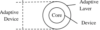
[image:2.595.80.254.207.260.2]As an example, the addition of an adaptive layer to a finite automaton may enable it to add and remove transitions, and generate new states as well. In fact, such automata are Turing-equivalent [10].
Fig 2: Structure for an adaptive device, composed of a rule-driven device and an external adaptive mechanism.
According to Neto [11], a rule-driven device (ND) is described as ND = (C, NR, S, c0, A, NA), where:
C is a set of possible configurations for ND, while c0∈C is the initial configuration.
S is a finite set of possible events that are valid input stimuli for ND. The null element ε is valid as well.
A ⊆ C is the subset of accepting configurations.
NA is a finite set of all possible symbols to be output by ND in response to the application of the rules in NR. Such output symbol may be interpreted as a procedure call, by mapping it into an action to be executed upon the application of a rule
NR ⊆C ×S ×C ×NA is a set of rules defining ND. The application of a rule r ∈ NR, denoted as r = (ci, s, cj, z), changes the current configuration ci into cj in response to a stimulus s ∈ S. As response, it outputs z ∈ NA.
An adaptive device AD, then, is described as ADk = (NDk, AM), where:
k ≥ 0 is a counter that is incremented by 1 whenever an adaptive action is taken.
NDk is the subjacent device after the execution of k adaptive actions. By this definition, ND0 is the initial subjacent device. ADk evolves to ADk+1 by executing an adaptive action. The evolved device will have a new set of rules NRk+1, consisting of an edited version of the previous NRk,
AM is the adaptive mechanism responsible for executing adaptive actions.
Expanding the previous definition into ADk = (Ck, ARk, S, ck, A, NA, BA, AA):
Ck is a set of possible configurations for ADk, while ck∈Ck is the initial configuration at step k. At k=0, this set is the same as the one defined for ND.
S, A and NA retain their former meanings.
BA and AA are sets of adaptive actions that should happen, respectively, before and after applying a rule. Both should contain the null action, which does not trigger any adaptive action (ε ∈ BA ∩ AA).
The set of rules of an adaptive device has been renamed to ARk⊆ BA×C ×S ×C ×NA ×AA. Adaptive rules have the form ark = (ba, ci, s, cj, z, aa). When applied, this rule initially executes the adaptive action ba ∈ BA. Then, the subjacent non-adaptive rule in form of (ci, s, cj, z) is executed. Finally, it executes the adaptive action aa ∈ AA. In the case that aa = ba = ε, the rule is essentially non-adaptive.
Algorithm 1 sketches the overall operation of an adaptive device AD. It is, basically, a loop that iterates over the elements of an input stream w, extracting its input symbols scurrent, one at a time, and using each of them to find and execute a set of matching rules CRT. Matching rules are ones whose configuration ci and input symbol s match the device’s current configuration ccurrent and the input symbol scurrent respectively. This search scheme is outlined in Algorithm 2. Formally, the set of matching rules is defined as CRT = {ar ∈ ART | ar = (ba, ci, s, cj, z, aa), ci = ccurrent, s ∈ {scurrent, ε}; ci,cj∈ CT; ba ∈ BA; aa ∈ AA, z ∈ NA}.
Algorithm 1 runRuleDrivenDevice(AD, w, out)
Input
AD: Device to be executed w: Input stream of symbols s ∈ S
Output
out: Output stream of symbols z ∈NA 1. set AD.ccurrent c0
2. for each scurrentin w do 3. consumed false 4. while not consumed do
5. CRT searchRules(AD, scurrent) 6. if CRT = ∅then
7. reject w
8. else if | CRT | = 1 then
9. ar single element of CRT 10. consumed executeD(AD, ar, out)
11. else
12. consumed executeND(AD, CRT , out)
13. end if
14. end while
15. end for
16. if AD.ccurrent∈ AD.A then 17. accept w
18. else
19. reject w 20. end if
The execution of CRT depends on its own cardinality. If the search yields only one rule (i.e., |CRT | = 1), it can be deterministically applied, consuming the input symbol read, writing z to the output stream and updating the device’s current configuration to cj. If the rule specifies non-empty adaptive actions ba and/or aa, they should be executed as well. However, the execution is aborted if ba eliminates the current rule from ARk – in this case, the device should find another set of matching rules to execute. This operation is described in Algorithm 3.
Core
Adaptive Layer
Device Adaptive
Algorithm 2 searchRules(AD, s)
Input
AD: Device to be executed
s: Symbol s ∈ S read from the input stream
Output
Set of matching rules CRT
1. CRT { }
2. for each ar = (ba, ci, s, cj, z, aa) ∈ AD.ART do 3. if (ar.ci, ar.s,) = (AD.ccurrent , s) then 4. add ar to CRT
5. end if
6. end for
7. return CRT
Algorithm 3 executeD(AD, ar, out)
Input
AD: Rule-Driven Adaptive Device to be executed ar: Rule to be executed
Output
out: Output stream of symbols z ∈ NA 1. if ar.ba ≠ ε then
2. adapt(AD, ar.ba) 3. end if
4. if ar AD ∉AR then
5. return false 6. end if
7. AD.ccurrent ar.cj 8. append ar.z to out 9. if ar.aa ≠ ε then
10. adapt(AD, ar.aa) 11. end if
12. return true
However, if |CRT | = m ≥ 1, multiple rules are equally allowed to be executed. In this case, they should be non-deterministically applied to the current configuration – which is usually simulated in non-parallel environments by using some backtracking strategy. This featured is performed by the executeND function in Algorithm 1.
Note: the execution of non-deterministic scenarios is voided in this work, by keeping it purely deterministic. Case studies for particular adaptive devices, such as non-determinism in decision-trees, have been addressed in previous works [12][13].
Finally, if |CRT | = 0, then no rule can be applied to the current configuration using s. In this case, the input stream w is rejected.
Once all symbols have been consumed, the input stream w is accepted if the ending configuration is member of A – i.e., ccurrent∈ A – otherwise, w is rejected
2.3
Extended Adaptive Decision Tables
Decision table is a popular rule-driven device employed to solve decision-making problems. Typically, decision tables make use of a set of rules represented by a condition and a corresponding action to be taken when the condition applies to the problem being solved. Conditions usually have binary entries as valid values, although it is possible to extend this concept to an arbitrary number of discrete values – tables employing this kind of condition are known as extended entry decision-tables.
Classical decision tables have static rules, which are all predefined and cannot change throughout the device’s operation. Moreover, the set of rules itself is immutable, and do not support the inclusion or exclusion of rules.
[image:3.595.53.282.68.441.2]Adaptive Decision Tables (ADT), according to the definition given in Section 2.2, join a classical decision table and an adaptive layer, which contains a set of actions to be taken before and after a rule is applied. Each action is formed by a list of elementary actions of type query, insertion and exclusion, responsible for each basic change to be made to the set of rules.
Fig 3: Scheme of an Extended Adaptive Decision Table and its auxiliary method, as seen in [14].
Tchemra has further expanded ADT’s adaptive capability by adding auxiliary functions that are called when no matching rules can be found [14]. This way, rather the rejecting an input, the device will try to create a new matching rule for the current situation, allowing it to proceed. The resulting formalism has been named Extended Adaptive Decision Table (EADT).
Creation of new rules is achieved by means of a second device – named auxiliary method – to return a solution, which is incrementally added to the set of existing rules. One possibility studied in [14] was Analytic Hierarchy Process (AHP), which solves the problem by comparing alternatives through a score matrix, which describes the performance of all alternatives according to each criterion.
It’s worth noting that EADT, although focused on the decision table itself, represents a hybrid approach to decision making by using different kinds of devices to solve a decision problem. This constitutes an important contribution, since this scheme allows incremental learning, which keeps the primary device – the decision table – updated with the help of another device to solve problems out of scope of the primary one.
This concept can be extended to the general adaptive device by replacing line 7 of Algorithm 1 with the following pseudo-code:
…
7. adaptFM(device, s) ...
Call Auxiliary Method
Decision Table
Adaptive Functions
Auxiliary Functions
AHP (Analytic Hierarchy Process)
Decision Problem
Solution
No rule found Execute adaptive
function Adapt rules
[image:3.595.325.547.201.403.2]where adaptFM(device, s) is the auxiliary function that should call the secondary device, and create a new rule based on its response.
3.
HYBRID DECISION-MAKING
3.1
Definitions
According to the definition used in most Instance-Based Learning methods, the term instance means a set a set of values, which describes the problem to be solved. Each value represents the state of a single criterion to be measured. Internally, each instance k is represented as an m-dimensional vector xk, where the i-th component represents the value of the i-th criterion.
k k ki km
k
x
x
x
x
x
1,
2,...,
,...,
(1)For continuous criteria, values must be numeric, while nominal categories make use of literal names as values – out of a finite set of allowed names.
Then, using this definition, a decision-making device must be able to analyze an input instance xk and solve it by outputting an alternative yk.
kk
solve
x
y
(2)3.2
Proposition
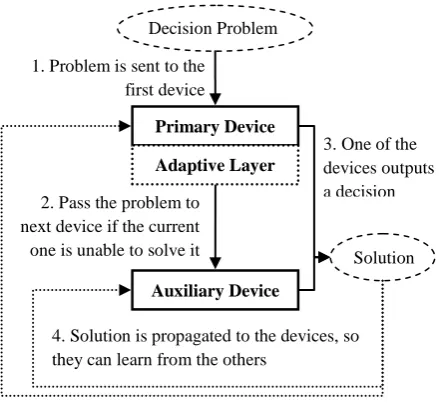
[image:4.595.61.281.408.610.2]Based on the premise that perceptually easier tasks can be quickly solved without having to sacrifice significant amounts of accuracy, a hybrid decision-making environment may be able to reduce time consumption by assigning easier problems to faster devices – which are supposed to be less accurate – while using slower devices to solve harder problems.
Fig 4: Generalization of EADT’s hybrid decision-making process to any kind of devices.
For this purpose, EADT’s hybrid approach is extended to make it possible to use other kinds of devices rather than the original ones (decision tables and AHP). Those devices should be sorted by their response time – the faster ones should be placed first. When solving a problem, this hybrid environment assigns it to the first device in the queue – the faster one. If the device is able to solve it, the decision should be outputted, otherwise, the problem is assigned to the auxiliary device. Once a decision is made, it is propagated to both devices, which, in turn, can incorporate the new
knowledge to assist future decisions. This process is shown in Fig 4.
For rule-driven devices such as decision tables and decision trees, solving a problem means that there is some rule that applies to it. However, methods such as Naive Bayes and k-Nearest Neighbor are based on probabilities rather than rules, making it hard to identify whether a proper solution has been achieved or not.
For probabilistic-based methods, one possible way to determine whether a solution is acceptable or not is by analyzing the class distribution – i.e., the probability of each alternative being a solution – and accept the most probable alternative i, as long its probability pi is over a certain threshold.
p p p thresh
accept max 1, 2,..., n (3)
Taking condition (3), the decision-making device’s operation is described in Algorithm 4, where p is the class distribution, pi is the highest probability found, and ai is its corresponding alternative. The first call to this function must have k=0.
Algorithm 4 makeDecision(D, k, x, y, t, P)
Input
D: List of devices to be executed k: Index of the device to be executed now x: Input instance
t: Threshold for accepting the solution
Output
y: Output alternative
P: Class probability for each device 1. p D[k].getProbabilities(x) 2. append p to P
3. pi max(p) 4. if (pi > t) then
5. y ai
6. else if (k+1 < D.length) then
7. makeDecision(D, k+1, x, y, t, P) 8. else
9. makeDecisionLast(D, x, y, P) 10. end if
Algorithm 5 makeDecisionLast(D, x, y, P)
Input
D: List of devices to be executed x: Input instance
Output
y: Output alternative
P: Class probability for each device 1. p D[D.lastElement].getProbabilities(x) 2. i index of max(p)
3. y ai
Additionally, the function getProbabilities should be implemented according to the devices being used. Lines 3 and 4 show the condition represented by equation (3).
A strategy must be chosen when no device can solve the problem. The simplest one is to just return a void solution. If the problem demands a non-void solution, arbitrary actions could be chosen, such as returning the latest device’s decision, or choosing by vote among all devices. That action is performed by the makeDecisionLast function at line 9. As an example, in order to return the latest device’s decision, this 2. Pass the problem to
next device if the current one is unable to solve it
Primary Device
Adaptive Layer
Decision Problem
Solution
Auxiliary Device
1. Problem is sent to the first device
4. Solution is propagated to the devices, so they can learn from the others
function can be implemented by Algorithm 5. This is the strategy applied in this work.
Finally, the decision outputted by Algorithm 4 should be propagated to all devices, allowing them to learn one from another. This is illustrated in Algorithm 6. The learn function is device-dependent, and should be implemented accordingly.
Algorithm 6 learningPhase(D, x, y)
Input
D: List of devices to be executed x: Input instance
y: Solution given by makeDecision() 1. for each d in D do
2. d.learn(x, y) 3. end for
4.
EXPERIMENTAL SYSTEM
The presented decision-making environment was tested by creating a sample system, composed of two decision-making devices, the first one being a Naive Bayes classifier– i.e., the fastest one. Problems whose solution do not satisfy equation (3) will, then, be solved by the second device, a k-Nearest Neighbor classifier – which, being instance-based, is considerably slower, especially for large datasets.
Their integration of those classifiers within the proposed decision-making environment is described below.
4.1
Naive Bayes
Naive Bayes is a simple classifier which assumes that each criterion have an independent contribution to the probability of each possible solution to a problem. According to the Bayes' Theorem, the probability of an instance xa to have alternative c as solution is given by:
m i ai aa pc px c
x Z x c p 1 | 1 | (4)
where p(c) is a priori probability of c being a solution to any instance, while p(xai|c) is the probability of the i-th criterion having xai as value when c is a correct solution. This equation should apply for each alternative – the resulting set of probabilities should be returned by the getProbabilities function in Algorithm 5.
The value Z refers to the evidence, which normalizes the probability:
n j m i j ai ja pc px c
x Z
1 1
| (5)
The p(c) value can be estimated by checking the probability of alternative c being a solution to any instance. Then:
n j s i j i s i i c x f I c x f I c p 1 1 1 (6)where I(z) is the indicator function, returning 1 if the condition z is true, otherwise, returning 0. The function f(x) returns the alternative of the instance x – this information is usually stored in a database. As for p(xai|c), it can be estimated in a similar fashion, by counting how many times the value xai appears when alternative c is a solution:
s j j s j ai ji j ai c x f I x x I c x f I c x p 1 1 | (7)However, in order to work properly, the instances’ values must be discrete, while previous definitions state that values may be continuous, numeric values. This is usually solved by discretizing numeric values into discrete ones using some particular scheme. For this work, we’ll use Equal Width Discretization with 100 steps of equal width, as defined in [15].
Finally, it’s worth noting that, although the previous equations depend on an iteration of all instances, their calculation can be done more efficiently by storing the values for the sums of:
s j j c x f I c s 1 (8) and:
s j ji j c I x vx f I v i c s 1 . , (9)
for each alternative c, criterion i and a possible value v.
During the learning stage described in Algorithm 6, Bayes can incorporate new knowledge by storing a new instance xh and its corresponding alternative y=f(xh) in a database, and then, updating sums (8) and (9).
This process, however, assumes that f(xh) has not been set beforehand. A strategy should be adopted if the device receives an instance with a previously set alternative:
One possibility is to ignore the new information altogether, keeping the current f(xh);
Another one is to overwrite the previous alternative. The sums should be updated by removing the previous contributions of f(xh) from the sums and adding the new ones.
This problem is further explored in sections 5 and 6.
4.2
k-Nearest Neighbor
The k-Nearest Neighbor – commonly referred as k-NN – is a popular instance-based classifier that estimates a classification of a new instance by searching for similar instances, and uses the k-nearest ones to vote the new instance’s solution. The original k-NN is defined as in [16]:
k i i c c cnew I f x c
y
n} 1' ... { ) ( argmax 1 (10)
where f(xi) is the alternative of a nearby instance xi. A common extension to this definition is the addition of a weighting function based on the similarity between the new instance and the nearest ones – closer instances should receive higher weight:
) ( , ) ( argmax 1 } ... {1 i new k i i c c cnew I f x c w x x
y n
(11)where w(xnew, xi) is the weighting function. Then, the probability of alternative c being a solution to xa is:
t a
ak
i
i
a I f x c w x x Z x
x c
p | ( ) ( , )
1
(12)
n
j
a t k
i
j i
a I f x c wx x
x Z
1 1
) , ( )
( (13)
For the weighting function, one possibility is to use Shepard’s method [17]:
p b a b a
x x d x x w
) , (
1 ) ,
( (14)
where P is a positive scale value – in this work, P=2 – while d(xa, xb) is a distance function that calculates the difference between two instances by checking the individual differences between their criteria’s values – the difference in the j-th criterion is denoted by dj(xa, xb), which should return values in the 0…1 range for normalization purposes.
m x x d
x x d
m
j j
1
2 2 1
2 1
) , (
) ,
( (15)
For numeric criteria, the difference is the usual Euclidean one, although normalized by dj max, which is the maximum difference possible for such criterion.
max 2 1 2 1, )
( j j j
j x x x x d
d (16)
For nominal, discrete values, however, the concept of distance becomes less clear. A simple, fast solution is the Overlap Metric (OM) [18]:
) , ( ) ,
( 1 2 1j 2j
j x x x x
d
(17)where δ(x1j, x2j) is a function that returns 0 if x1j = x2j, returning 1 otherwise. Another option is the Value Difference Metric (VDM) [18], which uses additional information about how the values are related to the alternatives. Its definition is:
C
c
j j
j x x P c x Pc x
d
1
2 1
2
1, ) ( | ) ( | )
( (18)
where P(c | xij) is the probability of the instance xi having c as alternative, given that its j-th criterion has the value xij. This is estimated by counting how many times each alternative appears when an instance has the xij value when compared to the others. Albeit slower, VDM allows for an overall better hit rate.
For the learning phase, since k-NN does not store any abstraction out of the raw data, just storing the values x and their corresponding f(x) in a typical database is enough. The need of a strategy for cases of overwriting older data – discussed at the end of section 4.1 – still stands, though.
Finally, it’s important to note that the k-NN’s response time greatly depends on the search method – this study makes use of a linear search. For practical purposes, however, making use of a spatial indexed search is preferable.
5.
RESULTS
5.1
Speed-Accuracy Trade-Off
The experimental system was tested through datasets provided by the UCI Machine Learning Repository [19]. In order to check how the threshold in (3) affects the hit rate and response time, each dataset has been tested with thresholds ranging from 0.3 to 1.0, in steps of 0.02. At each step, 50 consecutives tests have been run, using 70% of the data for training, while using the remaining 30% as input to measure the hit rate. If neither devices are able to return an alternative
that satisfies (3), the last device’s decision – the k-NN`s – will prevail, as described in Algorithm 6.
The k-NN algorithm has been set to use a fixed k=10, while using Shepard`s method to calculates weights, using P=2. Differences between numeric values were calculated using (16), while using VDM for nominal ones, as shown in (18).
For the learning phase, there’s the need of some strategy to apply when the learn function receives an already known instance, but initialized with another alternative – as explained in section 4.1. Assuming that the initial training data is more likely to be error-free, the first strategy will be applied, so new solutions – more prone to errors – will not overwrite older ones.
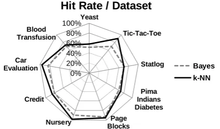
While slower, k-NN attains higher hit rates than Bayes on most of the datasets tested – as shown in Fig 5. On average, the difference was 7%. Statlog is the only dataset whose k-NN’s hit rate was lower than Bayes’ (a difference of 0.65%).
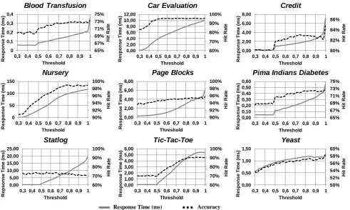
The impact of the threshold on the hit rate and response time is displayed in Fig 6. The response time, as expected, increases as the threshold increases, since this means more problems are being solved by k-NN. The response time’s order of magnitude is heavily influenced by the dataset’s size, since k-NN becomes slower as the dataset grows bigger – Nursery has almost 13000 instances, while the Blood Transfusion has only 748.
Note: some datasets show no changes until threshold is over 0.5. That happens on datasets with just two alternatives – in this case, the most likely alternative’s score is never below 0.5.
0% 20% 40% 60% 80% 100%Yeast
Tic-Tac-Toe
Statlog
Pima Indians Diabetes Page
Blocks Nursery
Credit Car Evaluation
Blood Transfusion
Hit Rate / Dataset
[image:6.595.313.538.412.544.2]Bayes k-NN
Fig 5: Hit rate for 9 UCI Datasets, using Naive-Bayes and k-Nearest Neighbor.
However, the behavior of the hit rate varies among datasets. Generally, the hit rate increases rather proportionally to the response time, making it possible to adjust the trade-off between speed and hit rate by moving the threshold – e.g., if it was required to solve the Pima Indians Diabetes in an average of 0.2ms per problem, choosing a threshold of 0.7 would maximize the hit rate under this constraint.
Fig 6: Effects of the threshold on the hit rate and the response time. 65% 67% 69% 71% 73% 75% 0 0,1 0,2 0,3 0,4
0,3 0,4 0,5 0,6 0,7 0,8 0,9 1
H it R a te R e s p o n s e T im e ( m s ) Threshold
Blood Transfusion
60% 70% 80% 90% 100% 0,00 2,00 4,00 6,00 8,00 10,00 12,00
0,3 0,4 0,5 0,6 0,7 0,8 0,9 1
H it R a te R e s p o n s e T im e ( m s ) Threshold
Car Evaluation
80% 82% 84% 86% 0,00 2,00 4,00 6,00 8,000,3 0,4 0,5 0,6 0,7 0,8 0,9 1
H it R a te R e s p o n s e T im e ( m s ) Threshold
Credit
90% 92% 94% 96% 98% 100% 0 50 100 1500,3 0,4 0,5 0,6 0,7 0,8 0,9 1
H it R a te R e s p o n s e T im e ( m s ) Threshold
Nursery
90% 92% 94% 96% 98% 100% 0,00 2,00 4,00 6,00 8,000,3 0,4 0,5 0,6 0,7 0,8 0,9 1
H ir R a te R e s p o n s e T im e ( m s ) Threshold
Page Blocks
65% 67% 69% 71% 73% 75% 0,00 0,10 0,20 0,30 0,40 0,50 0,600,3 0,4 0,5 0,6 0,7 0,8 0,9 1
H it R a te R e s p o n s e T im e ( m s ) Threshold
Pima Indians Diabetes
60% 70% 80% 90% 100% 0,00 5,00 10,00 15,00 20,00 25,00
0,3 0,4 0,5 0,6 0,7 0,8 0,9 1
H it R a te R e p s o n s e T im e ( m s ) Threshold
Statlog
60% 70% 80% 90% 100% 0,00 1,00 2,00 3,00 4,00 5,00 6,000,3 0,4 0,5 0,6 0,7 0,8 0,9 1
H it R a te R e s p o n s e T im e ( m s ) Threshold
Tic-Tac-Toe
50% 52% 54% 56% 58% 60% 0,00 0,50 1,00 1,500,3 0,4 0,5 0,6 0,7 0,8 0,9 1
H it R a te R e s p o n s e T im e ( m s ) Threshold
Yeast
Response Time (ms) Accuracy
Finally, since k-NN had a worse performance than Bayes for the Statlog dataset, there was no advantage in using this hybrid approach, since shifting more problems to k-NN actually made the system less accurate and more time-consuming.
5.2
Comparison to Greedy Solving
In order to check the gains of using the experimental hybrid system when compared to a greedy approach, we have implemented a simple system that solves as many problems with k-NN as possible. However, once the average response time goes over a certain time threshold, it starts to use Bayes until the average drops below the threshold, then switching back to k-NN. The final average should be close to the time threshold established. Such system, differently from the experimental one, has no criteria for choosing which device should be used.
50% 60% 70% 80% 90% 100%
Blood Transfusion Car Evaluation Credit Nuersery Page Blocks Pima Indians Diabetes Statlog Tic-Tac-Toe Yeast
Accuracy / Dataset
Greedy Hierarchical
Fig 7: Comparison between our system and a greedy one.
The accuracy of this greedy system was measured using a time threshold equal to the average response time from the previous experiment at threshold 0.6 – e.g., for the Nursery and Yeast datasets, the time thresholds were 50ms and 1ms respectively.
When compared to this greedy system, the accuracy obtained with the experimental one – with threshold=0.6 – was, on average, 2% higher, beating it in 8 out of 9 datasets. The gap was larger on datasets whose difference in accuracy between k-NN and Bayes was larger, such as Car Evaluation and Tic-Tac-Toe.
6.
CONCLUSION AND FUTURE WORK
This work introduced a hybrid decision-making method that operates with the help of adaptive techniques. The proposed system allows calibrating the trade-off between hit rate and response time by choosing an appropriate threshold. Additionally, it was shown that it is possible to achieve a hit rate close to the most accurate device’s own hit rate, although consuming just part of its original response time.
One aspect to be explored further is the strategy to adopt when the information to be learnt conflicts with previously known stored ones – as described in section 4.1. Rather than just ignoring the new information or completely overwriting the older one, one possibility to be studied is the use of characteristic functions rather than indicators functions [20]. That would allow an instance to have multiple solutions with different degrees of strength. Rather than handling the crisp f(x) function, the learn function would pamper a membership function, making it more flexible to changes.
[image:7.595.57.275.573.734.2]7.
REFERENCES
[1] Crozier, R. and Ranyard, R. 1997. Cognitive process models and explanations of decision making. In Decision Making, Cognitive Models and Explanations, 5-20.
[2] Chittka, L., Skorupski, P. and Raine, N. E. 2009. Speed-Accuracy Tradeoffs in Animal Decision Making. Trends in Ecology & Evolution, Vol.24, No.7, 400–407.
[3] Sol, H. G., Takkenberg, C. A. T. and Robbé, P. F. V. 1985. Expert Systems and Artificial Intelligence in Decision Support Systems. In Proceedings of the Second Mini Euroconference. 17-20.
[4] Sprague, R. H. and Carlson, E. D. 1982. Building Effective Decision Support Systems. Englewood Cliffs: Prentice Hall Professional Technical Reference. 30-32.
[5] Hendrickx, I. and Bosch, A. 2005. Hybrid Algorithms with Instant-Based Classification. In Machine learning - ECML 2005, 158-169.
[6] Bui, T. and Lee, J. 2003. An Agent-Based Framework for Building Decision Support Systems. Decision Support Systems, Vol.25, No.3, 225-237.
[7] Kuncheva, L. I. 2009. Using Control Charts for Detecting Concept Change in Streaming Data. Technical Report. Bangor University.
[8] Arnott, D. 2004. Decision Support Systems Evolution: Framework, Case Study and Research Agenda. European Journal of Information Systems, Vol.13, No.4, 247-259.
[9] Pistori, H. 2003. Tecnologia Adaptativa em Engenharia de Computação: Estado da Arte e Aplicações. Doctoral Thesis. EPUSP (in Portuguese).
[10]Rocha, R. L. A. and Neto, J. J. 2000. Autômato adaptativo, limites e complexidade em comparação com máquina de Turing. In Proceedings of the second Congress of Logic Applied to Technology – LAPTEC 2000. 33-48 (in Portuguese).
[11]Neto, J. J. 2002. Adaptive Rule-Driven Devices - General Formulation and Case Study. Lecture Notes in Computer Science, Vol.2494. 466-470.
[12]Castro Jr., A. A., Neto, J. J. and Pistori, H. 2007. Determinismo em Autômatos de Estados Finitos Adaptativos. Revista IEEE América Latina, Vol.5, No.7, 515-521 (in Portuguese).
[13]Pistori, H., Neto, J. J. and Pereira, M. C. Adaptive Non-Deterministic Decision Trees: General Formulation and Case Study. INFOCOMP Journal of Computer Science, 2006, in press (in Portuguese).
[14]Tchemra, A. H. 2009. Tabela de Decisão Adaptativa na Tomada de Decisão Multicritério. Doctoral Thesis. EPUSP (in Portuguese).
[15]Yang, Y. and Webb, G. I. 2002. A Comparative Study of Discretization Methods for Naive-Bayes Classifiers. In Proceedings of PKAW 2002: The 2002 Pacific Rim Knowledge Acquisition Workshop. 159-173.
[16]Liu, W. and Chawla, S. 2011. Class Confidence Weighted kNN Algorithms for Imbalanced Data Sets. In Proceedings of the 15th Pacific-Asia Conference on Advances in Knowledge Discovery and Data Mining. 345-356.
[17]Shepard, D. 1968. A Two-Dimensional Interpolation Function for Irregularly-Spaced Data. In Proceedings of the 1968 ACM National Conference. 517-524.
[18]Li, C. and Li, H. 2010. A Survey of Distance Metrics for Nominal Attributes. Journal of Software, Vol.5, No.11, 1262-1269.
[19]Frank, A. and Asuncion, A. 2010. UCI Machine Learning Repository. Irvine, CA: University of California, School of Information and Computer Science. http://archive.ics.uci.edu/ml.
![Fig 1: Typical relationship between speed and accuracy for most decision tasks [2]. Easier tasks – illustrated by the](https://thumb-us.123doks.com/thumbv2/123dok_us/8115937.792500/1.595.321.535.140.350/typical-relationship-speed-accuracy-decision-tasks-easier-illustrated.webp)
![Fig 3: Scheme of an Extended Adaptive Decision Table and its auxiliary method, as seen in [14]](https://thumb-us.123doks.com/thumbv2/123dok_us/8115937.792500/3.595.325.547.201.403/fig-scheme-extended-adaptive-decision-table-auxiliary-method.webp)