Boundary Value Problem for the System Equations Mixed Type

Boundary Value Problem for the System Equations

Mixed Type

Fayazov K.S.

,

Khajiev I.O.

∗

Mathematics Faculty, National University of Uzbekistan, Universitet Str. 4, 100174 Tashkent, Uzbekistan

Copyright c2016 by authors, all rights reserved. Authors agree that this article remains permanently open access under the terms of the Creative Commons Attribution License 4.0 International License

Abstract

In this paper, we consider a system of equations of mixed type and with changing time direction. It is proved that solution of the system is not stable depend from the vari-ation of the data. Theorems of uniqueness and conditional stability proved. The approximate solution constructed and numerical results are given.

Keywords

System of Equations, Boundary Value Prob-lem, Ill-posed ProbProb-lem, a Priori Estimate, Theorem of the Uniqueness, Estimate of Conditional Stability, Approximate Solution, Regularization, Regularization’s Parameter

1

Introduction

Consider the system of equations 





signx∂2 ∂t2 +

∂2 ∂x2

v(x, t) = 0,

signx_∂t∂ +_∂x∂22

u(x, t) =v(x, t) (1)

on the domainΩ ={−1< x <1, x6= 0, 0< t < T}.

Problem. Find a solution(u(x, t), v(x, t))of the system equations (1), satisfying the initial

u(x,0) =f(x),

v(x,0) =g(x), vt(x,0) =h(x)

, −1≤x≤1, (2) the boundary conditions

u(−1, t) =u(1, t) = 0, v(−1, t) =v(1, t) = 0

, 0≤t≤T, (3) and the gluing conditions

u(−0, t) =u(+0, t), ux(−0, t) =ux(+0, t),

v(−0, t) =v(+0, t), vx(−0, t) =vx(+0, t)

   

  

, 0≤t≤T. (4)

The investigate problem belongs to the class of ill-posed problems of mathematical physics. Correct problems for such equations considered by M. Gevrey, D. Pagani, G. Tal-enti, V. N. Vragov, V. K. Romanko, A.M. Nakhushev and

others. See also works of N.V. Kislov, S. G. Pyatkov, A. I. Kozhanov, I.E. Egorov, A.A. Kerefov, I.S. Pulkin [1] and others.

The most important example of such type equations are mixed-type equation. A systematic study of them began with the work F.Tricomi and S. Gellerstedt. Shortly because of research S.A. Chaplygin and F.I. Frankl found out that mixed-type equations have important practical applications in the calculation of the flow of gas at around and super-sonic speeds. Many important practical applications, such as jet aircraft and astronautics, rocketry, gas-dynamic lasers, caused an avalanche growth in boundary value problems of research for equations of mixed type, as a purely mathemati-cal, and having applied nature.

Ill-posed problems investigated by H. Levine [2], A.L. Bukhgeim, K.S. Fayazov [5] and others.

In this paper we study the conditional correctness, prove the theorem on conditional stability and uniqueness of the solution of problem (1) - (4) and construct an approximate solution by the regularization method. We estimate norm of the difference between exact and regularized solutions.

Definition. By solution of the problem (1)-(4) we under-stand a pair of functions(u, v)having respective continuous derivatives involved in the system of equations and satisfy the system of equations (1) and the conditions (2) - (4).

2

The main results

For further discussion, we need in the following lemmas:

Lemma 1[6].Letv(x, t)satisfies the equation

sign x vtt(x, t) +vxx(x, t) = 0

and conditions v(−1, t) = v(1, t) = 0, v(−0, t) =

v(+0, t), vx(−0, t) = vx(+0, t),then forv(x, t)for every

0< t < T the following estimate

kv(x, t)k2≤2kv(x,0)k2+p

T−t T

kv(x, T)k2+p

t T

e2t(T−t),

is true, wherep=1 2

kvxx(x,0)k 2

+kvt(x,0)k 2

.

Lemma 2.Letu(x, t)satisfies the equation

sign x ut(x, t) +uxx(x, t) =v(x, t) (5)

and conditions u(−1, t) = u(1, t) = 0, u(−0, t) =

u(+0, t), ux(−0, t) =ux(+0, t),then foru(x, t)for every

0< t < T the following estimate

ku(x, t)k2≤2 ku(x,0)k2+

Z T

0

kv(x, t)k2dt !TT−t

×

ku(x, T)k2+

Z T

0

kv(x, t)k2dt !Tt

+

Z T

0

kv(x, t)k2dt,

is valid.

Proof.Solution of the equation (5) one can present as the sum

u(x, t) = ¯u(x, t) + ˜u(x, t), whereu¯(x, t)solution of the homogeneous equation

signxu¯t(x, t) + ¯uxx(x, t) = 0,

˜

u(x, t)- a particular solution of the inhomogeneous equation signxu˜t(x, t) + ˜uxx(x, t) =v(x, t).

Moreover functionsu¯(x, t),u˜(x, t)satisfy the boundary con-ditions

¯

u(−1, t) = ¯u(1, t) = 0, u˜(−1, t) = ˜u(1, t) = 0,

and gluing conditions

¯

u(−0, t) = ¯u(+0, t), u¯x(−0, t) = ¯ux(+0, t),

˜

u(−0, t) = ˜u(+0, t), u˜x(−0, t) = ˜ux(+0, t).

According to the results of [5, 6] solutionsu¯(x, t)andu˜(x, t)

can be presented in the form

¯

u(x, t) =

∞

X

k=1

¯

u+_k(t)X_k+(x) +

∞

X

k=1

¯

u−_k(t)X_k−(x),

˜

u(x, t) =

∞

X

k=1

˜

u+_k(t)X_k+(x) +

∞

X

k=1

˜

u−_k(t)X_k−(x),

hereu¯±_k(t),u˜±_k(t)for eachk= 1,2, ...satisfy the following problems, respectively:

˜

u+_k(t) _t−λ+_ku˜+_k(t) =v_k+(t),

˜

u+_k(0) =−RT

0 e

−λ+_kτ_v+ k(τ)dτ ,

˜

u−_k(t) _t−λ−_ku˜−_k(t) =v_k−(t),

˜

u−_k(0) = 0, and

¯

u+_k(t) _t−λ+_ku¯+_k(t) = 0,

¯

u_k+(0) =f_k++R₀Te−λ+kτv+

k(τ)dτ ,

¯

u−_k(t)

t−λ

−

ku¯

−

k(t) = 0,

¯

u−_k(0) =f_k−,

where v±_k(t) = R1

−1signx v(x, t)X

±

k(x)dx, f

±

k =

R1

−1signx f(x)X

±

k(x)dx, X

±

k(x)- eigenfunctions,

corre-sponding respectively to positiveλ+_k and negativeλ−_k eigen-values, and numbersλ+_k,−λ−_k constitute non-decreasing se-quence. Notice, that X_k±(x) and λ±_k eigenfunctions and

eigenvalues of the following problem: 

  

  

signx X00(x) +λ X(x) = 0, X(−1) = 0, X(1) = 0, X(−0) =X(+0), X0(−0) =X0(+0).

It is easy to note [3], that

˜

u+_k(t) =− Z T

t

eλ+k(t−τ)_v+

k(τ)dτ ,

˜

u−_k(t) =

Z t

0

eλ−k(t−τ)v−

k(τ)dτ ,

from here you can get

ku˜(x, t)k2=

∞

X

k=1

˜

u+_k(t) 2+

˜

u−_k(t) 2≤

Z T

0

kv(x, t)k2dt. (6)

Next, using the logarithmic convexity of the functionsu¯±_k(t)

for eachk= 1,2, ..., we have the following estimates

¯

u+_k(t) 2≤

¯

u+_k(0) 2

T−t T

¯

u+_k(T) 2

t T

,

¯

u−_k(t) 2≤

¯

u−_k(0) 2

T−t T

¯

u−_k(T) 2

t T

.

Summing overk,k= 1, 2, ...and using the Holder inequal-ity for the sum we have

ku¯(x, t)k2≤2ku¯(x,0)k2

T−t T

ku¯(x, T)k2

t T

,

and thatu¯(x, t) =u(x, t)−u˜(x, t), then

ku(x, t)k2≤2ku(x,0)k2+ku˜(x,0)k2

T−t T

×

ku(x, T)k2+ku˜(x, T)k2

t T

+ku˜(x, t)k2,

taking into account (6) from this we obtain required inequal-ity. The Lemma 2 proved.

Set of correctness M is defined as follows

M =n(u, v) :ku(x, T)k2+kv(x, T)k2≤m2o. (7)

Theorem 1.Let the solution of the problem (1) - (4) exists and(u(x, t), v(x, t))∈M, then the solution of the problem is unique.

Proof. Let two pair of functions (u1(x, t), v1(x, t)),

(u2(x, t), v2(x, t))are solutions of problem (1) - (4). We

denoteu(x, t) = u1(x, t)−u2(x, t), v(x, t) = v1(x, t)−

v2(x, t). Then pair of functions (u(x, t), v(x, t)) satisfies

the system of equations (1) and the homogeneous condi-tions (2) - (4). From the result of Lemma 1 it is easy to see kv(x, t)k = 0thenv(x, t) = 0, and on the base of Lemma 2, we get ku(x, t)k = 0, from here u(x, t) = 0 for any

(x, t) ∈Ω. Thenv1(x, t) ≡v2(x, t), u1(x, t)≡ u2(x, t),

solution of problem (1) - (4) is unique. The theorem proved.

kg(x)−gε(x)kW2

2 ≤ε,kh(x)−hε(x)k ≤ ε. Then the so-lution of problem (1) - (4) for everyt ∈ (0, T)satisfies the inequalities

kv(x, t)k2≤2 2ε2TT−t _m2_+ε2Tt_e2t(T−t)_,

ku(x, t)k2≤2 ε2+γ(m, ε)TT−t _m2_{+γ(m, ε)}Tt_{+γ(m, ε),}

whereγ(m, ε) = 2R₀T 2ε2

T−t

T _m2_+ε2Tt_e2t(T−t)_dt.

Proof. On the base of the conditions of Theorem pair of functions(u(x, t), v(x, t))satisfies the system of equations

 



signx_∂t∂22 +

∂2

∂x2

v(x, t) = 0,

signx_∂t∂ +_∂x∂22

u(x, t) =v(x, t)

on domainΩ ={−1< x <1, x6= 0, 0< t < T}and con-ditions: initial

u(x,0) =f(x)−fε(x),

v(x,0) =g(x)−gε(x),

vt(x,0) =h(x)−hε(x)

 



, −1≤x≤1,

boundary

u(−1, t) =u(1, t) = 0, v(−1, t) =v(1, t) = 0

, 0≤t≤T,

and gluing conditions

u(−0, t) =u(+0, t), ux(−0, t) =ux(+0, t),

v(−0, t) =v(+0, t), vx(−0, t) =vx(+0, t)

   

  

, 0≤t≤T.

From the initial conditions, we obtain the following kv(x,0)k=kg(x)−gε(x)k ≤ε,

ku(x,0)k=kf(x)−fε(x)k ≤ε,

p=1 2

kvxx(x,0)k 2

+kvt(x,0)k 2

= 1

2

kg00(x)−g00_ε(x)k2+kh(x)−hε(x)k 2

≤ε2.

Since from (7)

kv(x, T)k ≤m, ku(x, T)k ≤m,

then, according to Lemma 1 kv(x, t)k2≤2 2ε2

T−t

T _m2_+ε2Tt_e2t(T−t)_,

and from Lemma 2

ku(x, t)k2≤2 ε2+γ(m, ε)

T−t

T _m2_{+γ(m, ε)}Tt_{+γ(m, ε),}

whereγ(m, ε) = 2RT

0 2ε

2TT−t _m2_+ε2Tt_e2t(T−t)_dt.

Remark. The results of this work can easily be extended to equation that is more general.

3

Approximate solution

The approximate solution for accurate data defined as fol-lows

uN(x, t) =

N

X

k=1

f_k+eλ+kt₊

Z T

0

eλ+k(t−τ)_v+

k(τ)dτ −

Z T

t

eλ+k(t−τ)v+

k(τ)dτ

!

X_k+(x)+

+

N

X

k=1

f_k−eλ−kt+

Z t

0

eλ−k(t−τ)v−

k(τ)dτ

X_k−(x), (8)

vN(x, t) =

N

X

k=1



g_k+cosh

q

λ+_kt+ h

+ k

q λ+_k

sinh

q λ+_kt



X_k++

N

X

k=1



g−_k cos

q

λ−_kt+ h

−

k

q −λ−_k

sin

q −λ−_kt



X_k−, (9)

where

f_k±=

Z 1

−1

signx f(x)X_k±(x)dx,

g±_k =

Z 1

−1

signx g(x)X_k±(x)dx,

h±_k =

Z 1

−1

signx h(x)X_k±(x)dx,

v_k±(t) =

Z 1

−1

signx v(x, t)X_k±(x)dx,

N - integer parameter regularization.

The approximate solution of the approximate data defined as follows

uN_ε(x, t) =

N

X

k=1

f_k+

εe

λ+_kt₊Z T

0

eλ+k(t−τ)v+

kε(τ)dτ −

Z T

t

eλ+k(t−τ)_v+

kε(τ)dτ

!

X_k+(x)+

+

N

X

k=1

f_k−

εe

λ−_kt₊

Z t

0

eλ−k(t−τ)_v−

kε(τ)dτ

X_k−(x), (10)

vN_ε(x, t) =

N

X

k=1



g_k+

εcosh

q

λ+_kt+ h

+ kε

q λ+_k

sinh

q λ+_kt



X_k++

N

X

k=1



g_k−

εcos

q

λ−_kt+ h

−

kε

q −λ−_k

sin

q −λ−_kt



X_k−, (11)

where

f_k±

ε =

Z 1

−1

signx fε(x)Xk±(x)dx,

g±_k

ε =

Z 1

−1

signx gε(x)Xk±ε(x)dx,

h±_k

ε =

Z 1

−1

v_k±

ε(t) =

Z 1

−1

signx vε(x, t)Xk±(x)dx.

Let kf(x)−fε(x)k ≤ ε, kg(x)−gε(x)k ≤ ε,

kh(x)−hε(x)k ≤ ε(u(x, t), v(x, t)) ∈ M. Then we

es-timate the norm of the difference between of exact and ap-proximate solutions by the way

u(x, t)−uN_ε(x, t)≤

u(x, t)−uN(x, t)+

uN(x, t)−uN_ε(x, t), (12)

v(x, t)−v_εN(x, t)≤

v(x, t)−vN(x, t)+

vN(x, t)−vN_ε(x, t). (13) 1. Letg(x) = 0. We estimate the second term on the right side of inequality (13) by way

vN(x, t)−vN_ε (x, t)

2 ≤ N X k=1 1

λ+_k h

+ k −h

+ kε

2

sinh2

q λ+_kt

+ 1

−λ−_k h

−

k −h

−

kε

2

sin2

q

−λ−_kt≤sinh

2q

λ+_Nt λ+₁ ε

2_.

It is not difficult to see

v(x, t)−vN(x, t)

2

≤

∞

X

k=N+1

1

λ+_k

h+_k 2sinh2

q λ+_kt+

∞

X

k=N+1

1

−λ−_k

h−_k 2sin2

q

−λ−_kt. (14)

From (7) followkv(x, T)k ≤m, then easy to see that

∞

X

k=1

1

λ+_k

h+_k 2sinh2

q

λ+_kT ≤m2. (15) Right sides the array in (14) reaches his maximum under the condition (15), if

h+_k =

 



0, k6=N+ 1,

m

√

λ+_k

sinh√λ+_kT, k=N+ 1

,

then

v(x, t)−vN(x, t)

2

≤

m2_sinh2q

λ+_N+1t

sinh2

q λ+_N+1T

+α(N), (16)

whereα(N) =

∞

P

k=N+1

h−_k 2, thatα(N)→0, byN → ∞, since the corresponding series forh(x)is convergent.

We now estimate the right side of inequality (12). Consider the second term

uN(x, t)−uN_ε(x, t)

2 = N X k=1 Z t 0

eλ+k(t−τ) _v+

k(τ)−v + kε(τ)

dτ 2 + N X k=1 Z t 0

eλ−k(t−τ) v−

k(τ)−v

−

kε(τ)

dτ

2 ≤

e2λ+_Nt

2λ+₁ Z t

0

vN(x, t)−v_εN(x, t)

2

dτ ≤

e2λ+Nt

4 λ+₁ 2

Z t

0

sinh2

q

λ+_Nτ dτ ε2.

Now, from the definition of the norm

u(x, t)−uN(x, t)

2

=

∞

X

k=N+1

f_k++

Z T

0

e−λ+kτv+

k(τ)dτ

! eλ+kt−

Z T

t

eλ+k(t−τ)_v+

k(τ)dτ

!2

+

∞

X

k=N+1

f_k−eλ−kt₊

Z t

0

eλ−k(t−τ)_v−

k(τ)dτ

2 . (17)

Notice, thatku(x, T)k ≤mor

∞

X

k=1



f_k++

T

Z

0

e−λ+kτv+

k(τ)dτ





2

e2λ+kT ≤m2. ₍₁₈₎

We estimate (17) under the condition (18). It is easy to notice that its maximum value reaches under the condition

      

f_N+₊₁=me−λ+N+1T −

T

R

0

e−λ+N+1τ_v+

N+1(τ)dτ ,

f_k+=−

T

R

0

e−λ+_kτ_v+

k(τ)dτ , k6=N+ 1.

Using this fact we estimate (17) under (16)

u(x, t)−uN(x, t)

2

≤2m2eλ+N+1(t−T)₊

2m2

T

Z

0

sinh2q_λ+ N+1τ

sinh2q_λ+ N+1T

dτ +α(N)T+β(N)

whereβ(N) =

∞

P

N+1

f_k− 2. Noticeβ(N)→0atN → ∞. At the final we get estimate

u(x, t)−uNε(x, t)

2

≤2m2eλ+N+1(t−T)₊

m2

q λ+_N+1

coth q

λ+_N+1T+α(N)T+

e2λ+_Nt_sinh2q_λ+ Nt

8λ+₁ 2 q

λ+_N

ε2+β(N),

v(x, t)−vNε (x, t)

2

≤

m2sinh2

q λ+_N+1t

sinh2qλ+_N+1T

+

sinh2

q λ+_Nt λ+₁ ε

2_+α(N).

2. Now consider the caseh(x) = 0. We have

vN(x, t)−v_εN(x, t)

2

≤

N

X

k=1

g_k+−g_k+

ε

2 cos2

q λ+_kt+

N

X

k=1

g−_k −g−_k

ε

2 cos2

q

−λ−_kt≤cosh2 q

Using conditionskv(x, T)k ≤msimilarly as the above we obtain

v(x, t)−vN(x, t)

2

≤

m2_cosh2q_λ+ N+1t

cosh2q_λ+ N+1T

+γ(N),

whereγ(N) =

∞

P

k=N+1

g−_k 2. Now we get estimate for ex-pression of (12) under the condition(u(x, t), v(x, t))∈M. Acting by similar way as above we have the following esti-mates

uN(x, t)−uN_ε (x, t)

2

≤

e2λ+_Nt

2λ+₁

t

Z

0

vN(x, t)−vN_ε (x, t)

2

dτ ≤

e2λ+Nt

2λ+₁

t

Z

0

cosh2 q

λ+_Nτ dτ ε2,

u(x, t)−uN(x, t)

2

≤2m2eλ+N+1(t−T)₊

2m2

T

Z

0

cosh2 q

λ+_N+1t

cosh2q_λ+ N+1T

dτ+γ(N)T+β(N).

As result the estimate of the norm difference between of exact and approximate solutions will be given in this form

u(x, t)−uN_ε(x, t)

2

≤2m2eλ+N+1(t−T)₊

m2 q

λ+_N+1 coth

q

λ+_N+1T +γ(N)T+

e2λ+_Nt

2λ+₁ 



1

2

q λ+_N

sinh2

q λ+_Nt+t



ε2+β(N),

v(x, t)−vNε (x, t)

2

≤

2m2cosh2 q

λ+_N+1t

cosh2q_λ+ N+1T

+

cosh2 q

λ+_Nt ε2+γ(N).

Minimizing right side we obtain formula for the regular-ization parameter, which we will use for numerical calcula-tion.

4

Numerical calculations

For the numerical solution of the problem (1) - (4) we take the initial data in the form

f(x) =x2−1, g(x) = 0, h(x) =sinπx, T = 0,25,

as well as the approximate data can be taken in the form f(x) = (x2−1)(1+ε), h(x) =sinπx(1+ε), ε= 0,0001.

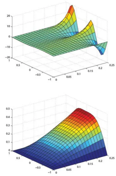
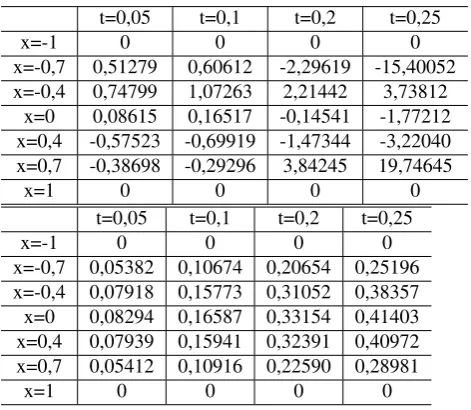
[image:5.595.67.292.426.598.2]

The below graphs and tables of calculations show that the values of approximate solutions with exact data and the values of approximate solutions with approximate data are nearly close to each other.

Figure 1.The Graph of approximate solution uN_{(x, t), v}N_{(x, t)}

[image:5.595.332.533.468.773.2]

for ac-curate data.

Figure 2.The Graph of approximate solution uNε(x, t), vNε (x, t)

[image:6.595.42.274.82.287.2]

Table 1.Approximate solution uN_{(x, t), v}N_{(x, t)}

for accurate data

t=0,05 t=0,1 t=0,2 t=0,25

x=-1 0 0 0 0

x=-0,7 0,51274 0,60606 -2,29596 -15,399 x=-0,4 0,74791 1,07252 2,21422 3,73774 x=0 0,08614 0,16516 -0,14539 -1,77194 x=0,4 -0,57518 -0,69912 -1,4733 -3,22008 x=0,7 -0,38694 -0,29293 3,84206 19,74447

x=1 0 0 0 0

t=0,05 t=0,1 t=0,2 t=0,25

x=-1 0 0 0 0

x=-0,7 0,05381 0,10673 0,20652 0,25194 x=-0,4 0,07917 0,15772 0,31049 0,38353 x=0 0,08293 0,16586 0,33151 0,41399 x=0,4 0,07938 0,15939 0,32387 0,40968 x=0,7 0,05412 0,10915 0,22588 0,28978

x=1 0 0 0 0

Table 2. Approximate solution uN

ε(x, t), vεN(x, t)

of the approximate data

t=0,05 t=0,1 t=0,2 t=0,25

x=-1 0 0 0 0

x=-0,7 0,51279 0,60612 -2,29619 -15,40052 x=-0,4 0,74799 1,07263 2,21442 3,73812

x=0 0,08615 0,16517 -0,14541 -1,77212 x=0,4 -0,57523 -0,69919 -1,47344 -3,22040 x=0,7 -0,38698 -0,29296 3,84245 19,74645

x=1 0 0 0 0

t=0,05 t=0,1 t=0,2 t=0,25

x=-1 0 0 0 0

x=-0,7 0,05382 0,10674 0,20654 0,25196 x=-0,4 0,07918 0,15773 0,31052 0,38357 x=0 0,08294 0,16587 0,33154 0,41403 x=0,4 0,07939 0,15941 0,32391 0,40972 x=0,7 0,05412 0,10916 0,22590 0,28981

x=1 0 0 0 0

5

Conclusions

Results of numerical experiments showed the effectiveness of the proposed approach.

Choosing parameter regularization from the optimality of estimate of the norm of difference between exact and approx-imate solution give for us possibility to stable calculation. We can see approximate calculation depends from the choosing of correctness set and parameter of regularization.

REFERENCES

[1] Igor S. Pulkin. Gevrey problem for parabolic equations with changing time direction. Electronic Journal of Differential Equations, Vol. 2006, No.50, pp. 1-9.

[2] Levine H.A. Logarithmic Convexity, First order Differential Inequalities and Some Applications. / Trance. of AMS, v.152, November 1970.

[3] Lavrentev, M.M. Conditional-correct problem for differential equations. Novosibirsk: NGU, 1973. 72 p. (In Russ.)

[4] Tersenov, S.A. Parabolic equations with a varying direction of time. Novosibirsk, 1985. 105 p. (In Russ.)

[5] Fayazov K.S. Ill-posed boundary value problem for a mixed-type equation of the second order. Uzbek Mathematical Jour-nal, 1995. No.2, p. 89-93

[image:6.595.42.278.321.526.2]