Journal of Chemical and Pharmaceutical Research, 2013, 5(12):623-630
Research Article
CODEN(USA) : JCPRC5
ISSN : 0975-7384
An ensemble based locality sensitive image clustering method
Haolin Gao, Bicheng Li, Yongwang Tang and Han Wei
Zhengzhou Information Science and Technology Institute, Zhengzhou, China
_____________________________________________________________________________________________
ABSTRACT
The main cluster algorithm in image clustering especially visual dictionary construction is still k-Means currently. The limitation of k-Means seriously deteriorates its feasibility for large image set, so we propose an Ensemble based Locality Sensitive Clustering method, which is based on distance and separability preservation property of random projection and the rationale of Exact Euclidean Locality Sensitive Hashing. It first determines the number of clusters of dataset, and then generates the multiple clustering resolutions, at last, applies cluster ensemble methods to get final partition. This method can make use of the advantage of Locality Sensitive Hashing, and improve clustering accuracy by cluster ensemble. The experiments showed that it achieved high cluster accuracy. In addition to its advantage of fast running speed, low cost and dynamic clustering, Ensemble based Locality Sensitive Clustering is a promising method for image cluster.
Key words: Exact Euclidean Locality Sensitive Hashing; random projection; image clustering; cluster ensemble _____________________________________________________________________________________________
INTRODUCTION
Though many clustering algorithms have been developed these years, most of them don’t work well in image clustering, especially in visual dictionary construction. The common used clustering algorithm is still k-Means, perhaps because it is difficult to design a general clustering to substitute k-Means. But the drawback of k-Means will become notable for large dataset especially ever-increasing dataset, because of its low running speed and high computation cost.
Random projection is a technique used in many areas such as reducing n-dimension points in Euclidean space to a random d-dimensional subspace, where d is much less than n. The Johnson-Lindenstrauss lemma implies that with high probability, relative distances and angles between all pairs of points are approximately preserved. This kind of random projection has a number of uses including fast approximate nearest-neighbor [1][2], clustering[3][4], signal processing[5], anomaly detection[6], dimension reduction[7][8] and so on. Moreover, random projections have also been applied to classification for a variety of purposes [9][10].
E2LSH(Exact Euclidean Locality Sensitive Hashing) is a special case of random projection, and it is first introduced as approximate near neighbor algorithm[11]. It has attracted much attention in recently, and was widely used in many areas such as image retrieval[12] and copy detection[13]. After projection, the data points saved in the same bucket are much similar than those in different buckets. So, if we divide a dataset according bucket indices into groups, the task of data clustering can also be achieved approximately. What’s more, E2LSH is a data independent method, which means the projection of a data point is independent of other points, so it can create a dynamic index for an incremental dataset. In fact, the introducer of LSH has pointed that LSH can serve as a fast clustering algorithm, but he didn’t testify it. E2LSH was applied for noun clustering by Ravichandran D[14]. However, Image data are more complicated than text word data, so clustering image is more difficult than clustering word data, but noun clustering can provide us with some useful information.
clustering ensemble, which makes use of the advantage of Locality Sensitive Hashing(LSH) and clustering ensemble. The merit of these two algorithms makes ELSC possible to be a promising clustering method.
RANDOM PROJECTION AND SEPARABILITY PRESERVATION
A random projection from n dimensions to d dimensions is represented by a n d matrix A. It does not depend on the data and can be chosen rapidly. The Johnson-Lindenstrauss Lemma shows that the distance of data points are preserved after projection. This makes it capable for approximate nearest neighbor search in information retrieval. Only distance preservation is not sufficient for clustering, the preservation of the class margin of data set is also necessary.
The Johnson-Lindenstrauss Lemma is famous for the distance preservation property. It can be described as: Given
0 1and any set S in n, for a positive integer
2 3
1
4( ) log
2 3
d S O(12logS)
, there exists a map
: n d
f , such that for all u v, S,
2 2 21 uv f u( )f v( ) (1 ) uv (1)
This lemma indicates that all pairwise distances are preserved up to 1 with high probability after mapping.
Let u v, n
, u 1 uA d
and v 1 vA d
where A is n d random matrix, whose entries are chosen
independently from either N(0,1) or U( 1,1) , then
( 2 3)2 2 2
4
Pr 1 (1 ) 1 2
d
A u v u v u v e
(2)
Imagine a set S of data in some high-dimensional space n
, and suppose that we randomly project the data down to
n
. By the Johnson-Lindenstrauss Lemma,
2
log
dO S is sufficient so that with high probability, all angles between points changed by at most / 2[15]. In particular, consider projecting all points in Sand the target vector
, if initially data was separable by margin , then after projection, since angles with have changed by at most / 2, the data is still separable.
Besides distance preservation, the margin preservation and angle preservation can be helpful in clustering. Shi et al established the conditions under which margins are preserved after random projection, and show that error free margins are preserved for both binary and multiclass problems if these conditions are met[16]. Balcan et al studied the problem of margin preservation under random projection for binary classification, and provided a lower bound on the number of dimensions required if a random projection was to have a given probability of maintaining half of the original margin[8], but it demands infinite many projections in order to guarantee the preservation of an error free margin. They provided two margin definitions below:
Normalized Margin: A dataset S is linearly separated by margin if there exists ud
, such that for all ( , )x y S,
,x y
x u
u (3)
Error-allowed Margin: A data distribution D is linearly separated by margin with error , if there exists
d
u , such that
( , )
, Pr
x y D
x y
x
u u
(4)
2
1 ln
c n
(5)
for an appropriate constant c, the projected data has margin / 2 with error and probability at least 1 . Equal (4) shows that a positive margin implies = 0, by which equal (5) implies that n . Thus, in order to preserve a positive margin in the projected data, infinitely many random projections are necessary.
As to angle preservation, any w x, d, any random Gaussian matrix Rn d, , for any (0,1), if w x, 0,
then with probability at least
2 3
1 6 exp
2 2 3
n
, the following holds
2
, w, x ,
1 2 1 1
1
1 1 w x 1 1 1
w x w x
w x w x
R R
R R (6)
E2LSH AND ENSEMBLE BASED LOCALITY SENSITIVE CLUSTERING
E2LSH is a special case of LSH, and it is also a random projection based method, this can be seen from the definition of hashing function. The k hashing functions are generated by random methods, and the inner-product perform the data projection. But it is different from general random projection. Each data point is projected by k
hashing functions, and the results are k bucket indices, which were representation of a point. The k hashing functions also indicate difference from general random projection in two ways. The first is the projection itself, the projection were not performed on the whole axis of some direction, but on parts of the axis. The second is that general projection is done by a matrix operation(a data point multiplies a n d random projection matrix A), but this is converted to a data points multiplies a single hashing function(a vector). It means the matrix operation is omitted in E2LSH algorithm. This is very important for large scale data processing, because matrix operation is nearly infeasible or high computation and memory cost.
Based on the former separability description, a dataset could be distance, margin and angle preservation after random projection. These properties make E2LSH feasible for data clustering. In fact, the points with same bucket index are more similar than those with different bucket index. So, if we group the data points with same bucket or adjacent buckets into a class, then the destination of data clustering is achieved approximately. Based on this, we propose Ensemble based Locality Sensitive Clustering(ELSC) to clustering images.
The original LSH hash function is designed for points in hamming space {0,1}d
. For Euclidean space, though it is possible to embed into hamming space, it increases the query time and error rate at a large extent and makes the algorithm more complicate. E2LSH can work directly in Euclidean space without embedding, it also works for any
(0, 2]
p for lp norm.
The single hashing function in E2LSH is defined as:
( ) a v b
h v
w
(7)
where a is a n-dimension vector generated by p-stable distribution function, and inner-product (a v ) work as a single channel random projection, b is the offset added to the random projection, and the module operation ensure the hash value(bucket index) is in a smaller range.
The hash function is similar to LSH, projected points in n
to k
:
1
{ : d k}, ( ) ( ( ), ( ))
k
g g v h v h v
(8)
The ELSC is based on E2LSH and cluster ensemble. The method mainly includes three parts, the number of clusters is determined in first part, the multiple locality sensitive clustering solutions are generated in second part, the clustering solutions are aggregated in third part.
Determining the number of clusters k of a dataset is important before clustering, which can be done by cluster validation analysis. The main goal of cluster validity analysis is to evaluate the results of a clustering algorithm. In general terms, there are three approaches to investigate cluster validity. The first is based on external criteria. This implies that the results of a clustering algorithm is evaluated based on a pre-specified structure, which is imposed on a data set. The second approach is based on internal criteria. The result of a clustering algorithm is evaluated in terms of quantities that involve the vectors of the data set themselves. The third approach is based on relative criteria by comparing one clustering solution to others.
The first approach need cluster labels of data point are provides, the relative approach is mainly used in cluster ensemble or to decide an optimal clustering method, so we use the second approach to estimate the cluster number. And the validity indices we adopt are Silhouette width(SI), Davies-Bouldin(DB) index and weighted inter to intra(Wint) similarity measure.
The silhouette of an object is a measure of how closely it is matched to others within its cluster and how loosely it is matched to objects of the neighboring cluster. A silhouette close to 1 implies the object is in an appropriate cluster, while a silhouette close to -1 implies the datum is in the wrong cluster.
For object i, the silhouette is defined as
( ) ( ) ( )
max{ ( ), ( )}
b i a i Sil i
a i b i
(9)
where a(i) is the average distance between i and all other objects in the same cluster, and b(i) is the average
distance between iand the objects in other cluster, i.e. ( ) 1 ( , )
i
j C i
a i d i j C
,\ ( )
( )
1 ( , )
( ) min
( ( )) ( )
k
C C C i
j C i k d i j b i
n C i n C
.The silhouette width is the average of each object's silhouette value, it lies in the interval [-1, 1], and should be maximized.
The DB index makes use of similarity measure Rij between the clusters Ci and Cj, which is defined upon a measure of dispersion (si) of a cluster Ci and a dissimilarity measure dij between two clusters. Rij is
formulated as i j ij ij s s R d (10)
where dij and si can be estimated by the following equations. Note that vx denotes the center of cluster Cx and
x
C is the number of objects in cluster Cx, dij d v v( ,i j),
1 ( , ) i i i x C i
s d x v
C
.Following that, the DB index is defined as
1 1 ( ) k i i DB R k
(11)where
1 ,
max
i ij
j k i j
R R
.
The DB index measures the average of similarity between each cluster and its most similar one. As the clusters have to be compact and separated, the lower DB index indicates better goodness of a data partition.
is to maximize intra-cluster similarity and minimize inter-cluster similarity, given by
,2
intra(X, , )= ( , )
1 a b i b a a b
i i
i s x x
n
and ,2
inter(X, , , )= ( , )
a b i b a a b
i j
i j s x x
n n
, where i and j are clusterindices. Note that intra-cluster similarity is undefined for singleton clusters. Then, the quality measure of Wint is based on the ratio of weighted average inter-cluster to weighted average intra-cluster similarity. The definition is:
1
1, ( )
1
inter(X, , , ) (X, ) 1
intra(X, , ) k
k i
j i
j j i
Q i
k i i
n
n i j n n n i
(12)( )
[0,1]
Q
, and ( )Q 0 indicates that objects within the same cluster are on average not more similar than objects from different clusters. On the contrary, ( )Q 1
indicates that every pair of objects from different clusters has the similarity of 0 and at least one sample pair from the same cluster has a non-zero similarity. To achieve a high quality ( )Q
as well as a low k, define a penalized quality (T )
. It is defined as:
(T ) 2 ( )
( ) (1 k) Q ( )
k k
n
(13)
For large n, the optimal k is searched in the entire window between 2 and n/ 2 or n 2. In many cases, however, a forward search starting at k=2 and stopping at the first down-tick of penalized quality while increasing k
is sufficient.
The final k is voted by these three indices. With the cluster number, the following the two parts can be continued. The overall procedure is showed as follows:
Step 1, determine optimal cluster number k by three validity indices SI, DB index and Wint for data set S.
Step 2, generate n k random matrix A(A A1, 2An)T from Gaussian distribution, and generate b, w according
the definition of LSH function, Ai is a k dimension vector, n S .
Step 3, perform random projection for all points viS, for each point vi, the results are k dimension bucket
indices Bi (B Bi1, i2Bik)
i i
v A b B
w
(14)
Then, for all points, the bucket indices are n k matrix B. Each column of B is a projection for whole dataset.
Step 4, clustering each column of B to k groups by PAM algorithm to get k partition, denoted as
1, 2,,k
. This step is different from LSC, because different projection results in different bucket indices, which means that the columns of B are different. So the quantification intervals of each column of B are also different, and it is difficult to choose property quantification intervals for each column. Therefore, we perform one dimension cluster for bucket indices for each column of B to get k partitions.Step 5, aggregate the k partitions by cluster ensemble method to get the final partition. The cluster ensemble methods include CSPA, HGPA and MCLA, and they attain three ensemble partitions, denoted as
1, 2 , 3
, thenthe final partition is one has max normalized mutual information with other two partitions among them,
2
* ( )
ˆ 1
ˆ arg max NMI ( , )
q q
EXPERIMENTS
We constructed an image set comes from TRECVID image set, containing four categories and 75 images total, parts of images are showed in Figure 1, the 4 categories includes ‘compere’, ‘singer’, ‘rice’ and ’sports’. The reason why we choose these images is that the inter-cluster different of them are notable distinct, and this is convent to verify the results of new clustering method.
[image:6.595.88.340.143.275.2] [image:6.595.95.521.392.444.2]
Figure 1 Parts of images in image set Figure 2 The clustering results of k-Means
[image:6.595.230.399.504.621.2]Because the ELSC is based on cluster ensemble method, we compare it with cluster ensemble based k-Means(Ek-Means). The cluster ensemble method in the Ek-Means is same as ELSC. We run Ek-Means and ELSC on the image set. To compare the performance, we first run k-Means on this image set. The results of k-Means on image set 1 are showed in figure 2. The multiple clustering resolutions of each point in the second cluster were showed in table 1.
Table 1 The clustering resolutions of k-Means for the 2nd cluster
Image index 1 2 3 4 5 6 7 8 9 10 11 12 13 14 15 16 17 18 19 20 Label 1(Correlation) 1 1 1 1 1 1 1 1 1 1 1 1 1 1 1 1 1 1 1 1 Label 2(CityBlock) 1 4 4 4 4 4 4 4 4 4 4 4 4 4 4 4 4 4 4 1 Label 3(Cosine) 4 4 4 4 4 4 4 4 4 4 4 4 4 4 4 4 4 4 4 4 Label 4(Euclidean) 1 2 2 2 2 2 2 2 2 2 2 2 2 2 2 2 2 2 2 1
Then we run cluster ensemble methods on these clustering solutions, the final cluster label is [1 1 1 1 1 1 1 1 1 1 1 1 1 1 1 2 2 2 2 2 2 2 2 2 2 2 2 2 2 2 2 2 2 2 2 3 3 3 3 3 3 3 3 3 3 3 3 3 3 3 3 3 3 3 3 4 4 4 4 4 4 4 4 4 4 4 4 4 4 4 4 4 4 4 4]. So, we can see that even there are some mistakes in clustering solutions, the final solution of Ek-Means is still totally correct according the original label.
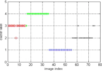
Figure 3 The final cluster label of ELSC
Table 2 The bucket indices of ELSC for the 2nd cluster
Image index 1 2 3 4 5 6 7 8 9 10 11 12 13 14 15 16 17 18 19 20 bucket indices 1 42 40 39 36 37 49 39 39 40 40 40 39 41 40 34 42 47 39 40 52 bucket indices 2 15 8 8 10 10 8 9 9 13 8 8 10 9 9 9 9 9 8 8 13 bucket indices 3 24 26 26 26 25 28 27 25 25 26 26 25 26 26 25 26 27 27 26 19 bucket indices 4 15 7 7 9 9 5 7 11 10 9 9 15 9 9 10 8 7 8 8 17 bucket indices 5 25 14 14 15 16 11 13 13 16 14 14 11 15 15 18 15 13 15 14 23
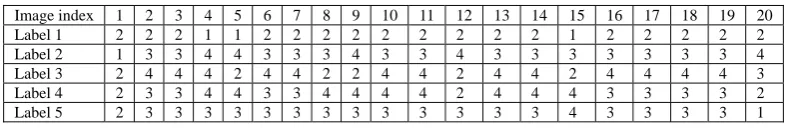
The multiple clustering solutions can be generated from these bucket indices by PAM clustering, and the results of step 4 in ELSC are showed in table 3. Only indices of the second cluster are given.
Table 3 The clustering solutions of ELSC for the 2nd cluster
Image index 1 2 3 4 5 6 7 8 9 10 11 12 13 14 15 16 17 18 19 20 Label 1 2 2 2 1 1 2 2 2 2 2 2 2 2 2 1 2 2 2 2 2 Label 2 1 3 3 4 4 3 3 3 4 3 3 4 3 3 3 3 3 3 3 4 Label 3 2 4 4 4 2 4 4 2 2 4 4 2 4 4 2 4 4 4 4 3 Label 4 2 3 3 4 4 3 3 4 4 4 4 2 4 4 4 3 3 3 3 2 Label 5 2 3 3 3 3 3 3 3 3 3 3 3 3 3 4 3 3 3 3 1
At last, we run three cluster ensemble methods for these clustering solutions, and select the best aggregated solution as the final partition. The final cluster label is [3 3 3 3 3 3 2 3 3 3 3 3 3 3 3 3 4 4 4 4 4 4 4 4 4 4 4 4 4 4 4 4 4 4 4 1 1 1 1 1 1 1 1 1 1 1 1 1 1 1 1 1 1 1 1 2 2 2 2 2 3 2 2 2 2 2 2 2 2 2 2 2 2 3 3], the clustering accuracy is 93%.
Though it is still slightly less than k-Means. But the advantage of ELSC is dynamic clustering, fast clustering, low memory cost and low computation cost. The former two merits are decided by the property of itself, and the latter two merits have been verified in related literatures. So, ELSC is a promising clustering method in high dimensional space.
CONCLUSION
The Ensemble based Locality Sensitive Clustering method we proposed in this paper is the combination of cluster ensemble and Exact Euclidean Locality Sensitive Hashing, it possesses the advantage of E2LSH and discard the drawback of E2LSH. Its clustering accuracy achieves 93% in our experiments, though it is slightly less than Ek-Means for image set, but its advantage of dynamic fast clustering, low memory and computation cost. These make it a promising clustering method for large incremental high dimensional data set, because k-Means is nearly the only clustering method in image visual dictionary generation till now, and it has some limitations in bag of words method. The Ensemble based Locality Sensitive Clustering method could be a substitute for k-Means clustering in visual dictionary generation, and this will bring about the performance improvement of bag of words method in image classification, image recognition, image retrieval and other related areas.
REFERENCES
[1]Indyk P, Motwani R. Approximate nearest neighbors: towards removing the curse of dimensionality. In: Proceedings of the Symposium on Theory of Computing. Dallas, Texas, USA:ACM, 1998: 604-613.
[2]Sanjoy Dasgupta, Kaushik Sinha. Randomized partition trees for exact nearest neighbor search JMLR: Workshop and Conference Proceedings vol 30 2013:1-21
[3]Schulman, L. J. Clustering for edge-cost minimization. In Proc. Annual ACM Symp. Theory of Computing, 2000: 547-55.
[4]Tomoya Sakai and Atsushi Imiya. Fast Spectral Clustering with Random Projection and Sampling. Proceeding of The 9th International Conference on Machine Learning and Data Mining. 2009:372-384.
[5]Donoho, D. L. Compressed sensing. IEEE Trans. Information Theory, 2006.52(4):1289-1306. [6]James E. Fowler, Qian Du. IEEE Transaction on Image Processing2012 (21).1:184-195.
[7]Christos Boutsidis, Anastasios Zouzias, Petros Drineas. Random Projections for k-means Clustering. In Proceedings of Neural Information Processing Systems. 2010:298-306..
[8]Alon Schclara, Lior Rokachb, Amir Amit. Machine Learning, 65(1):79-94, 2006.
Conf. Image Processing, 2007. 6: 161-164.
[10]Shi, Q., Petterson, J., Dror, G., Langford, J., Smola, A. J., and Vishwanathan, S.V.N. J. Mach. Learn. Res.
2009.10:2615-2637.
[11]Andoni and P. Indyk. Communications of the ACM, 2008.51(1):117-122..
[12]Jegou H, Douze M, Schmid C. International Journal of Computer Vision, 2010, 87(3):316-336
[13]Liu Zhu, Liu Tao, David G. Effective and scalable video copy detection. In: Proceedings of the ACM SIGMM International Conference on Multimedia Information Retrieval. New York, USA:ACM, 2010: 119-128
[14]Ravichandran D, Pantel P, Hovy E. Randomized Algorithms and NLP: Using Locality Sensitive Hash Function for High Speed Noun Clustering. In: Proceedings of the 43rd Annual Meeting on Association for Computational Linguistics, Stroudsburg, PA, USA:ACM, 2005: 622-629.
[15]Avrim Blum. Random Projection, Margins, Kernels, and Feature-Selection. LNCS 3940, 2006:52-68.