MRI BRAIN SEGMENTATION VIA HYBRID FIREFLY
SEARCH ALGORITHM
1
WALEED ALOMOUSH, 2SITI NORUL HUDA SHEIKH ABDULLAH, 3SHAHNORBANUN SAHRAN, 4RIZUANA IQBAL HUSSAIN
123
Pattern Recognition Research Group, Center for Artificial Intelligence Technology ,Faculty of Information Science and Technology,Universiti Kebangsaan Malaysia, 43600, Bangi, Selangor D.E.,
Malaysia.
Department of Radiology Universiti Kebangsaan Malaysia Medical Centre, 56000 Cheras, Kuala Lumpur, Malaysia.
Email: [email protected] , [email protected] , [email protected] ,
ABSTRACT
Magnetic resonance imaging (MRI) brain tumor segmentation is a challenging tasks which include the detection task of tumor from images. In general, this process is done manually by experts in medical images field which is always unclear, because the similarity between normal and abnormal tissues. The present study proposes a new clustering approach based on the hybridization of firefly algorithm (FA) and fuzzy c-means algorithm(FCM) called (FFCM) to segment MRI brain images. this approach use the capability of firefly search to find optimal initial cluster centres for the FCM and thus improve (MRI) brain tumor segmentation. The proposed approach was evaluated by applying it to a magnetic resonance imaging (MRI) brain segmentation problem using a simulated brain data set of McGill University and real MRI images from Internet Brain Segmentation Repository benchmark data sets. The cluster validity index(Rm) was used as a fitness function to determine the best solutions obtained by the firefly algorithm. The experiments indicated encouraging results after applying FFCM, compared with the outcomes of state-of-the-art segmentation algorithms and FCM random initialization of cluster centres.
Keywords:Fuzzy c-means, Firefly algorithm, MRI Images segmentation, Rm validity index
1. INTRODUCTION
The process of digital image analysis comprises a lot of steps or phases, and image segmentation is one of the most significant and intricate. In this phase, images are segmented into many components and each component contains some identical attributes [1] . Image segmentation considered a basic role in many different domains. In medical imaging for instance, Magnetic resonance imaging (MRI) images segmentation techniques can assist doctors and radiologists locate tumors and other pathologies, diagnose illnesses, therapy evaluation, aid in computer guided surgery, measure tissue volume, treatment planning, study anatomical structure, and also surgical simulation [2]. Moreover, different sequences of MRI images are available from these imaging modalities such as T1-Weighted Image (T1WI), Short Tau Inversion Recovery (STIR), T2-Weighted Image (T2WI), Fluid Attenuation Inversion Recovery
ISSN: 1992-8645 www.jatit.org E-ISSN: 1817-3195
segmentation[5-6]. Both image segmentation and clustering share the same goal of finding accurate classification of their input. The image pixels in clustering methods represented as patterns and each pixel is belong to a cluster (image segment) based on similarity and distance[7].
Over the last few decades, many algorithms for metaheuristic search have been applied in conjunction with the FCM algorithm to find optimal cluster centres. These algorithms explore the entire search space in the problem to determine possible solutions[8]. These algorithms include bee optimization[9], harmony search[10], the ant colony algorithm[11], simulated annealing[12], the genetic algorithm[13-14], tabu search[15], the firefly algorithm[16] and particle swarm[17]. However, to the best of the authors’ knowledge, this present study is the first time that a firefly fuzzy c-means (FFCM) algorithm has been applied to image segmentation. Specifically, the present study explores the addition of a firefly algorithm (FA) to FCM to solve the brain MRI image segmentation problem because this is a very complicated domain due to the natural difficulties inherent in MRI image segmentation. The present study explores the efficiency of the FA in generating near-optimal initial cluster
centres for the FCM algorithm, in order to ensure that superior and constant MRI image segmentation outcomes are generated. The FA is one of the more recent algorithms, and as the name implies, is inspired by the behaviour of fireflies[18]. It is worth mentioning that the FA has been employed to resolve nonlinear optimization problems. Generally, in social insect colonies, such as a firefly colony, even though every single individual appears to have an individual routine, the group as a whole seems to be extremely structured. Basically, algorithms that are based on nature have been proved to be effective and efficient in resolving challenging optimization problems. A swarm is a collection of multi-agent systems, such as fireflies, in which the basic agents synchronize their routines to resolve the complicated issue of assigning communication to numerous forage sites in changing circumstances. The remainder of the paper is structured as follows: section 2 provides an overview of the firefly search algorithm; section 3 describes fuzzy clustering with FCM; section 4 discusses the proposed method; section 5 details the results of experiments applying the FFCM algorithm and compares them with other methods; and finally, section 6 presents the conclusion.
2. FIREFLY SEARCH ALGORITHM
Fireflies are among the rarest insects on the planet and have a natural capacity to illuminate themselves in the dark with flickering and glowing biological lights. The FA was motivated by the biological behaviour of fireflies[18]; generally, the FA employs the following three rules: (1) fireflies are unisexual, therefore every individual firefly will be fascinated by another firefly, irrespective of its gender; (2) the unique feature of the glowing light of fireflies will attract prey; and (3) the attraction of fireflies is proportionate to their brightness, which makes the less bright firefly move towards a more brightly glowing firefly .
The population-based FA is capable of discovering the global optima of objective functions, depending on the intelligence of the swarm[19]. Moreover, the FA also examines the foraging behaviour of fireflies. In the FA, the physical entities are arbitrarily spread in the search space, in this case the physical gentility is fireflies, which have a substance known as luciferin that makes the fireflies glow in dark, and generally luciferin will discharge light that is
proportional to this value. As mentioned earlier, the fireflies with slightly dimmer light will be attracted towards the brighter individuals; nevertheless the degree of attraction will reduce if the distance between those fireflies increases. On the other hand, if any firefly fails to find another firefly that is brighter than itself, then the former will travel arbitrarily. When the FA is employed to solve clustering problems, the cluster centres are the decision variables, and the objective function is associated with the value of all Euclidean distance training set cases in an N-dimensional space[20].
(fireflies), where x signifies the solution of a firefly i, while its fitness value is signified by
fx; furthermore, the current position i of its fitness value fx is determined by the brightness
I of a firefly[21], thus:
I fx, 1 i n . (1) The second stage involves movements towards attractive fireflies: the attractive force of a firefly is proportionate to the intensity of light witnessed by nearby fireflies[21]. Every single firefly possesses its unique attraction β, which indicates the power of attraction over individuals of the swarm. This attractiveness β will change with the distance r between two fireflies i and j at locations x and x, respectively, as denoted by the following:
r x x , (2) The attractiveness function β(r) of the firefly is established by
βr βeమ , (3)
if β is the attractiveness at r 0, and γ is the coefficient of the ingestion of light. The motion of a firefly i from position x, which is attracted to another much more attractive (brighter) firefly
j at position x is denoted by
Fig. 1. Firefly Algorithm Pseudo-Code.
x x βeౠమ x x ∝ rand
(4)
A comprehensive explanation of the FA can be found in[18] and the pseudo-code for this algorithm is given in Fig. 1.
3. CLUSTERING WITH FUZZY C-MEANS
Clustering is a unsupervised learning approach that is capable of partitioning identical data objects (patterns) based on some level of similarity, which increases the similarity of objects within a group and decreases the similarity among objects between various groups[22-23]. A clustering algorithm for grouping fuzzy data is carried out on a collection of n objects (pixels) x, x , … , x , and each of these objects is x ∈ ", a characteristic vector
which consists of d real-valued dimensions that reveal the characteristics of the object depicted by x . A fuzzy membership matrix, referred to as fuzzy partition U $u & (U ∈ M as in Eq. 1). The equation
MU ϵ
U 1, 0 U n
, an d U ∈ 0,1; 1 j c ,; 1 i n
5
represents the fuzzy clusters c of the objects, where signifies the fuzzy membership of the ith object to the jth fuzzy cluster. For example, each and every data object is related to a specific (probably zero) degree of every single fuzzy cluster. A FCM algorithm is a repetitive technique capable of locally decreasing the following objective functions:
J * * u
x
v , 6
where -v.
is the centroids of the clusters c,
which indicates the standard of the inner product
‖. ‖ (e.g., Euclidean distance) from the data point
x to the jth cluster centre; furthermore, the parameter m ∈ $1, ∞ is a distort proponent on each fuzzy membership, which ascertains the level of fuzziness of the ensuing classification. The following is a summary of the FCM steps and Fig. 2 below illustrates the FCM pseudo-code:
ISSN: 1992-8645 www.jatit.org E-ISSN: 1817-3195
3. Estimate the components of the fuzzy partition matrix:
U 1
∑ 3‖xx v‖4 v
7
4. Calculate the cluster centres:
v ∑ u . x
∑ u
8
5. Repeat steps 3 and 4 until the number of iterations (t) surpasses the set limit, or a termination criterion is met:
‖v v‖ 7 ε 9
where ε 7 0.001
Fig.2.FCM Pseudo-Code.
1. Proposed method
In this section we investigate the performance of the FA in terms of obtaining near-optimal cluster centres values in the initialization phase in the FCM algorithm. Here, we propose a clustering approach that consists of two phases (see Fig. 3 below). In the first phase, the FA examines the search space of the given data set to determine the near-optimal cluster centres and then those cluster centres are assessed by making use of the redefined FCM objective function. In the second phase, the finest cluster centres that have been identified are employed as the preliminary cluster centres for the FCM algorithm. The two phases are discussed below.
1.1 Identifying near-optimal cluster centres using firefly search
The cluster centres of the provided data set are encoded by each and every solution of the firefly search. The solution will be as in Eq. 10:
a
3aa … . a , aas s s … . a , aa … . a4 , 10
where a is a numerical characteristic that explains a cluster centre and a∈ A , where A is the collection of the feasible array of each and every pixel attribute. Consequently, each cluster centre s is defined by d numerical featurea, a , … , a . As a result, every single solution has an actual size of c < d, where c represents a given number of clusters and d indicates the feature number outlining the given data set.
Fig .3. Proposed FFCM Framework.
For the purpose of delineating the connection between the clustering and image segmentation, we claim that it is possible to map every single pixel in an image as a sample or data point in the clustering sector, while it is also possible to map the image regions as clusters or classes. In the case of a 256 x 256 image, there will be 65,536 pixels (data points). For instance, in a given grey image with three distinct regions (e.g., the white matter (WM), grey matter (GM) and
cerebrospinal fluid (CSF) in a MRI image of the brain), 8-bit depth, and three features (e.g., intensity value, entropy, and energy), which illustrate each and every pixel, the probable degree of pixel intensity value pertaining to the depth of image will be in the interval ∈[0,255], and the deterioration and energy features can be illustrated by interval ∈ $0, 10&. Therefore, the firefly solution could be (5, 2.5, 2.6, 30, 6.2, 2.1, 80, 2.3, 1.3), in which the first three digits (5, 2.5, 2.6) signify the cluster centre values for the first image region in each image sequence, and the next three digits (30, 6.2, 2.1) indicate the cluster centre values for the second image region, while the final cluster centre (80, 2.3, 1.3) indicates the third image spot. Immediately after the firefly sets the factors ((n) number of fireflies, β, γ, max generation), the initialization step of the firefly search is examined. All the cluster centres in all the solutions might be randomly initialized from the data range of their image attributes.
Then the fitness value is measured for all the solutions by the objective function and later, the solutions are reorganized in descending order of the objective function value. After choosing the minimal values by comparing the solutions with the objective function, the FA finds near-optimal cluster centres that guarantee that fuzzy c-means will reach near-global optima and will not be trapped in a local optima. This leads to an improvement on the FCM and thus FFCM can replace the traditional method of multiple random initializations to determine cluster centres.
ISSN: 1992-8645 www.jatit.org E-ISSN: 1817-3195
R * >* D
@
, 11
where D is x v the distance from pixel intensity x to the jth cluster centre, m is the fuzziness of the resulting classification and it is set m 2 and n is the total number of pixels in the given image. In this case, we measured the aggregate of the distances between all the pixels in the given image with each cluster centre that was produced from the new solution. However, the FA will attempt to reduce this value of R (cluster validity) to find the preferred near-optimal solution or to fulfil the stopping criterion.
The objective function is computed for each new firefly solution fa,for the purpose of updating the solutions with the newly generated, a a, a, a , … , a , if the value of objective function of the new solution is superior to theworst solution stored, then the latter is replaced by the new solution or else this new solution is disregarded.
The iteration process of the evolving procedures of the FA will be ended after achieving the optimum number of improvisations (max generations). Ultimately, the ideal solution is chosen and is regarded as the finest solution to the examined problem. However, such clustering methods consume a huge amount of time, especially in the case of a large number of objects [25].Therefore, it is essential to include a simplification phase to enhance the efficiency of the firefly search by minimizing the number of objects to be clustered, which in turn will minimize the time needed to find the near-optimal solution. The simplification process depends on obtaining the rate of incidence of each pixel in the examined image (like a histogram). Consequently, the image is depicted
in a model such as B C , D, … ,
C , D, … , C , D, where D is the rate of incidence C in the image and E is the total number of distinct C values in the image with
∑ D
F ). Therefore, the objective unction
can be reformulated as follows:
G
* D>* H!
"
!
@ 12 #
FCM-based clustering
The FCM algorithm starts with the cluster centers obtained from the FA as initial cluster centers at every iteration and it determines the fuzzy membership of each data point in relation to every cluster by Eq. 7. Based on the membership values, the cluster centers are recomputed by Eq. 8. The FCM stops when there is no further change in the cluster centers.
4. EXPERIMENTS AND RESULTS
This section explains the evaluation of the proposed solution (FFCM) and compares the outcomes with those of several previous methods and the results acquired from the conventional FCM clustering algorithm, namely the random initialization technique of FCM. This section is divided into six parts. The first part describes the data set. The second part analyses the FFCM parameters and the best parameter values are selected. In the third part, the cluster validity (Rm) index is introduced as a quality measurement. In the fourth part, the FFCM is applied to a simulated brain MRIdata set. In the fifth part, the FFCM is applied to a real brain MRI data set. In the final part, the execution times of FFCM for both types of image representation are presented.
4.1 Data set
The data set comprises two different groups of 3D MRI images for the purpose of illustrating the efficacy of the proposed FFCM algorithm. The first group comprises seven normal images and ten abnormal simulated T1-weighted MRI brain images (T1WI), which were acquired from the simulated brain data set of McGill University [26].The size of all these images is 217 × 181 with 8-bit greyscale level. The second group comprises 20 normal 3D MRI real images which were acquired from Internet Brain Segmentation Repository (IBSR), Centre for Morphometric Analysis, Massachusetts General Hospital Repository [27].
4.2 Analysis of firefly parameters
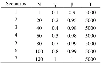
for various configurations to demonstrate the convergence behaviour of the FA. Every single designed case was executed 10 times with the repetition numbers set to 1,000 for all runs. We roughly tested different values for n varying from 1 to 120 and thereby identified that the acceptable value of n is close to 120. Consequently, the n in the majority of the examined cases (see Table 1) was fixed to 120, and every individual case was examined on three MRI real images and six MRI simulated images.
Table 1. Ffcm Convergence Scenarios.
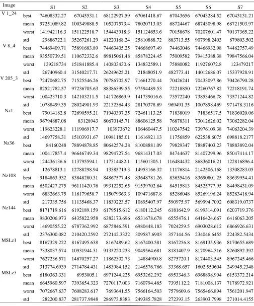
Table 2 illustrates the best, mean, worst, and standard deviation of the objective function of every single case. We have highlighted the ideal outcome in bold (i.e., minimum objective function as in Eq. 12) among all cases for every single image. Case S1 (scenario 1, Table 1; S1, Table 2) functions as a local search-based algorithm, which depends on one particular option, s. This case depends on the preliminary arbitrary solution. This inhibits the FA in terms of its ability to examine the search space of the presented image, because α=0.1. Moreover, it is not possible to enhance the solution. This case has weak effectiveness (see Table 2), because it quickly ends in local optima.
Case S2 shows the potential of the FA to boost a novel population of solutions that is dependent on the n of fireflies. This case exhibits the optimistic impact of a greater number of solutions. Case S2 outcomes are completely influenced by preliminary solutions, which are arbitrarily produced and saved. Nevertheless, the efficiency of the second case is superior to that of the first case, despite the fact that identical factors were used for these cases, besides the firefly search. However, they are both significantly less effective than cases S3 and S4 in which the exploration behaviour of the firefly
search is enhanced, because the light absorption coefficient is increased to β=0.98, and the potential of exploring unvisited regions of the search space is higher. Consequently, the convergence speed of the firefly γ reached γ=0.5 may be positively affected. In cases S5, S6 and S7, the firefly search utilizes the strength of the light absorption coefficient to pick superior solutions at this point. Similarly, the firefly search is capable of exploring unvisited regions in the given search space through using the light absorption coefficient, where β is 0.99 and 1 correspondingly. These cases are capable of utilizing the advantages of the firefly
search to simultaneously check several search space regions while focusing on the most encouraging regions, which consequently results in the most ideal outcomes being achieved by these cases. Based on our analysis, case S7 was chosen to carry out tests in this section, where the firefly variables are set as follows: n=120,
β=1, g=1 and the maximum number of iterations (t) is 5,000.
Scenarios N γ β T
1 1 0.1 0.9 5000
2 20 0.2 0.95 5000
3 40 0.4 0.98 5000
4 60 0.5 0.98 5000
5 80 0.7 0.99 5000
6 100 0.8 0.99 5000
ISSN: 1992-8645 www.jatit.org E-ISSN: 1817-3195
Table 2. Evaluation Of Ffcm Parameters
Image S1 S2 S3 S4 S5 S6 S7
V 1_24 best 74608332.27 67045531.1 68122927.59 67061418.67 67043656 67043284.52 67043131.21
mean 97251089.82 100349888.5 105207573.4 78020713.03 68724467 68743098.98 68721503.97
worst 141942116.3 151122518.7 154443918.3 151124653.6 70158678 70207601.47 70137365.22
std 29886722.1 35267261.29 41220168.24 25810888.72 883713.55 907998.2403 879803.502 V 8_4 best 74469409.71 75891683.89 74463405.25 74668697.49 74463046 74466932.98 74462757.49
mean 93550739.51 110672332.6 89815061.48 85878224.45 75009582 79415388.38 79847566.04
worst 139218734 151841885.4 140803430.6 134832589.1 75880082 119276072.8 123479217
std 26740960.4 31540217.71 26249625.21 21848051.9 482773.41 14012686.07 15337928.91 V 205_3 best 72470682.75 71525546.26 70786702.97 71661270.44 70426241 70433097.86 70426790.28
mean 82521782.57 97236705.63 88386399.55 97594489.53 72218850 72260767.82 72218191.74
worst 100423710.3 142103211.5 141726869.9 141739016.6 73572240 73853466.78 73571244.82
std 10788499.35 28024901.93 22132364.43 28170378.69 969491.35 1007898.469 971478.3116 Nz1 best 79014182.8 72690595.21 71940397.35 72461113.25 71838019 71836517.5 71836020.06
mean 96794887.08 83128943 80670145.71 88606125.58 76878311 73012626.02 73062282.04
worst 119623228.1 111906917.7 103973672 106460447.5 110247542 73976109.38 74063204.39
std 14697758.31 15103931.67 10981185.01 11616921.13 11756859 622538.6075 698818.2177 Nz36 best 84160248 78894878.85 80642574.28 81008881.09 79829347 78887403.23 78883892.04
mean 100417857.4 96646749.34 98294727.54 96814317.03 84744637 81407299.96 85047414.17
worst 124436136.6 113795594.1 117314482.1 115601305.1 116484432 86836016.21 122816896.4
std 12678813.1 12788298.94 13385719.3 14953166.32 11176814 2142506.168 13308283.05 Nz108 best 9184863.932 83848280.31 84867577.48 83648781.26 83655416 83690801.25 83639954.41
mean 6502427.275 96111420.76 99312252.65 91539702.64 84515813 84525777.95 84498431.09
worst 6832663.75 116179658.7 115079363.3 109471687.8 85286048 85269196.24 85283418.94
std 217335.756 11135468.37 11839223.57 10895407.97 590975.97 569994.7092 608319.0737 Nz144 best 8171719.616 6192189.159 6179515.612 6180112.245 6181642.9 6199314.091 6203719.376
mean 9830206.973 6435822.958 6382173.696 6531678.678 6555476.1 6416424.667 6416063.205
worst 14690555.22 6787362.992 6875846.591 6980448.183 7024259.5 6903028.612 6866926.631
std 2376300.082 210420.2592 272142.3322 309587.6903 357144.56 234046.6455 224382.5434 MSLz1 best 8167329.222 8167495.638 8167489.62 8167400.581 8167256.8 8169135.936 8170655.689
mean 7338037.574 10931944.31 9135220.233 9049564.681 8181407.9 8170964.316 8260892.392
worst 7627236.571 14670257.27 11862302.73 14884900.8 8275720.1 8174403.545 8967245.466
std 313774.6939 2714784.431 1483984.152 2146576.766 33368.657 1602.550604 249945.2348 MSLz5 best 6180363.331 6953005.1 6971244.225 6953262.292 6953346.3 6968898.994 6153372.214
mean 6645960.597 7393654.323 7270117.003 7160794.485 7395112.2 7181008.137 7178972.921
worst 7072667.637 7608283.617 7693641.55 7566164.503 7579609.6 7565466.894 7561201.947
Table 3. Comparative Results (Rm) Between Fcm And Fcm.
Table 4. Comparative Results Based On Different Validity Indices And Objective Function.
Image Method PC PE XB Rm
V 1_24 FFCM 0.879404 0.237179 0.000799 67043749
FCM 0.879405 0.237178 0.000799 67430684
V 8_4 FFCM 0.865383 0.264834 0.000803 74696567
FCM 0.865384 0.264831 0.000803 75974061
V205_3 FFCM 0.867526 0.261788 0.000895 70428267
FCM 0.867529 0.261783 0.000895 70795134
Nz1 FFCM 0.864492 0.267963 0.00087 71892044
FCM 0.864511 0.267928 0.00087 87755933
Nz36 FFCM 0.846116 0.302557 0.001052 78888625
FCM 0.846146 0.3025 0.001052 84434510
Nz108 FFCM 0.84053 0.31214 0.001 83643996
FCM 0.84055 0.312103 0.001 85667812
Nz144 FFCM 0.778607 0.183036 0.001471 6241319
FCM 0.777622 0.183663 0.101295 6533914
MSLz1 FFCM 0.897963 0.089005 0.000506 8167285
FCM 0.89797 0.088998 0.036825 12918686
MSLz5 FFCM 0.862987 0.114635 0.000846 7025565
FCM 0.841994 0.130859 0.10682 7093692
images FFCM FCM
AVG Rm SD± AVG Rm SD±
V 1_24
68730248 885809.1 74313563 11301955
V 8_4 74998354 478511.8 85187983 11770134
V 205_3 79030282 21794694 79319368 8836978
Nz1 72996452 619726.8 92058746 25458388
Nz36
83929453 9330378 84778061 5342354
Nz108 87270510 8808884 87843696 3891235
Nz144 6424714 265892 7074611 629600.4
MSLz1 4372070 97024 7030067 8786194
MSLz5
ISSN: 1992-8645 www.jatit.org E-ISSN: 1817-3195
5.3 Cluster validity index
The excellence of the solution created is assessed with regards to the intent function. The tests are designed to analyse the efficiency of the firefly search in obtaining suitable preliminary cluster centres for the FCM algorithm, as against the conventional random initialization technique employed to select cluster centres. The outcomes for the FCM with firefly search initialization are designated as FFCM, whereas the outcomes for the FCM with random initialization are denoted as FCM. In the present study we employed the intent function value as a measure of the goodness of clustering. We documented the typical and the standard deviation results of FCM and FFCM from 50 trials. All the tests were carried out on an Intel Core5Duo 2.5 GHz machine, with 4GB RAM. The codes were written using Matlab 2010a.
Table 3 illustrates the above mentioned outcomes, where the first column represent images name, the second column signifies the average and standard deviation value for objective function acquired from the search process of the FA in identifying near-optimum cluster centres, and the initial stage of FFCM method. The third columns depict the average objective function and standard deviation value for FCM, respectively.
These outcomes indicate that the majority of the analysed images show considerable enhancements with respect to minimization of objective function values when using the proposed algorithm FFCM as against FCM. The bold items in Table 3 signify equivalent or superior outcomes of FFCM as compared with FCM. In addition, and from a more detailed investigation of these results , it is evident that FFCM is more constant and reliable than FCM with respect to the acquired standard deviation measurements. On the ther hand, some images still failed to display any enhancements. This result encouraged the author to employ another better measurement and examine the effectiveness of using the objective function as a measurement of the superiority of clustering outcomes. Hence, a cluster quality listing was employed as a functionality metric. A cluster quality list is generally applied to gauge the quality of clustering algorithms.
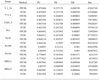
The present study employed three of the most well-known fuzzy cluster validity indices, namely the PC, PE, XB, in addition to the Rm. These indices are primarily employed to gauge the solidity and uniqueness of the clustering
results. A decrease in the values of the XB and PE indices is preferred, whereas an increase in the PC index value is viewed as ideal. Hence a reduction or an improvement in these indices discloses the quality of the clustering. The values in Table 4 illustrate the outcomes with respect to utilizing these cluster validity indices as quality measurements. The result of FCM and FFCM applied to each image is shown for each index. To aid our analysis of the results presented in Table 4, we categorized the images into two groups. The first group of outcomes closely estimated the objective function values between FFCM and FFCM, as in cases 1, 3 and 9. The second group has lower objective function values for FFCM as against FCM, as in cases 2, 4, 5, 6, 7 and 8. The first group is a normal case, where the estimated values of the objective function obtained by FFCM and FCM need to suggest estimate values for the outcomes acquired by cluster validity indices, which is the case that has been obtained. In the second group, the values of the objective function obtained by FFCM are significantly lower than those of FCM. This is superior regarding the objective function, which has been employed and the outcomes acquired by cluster validity indices reveal in the identical course, where the values of cluster validity in FFCM is superior than FCM, which is also the case, which has been acquired. This means that based on the objective function values, the clustering output of FFCM is better than that of FCM. Consequently, the outcomes acquired from our proposed algorithm are superior to those of the FCM algorithm with random initialization across the four quality measurements used here.
5.4 Simulated MRI brain data
regions’ tissues have the same intensity in the MRI images such as the WM and connective tissues, skull and background, skin and CSF. Therefore, in the present study after merging those regions having the same level of intensity and removing the skull, the clusters numbered six in the normal images and seven in the abnormal images.
The Brain Web [26] provided the ground truth images, and a quantization index was used to evaluate segmentation performance, based on the segmentation accuracy. The accuracy rate was
computed based on the similarity between the ground truth image and the segmented images generated by FFCM and FCM. The Minkowski Score (MS) is the quantization index used in the present study [28], which is computed as follows:
IJK, J L#బభ#భబ
[image:11.612.91.532.186.339.2]#భభ#భబ , 13
[image:11.612.94.531.393.502.2]Fig. 4a. From Left To Right, Original Normal MRI T1 Image In Z1, Ground Truth Normal MRI T1 Image In Z1, And Normal MRI T1 Image In Z1 Segmented By FFCM.
Fig. 4b. From Left To Right, Original Normal MRI T1 Image In Z36, Ground Truth Normal MRI T1 Image In Z36, And Normal MRI T1 Image In Z36 Segmented By FFCM.
[image:11.612.90.525.544.656.2]ISSN: 1992-8645 www.jatit.org E-ISSN: 1817-3195
[image:12.612.90.559.380.495.2]
Fig. 5a. from left to right, original multiple sclerosis lesions in MRI T1 image in z1, ground truth multiple sclerosis lesions in MRI T1 image in z1, and multiple sclerosis lesions MRI T1 image in z1 segmented by FFCM.
Fig 5b. from left to right, original multiple sclerosis lesions in MRI T1 image in z5, ground truth multiple sclerosis lesions in MRI T1 image in z5, and multiple sclerosis lesions in MRI T1 image in z5 segmented by FFCM.
[image:12.612.119.493.553.699.2]
Fig. 5c. from left to right, original multiple sclerosis lesions in MRI T1 image in z10, ground truth multiple sclerosis lesions in MRI T1 image in z10, and multiple sclerosis lesions in MRI T1 image in z10 segmented by FFCM.
TABLE 6. Comparative results: Minkowski Score (MS) for abnormal brain images showing multiple sclerosis lesions.
Z plane MS (FFCM) MS (FCM) MS(EM)
1 0.39 0.64 1.21
2 0.38 0.64 0.80
3 0.78 0.76 0.74
4 0.33 0.73 0.79
5 0.32 0.65 0.69
6 0.32 0.78 0.85
7 0.35 0.76 0.74
8 0.36 0.78 0.79
9 0.38 0.73 0.76
where T represents the ground truth image and S represents the segmented image. F represents the number of pairs of elements that are in the same region in both T and S, while F represents the number of pairs in the same region in T and F represents the number of pairs in the same region only in S. The best similarity between the ground truth image (T) and the segmented image (S) is the minimum value of the MS, where the best value for MS equals 0. In the first experiment (normal simulated MRI brain images), the MS accuracy rate obtained by FFCM showed very good segmentation outcomes. Table 5 shows that the MS accuracy rate obtained by FFCM was much better than that by FCM for five segmented images (z1, z2, z3, z36, z108) and MS accuracy rate obtained by FFCM was much better than that by Expectation Maximization (EM) for five segmented images (z1, z2, z3, z36, z144). While The MS for FCM is better than FFCM for two segmented images (z72, z144) and the MS for EM is better than FFCM for two segmented images (z72, z108) because the ground truth images have a different number of clusters, and thus the matching MS test was affected. Figure 4 shows, from left to right respectively, the original image, ground truth image and image segmented by FFCM. In the second experiment (abnormal simulated MRI brain images), the MS accuracy rate obtained by FFCM produced excellent segmentation outcomes. Table 6 shows that the MS accuracy rate obtained by FFCM was much better than that by FCM and EM for nine segmented images (z1, z2, z4, z5, z6, z7, z8, z9, z10), while the rest were comparable. The MS for FCM and EM was better than for FFCM for one segmented image (z3) because the ground truth images have a different number of clusters, and thus the matching test (the MS) was affected. Figure 5 shows, from left to right respectively, the original image, ground truth image and image segmented by FFCM.
TABLE 5: Comparative Results: Minkowski Score (MS) For Normal Simulated Images.
Z plane MS (FFCM) MS (FCM) MS(EM)
1 0.39 0.7 1.019
2 0.38 0.65 0.83
3 0.36 0.62 0.64
36 0.87 0.88 1.12
72 0.78 0.72 0.70
108 0.61 0.79 0.58
144 0.69 0.34 0.76
5.5 Real MRI brain data
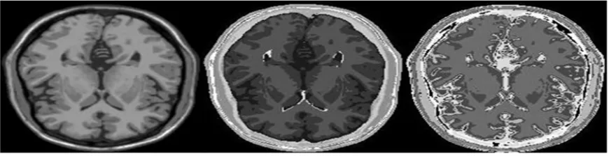
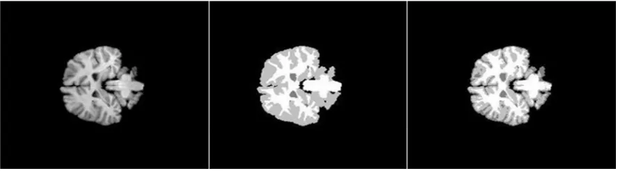
In the present study, experiments were also conducted to apply the FFCM to real 3D MRI brain images downloaded from the IBSR [27]. This set comprised 20 normal MRI brain images with ground truth images manually segmented by experts. These images are T1-weighted with a resolution of 256 x 256 x 64, and the size of voxel is 1.17 x 1.17 x 3.1 mm3, downloaded from many 1.5-Tesla GE/Siemens MRI scanners. The reasons for choosing this type of images is the difficulty encountered in segmentation due to variations in shape complexity, low signal to noise ratio and severe spatial intensity non-uniformity [29]. The first step in this experiment was to remove the undesirable tissues such as bone, fat and skull from the original and from the ground truth images to arrive at the region of interest. Figure 6 illustrates this process.
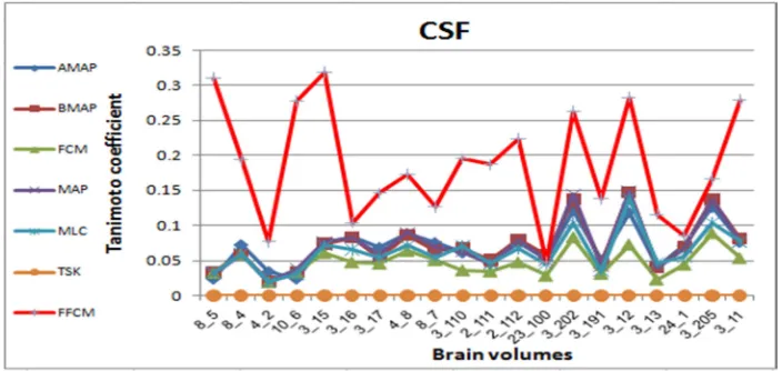
The accuracy rate was computed based on the similarity between the ground truth image and a segmented image by FFCM. The Tanimoto coefficient T ∈ $0,1& [30] was the quantization index used in this part of the study. The Tanimoto coefficient T is used as an overlap metric and is reported on the IBSR website. It is computed as follows:
K |O ∩ Q||O ∪ Q| , 14
where A represents the number of voxels in the ground truth and B represents the number of voxels in the FFCM segmented image. The best similarity between A and B is the maximum value of T, and the best value for T equals 1. Figure 7 shows, from left to right respectively, the original image, ground truth image and image segmented by FFCM.
ISSN: 1992-8645 www.jatit.org E-ISSN: 1817-3195
From Figs. 8, 9 and 10 and Table 7, it can be seen that the FFCM outcomes are much better than those produced by all the other algorithms in the case of the WM tissue segmentations. Moreover, FFCM is also better than the algorithms from the IBSR website in the case of the GM tissue segmentations, but it is not better than two state-of-the-art methods (MPM-MAP, AMS). For CSF tissue, the FFCM results are better than all algorithms except for one of the state-of-the-art methods, (Fixed wMS). Finally, the FFCM outcomes for WM tissues segmentation are better than those for CSF and GM tissue segmentation. This is due to MRI images artifacts and the intensity levels similarity between CSF and GM.
5.6 FFCM execution time
The execution time to segment MRI images (simulated and real) by FFCM took more than one hour; however, the simplified process for the objective function described in Section 4.1 reduces the execution time for the segmentation of MRI images (simulated and real) by FFCM to around 4 s. Thus, this process minimizes the
execution time and makes the FFCM algorithm more efficient.
[image:14.612.88.537.392.491.2]
Fig 6. Tissue removal steps from left to right, original volume 16_3 (slice #22), ground truth, region of interest.
[image:14.612.90.534.542.665.2]Fig 7b. From Left To Right, Original Volume (8_4), Ground Truth Volume (8_4), And Segmented Volume (8_4) By FFCM.
Fig 7c .From Left To Right, Original Volume (205_3), Ground Truth Volume (205_3), And Segmented Volume (205_3) By FFCM.
[image:15.612.131.483.416.583.2]ISSN: 1992-8645 www.jatit.org E-ISSN: 1817-3195
[image:16.612.117.501.290.443.2]
Fig. 9. FFCM Tanimoto Coefficient (T) For The 20 IBSR Images Compared With Other Algorithms For WM.
Fig 10. FFCM Tanimoto Coefficient (T) For The 20 IBSR Images Compared With Other Algorithms For GM.
Table 7. Tanimoto Coefficient (T) Outcome Averages For FFCM Segmentation And Other Methods.
Method CSF GM WM
Adaptive MAP 0.069 0.564 0.567
Biased MAP 0.071 0.558 0.562
FCM 0.048 0.473 0.567
MAP 0.071 0.55 0.554
MLC 0.062 0.535 0.551
TSK means 0.049 0.477 0.571
AFR 0.092 0.557 0.587
Fixed wMS 0.21 0.594 0.628
MPM-MAP N/A 0.662 0.683
AMS N/A 0.683 0.691
FFCM 0.186 0.600 0.727
6. CONCLUSION
This research proposed a new clustering approach based on the hybridization of firefly algorithm (FA) and fuzzy c-means algorithm(FCM) called (FFCM) to segment MRI brain images. this
[image:16.612.142.470.495.653.2]employed as an MRI image segmentation method and the outcomes of the segmentation of simulated and real MRI brain images indicated the efficiency of the proposed algorithm in comparison with state-of-the-art segmentation algorithms and the randomly initialized FCM segmentation
ACKNOWLEDGEMENT
This research is based on two research grants from Ministry of Science, Technology and Innovation, Malaysia entitled “Sciencefund 01-01-02-SF0694 Spiking-LVQ Network For Brain Tumor Detection” and Arus Perdana Fund AP-2012-019 entitled “Automated Medical Imaging Diagnostic Based on Four Critical Diseases: Brain, Breast, Prostate and Lung Cancer” . We have obtained Ethics approval entitled “FF-342-2012 Imaging Processing of the Brain Tumor Using LVQ Classifier” from PPUKM or UKM Medical Canter, Malaysia for collecting and conducting experiments on MRI Brain Tumor patient’s record.
REFERENCES
[1] J. A. Richards, Remote sensing digital image analysis: an introduction: Springer, 2013. [2] M. A. Balafar, et al., "Review of brain MRI
image segmentation methods," Artificial Intelligence Review, vol. 33, pp. 261-274, 2010.
[3] D. L. Pham, et al., "Current methods in medical image segmentation 1," Annual review of biomedical engineering, vol. 2, pp. 315-337, 2000.
[4] J. C. Bezdek, Pattern Recognition with Fuzzy Objective Function Algorithms: Kluwer Academic Publishers, 1981.
[5] J. Kang, et al., "Novel modified fuzzy c-means algorithm with applications," Digital Signal Processing, vol. 19, pp. 309-319, 2009.
[6] P. Hore, et al., "A scalable framework for segmenting magnetic resonance images," Journal of signal processing systems, vol. 54, pp. 183-203, 2009.
[7] O. d. Alia, et al., "A hybrid harmony search algorithm for MRI brain segmentation," Evolutionary Intelligence, vol. 4, pp. 31-49, 2011/03/01 2011.
[8] A. Abraham, et al., "Swarm Intelligence Algorithms for Data Clustering," in Soft Computing for Knowledge Discovery and Data Mining, O. Maimon and L. Rokach, Eds., ed: Springer US, 2008, pp. 279-313.
[9] D. Karaboga, et al., "A comprehensive survey: artificial bee colony (ABC) algorithm and applications," Artificial Intelligence Review, pp. 1-37, 2012/03/01 2012.
[10] G. Ingram and T. Zhang, "Overview of Applications and Developments in the Harmony Search Algorithm," in Music-Inspired Harmony Search Algorithm. vol. 191, Z. Geem, Ed., ed: Springer Berlin Heidelberg, 2009, pp. 15-37.
[11] P. M. Kanade and L. O. Hall, "Fuzzy Ants and Clustering," Systems, Man and Cybernetics, Part A: Systems and Humans, IEEE Transactions on, vol. 37, pp. 758-769, 2007.
[12] S. Z. Selim and K. Alsultan, "A simulated annealing algorithm for the clustering problem," Pattern Recognition, vol. 24, pp. 1003-1008, 1991.
[13] R. H. Sheikh, et al., "Genetic Algorithm Based Clustering: A Survey," in Emerging Trends in Engineering and Technology, 2008. ICETET '08. First International Conference on, 2008, pp. 314-319.
[14] L. O. Hall, et al., "Clustering with a genetically optimized approach,"
Evolutionary Computation, IEEE
Transactions on, vol. 3, pp. 103-112, 1999. [15] K. S. Al-Sultan and C. A. Fedjki, "A tabu
search-based algorithm for the fuzzy clustering problem," Pattern Recognition, vol. 30, pp. 2023-2030, 1997.
[16] T. Hassanzadeh and M. R. Meybodi, "A new hybrid approach for data clustering using firefly algorithm and K-means," in Artificial Intelligence and Signal Processing (AISP), 2012 16th CSI International Symposium on, 2012, pp. 007-011.
[17] L. Lili, et al., "A Novel Fuzzy Clustering Based on Particle Swarm Optimization," in Information Technologies and Applications in Education, 2007. ISITAE '07. First IEEE International Symposium on, 2007, pp. 88-90.
[18] X.-S. Yang, "Firefly algorithm, stochastic test functions and design optimisation," International Journal of Bio-Inspired Computation, vol. 2, pp. 78-84, 2010. [19] J. Senthilnath, et al., "Clustering using firefly
ISSN: 1992-8645 www.jatit.org E-ISSN: 1817-3195
[20] D. Karaboga and C. Ozturk, "A novel clustering approach: Artificial Bee Colony (ABC) algorithm," Applied Soft Computing, vol. 11, pp. 652-657, 2011.
[21] X.-S. Yang, Nature-Inspired Metaheuristic Algorithms: Luniver Press, 2008.
[22] A. K. Jain, et al., "Data clustering: a review," ACM Comput. Surv., vol. 31, pp. 264-323, 1999.
[23] Q. W. Bsoul and M. Mohd, "Effect of ISRI stemming on similarity measure for arabic document clustering," presented at the Proceedings of the 7th Asia conference on Information Retrieval Technology, Dubai, United Arab Emirates, 2011.
[24] R. J. Hathaway and J. C. Bezdek, "Optimization of clustering criteria by reformulation," Fuzzy Systems, IEEE Transactions on, vol. 3, pp. 241-245, 1995. [25] J. C. Bezdek, et al., Fuzzy Models and
Algorithms for Pattern Recognition and
Image Processing: Springer
Science+Business Media, Incorporated, 2005.
[26] BainWeb. (Nov 2003, simulated brain database Mcconnell Brain Imaging Centre Montreal Neurological Institute Mcgill
University. Available:
http://www.bic.mni.mcgill.ca/brainweb [27] IBSR. (Sep 2005, : internet brain
segmentation repository. Technical report, Massachusetts General Hospital, Center for Morphometric Analysis. Available: http://neuro-www.mgh.harvard.edu/cma/ibsr/ [28] A. Ben-Hur and I. Guyon, "Detecting stable clusters using principal component analysis," in Functional Genomics, ed: Springer, 2003, pp. 159-182.
[29] Z. Peng, "Segmentation of white matter, gray matter, and CSF from MR brain images and extraction of vertebrae from MR spinal images," University of Cincinnati, 2006. [30] R. O. Duda, et al., Pattern classification: