Simulation of snow accumulation and melt in needleleaf forest environments

(1)

Hydrol. Earth Syst. Sci., 14, 925–940, 2010 www.hydrol-earth-syst-sci.net/14/925/2010/ doi:10.5194/hess-14-925-2010

Hydrology and

Earth System

Sciences

Simulation of snow accumulation and melt in needleleaf forest

environments

C. R. Ellis, J. W. Pomeroy, T. Brown, and J. MacDonald

Centre for Hydrology, University of Saskatchewan, 117 Science Place, Saskatoon, Saskatchewan, S7N 5C8, Canada Received: 15 January 2010 – Published in Hydrol. Earth Syst. Sci. Discuss.: 9 February 2010

Revised: 5 May 2010 – Accepted: 7 May 2010 – Published: 14 June 2010

Abstract. Drawing upon numerous field studies and

mod-elling exercises of snow processes, the Cold Regions Hydro-logical Model (CRHM) was developed to simulate the four season hydrological cycle in cold regions. CRHM includes modules describing radiative, turbulent and conductive en-ergy exchanges to snow in open and forest environments, as well as account for losses from canopy snow sublimation and rain evaporation. Due to the physical-basis and rigorous testing of each module, there is a minimal need for model calibration. To evaluate CRHM, simulations of snow accu-mulation and melt were compared to observations collected at paired forest and clearing sites of varying latitude, eleva-tion, forest cover density, and climate. Overall, results show that CRHM is capable of characterising the variation in snow accumulation between forest and clearing sites, achieving a model efficiency of 0.51 for simulations at individual sites. Simulations of canopy sublimation losses slightly overesti-mated observed losses from a weighed cut tree, having a model efficiency of 0.41 for daily losses. Good model perfor-mance was demonstrated in simulating energy fluxes to snow at the clearings, but results were degraded from this under forest cover due to errors in simulating sub-canopy net long-wave radiation. However, expressed as cumulative energy to snow over the winter, simulated values were 96% and 98% of that observed at the forest and clearing sites, respectively. Overall, the good representation of the substantial variations in mass and energy between forest and clearing sites suggests that CRHM may be useful as an analytical or predictive tool for snow processes in needleleaf forest environments.

Correspondence to: C. R. Ellis

([email protected])

1 Introduction

Needleleaf forests dominate much of the mountain and bo-real regions of the northern hemisphere where snowmelt is the most important hydrological event of the year (Gray and Male, 1981). The retention of foliage by evergreen needle-leaf tree species during winter acts to decrease snow accumu-lation via canopy interception losses (Schmidt, 1991; Lund-berg and Halldin, 1994; Pomeroy et al., 1998a) and greatly modify energy exchanges to snow (Link and Marks, 1999; Gryning and Batchvarova, 2001; Ellis et al., 2010). How-ever, forest cover is often discontinuous, containing clear-ings of varying dimensions which may differ considerably in snow accumulation (McNay, 1988) and melt characteristics (Metcalfe and Buttle, 1995). As such, management of water derived from forest snowmelt is expected to benefit from the effective prediction of snow accumulation and melt in both forest and open environments.

(2)

926 C. R. Ellis et al.: Simulation of forest snow accumulation and melt have often made appeal to physically-based “ice-sphere”

models (e.g. Schmidt, 1991) which adjust sublimation losses from a single, small ice-sphere for the decreased exposure of canopy snow to the atmosphere. Such methods have been shown to well approximate canopy sublimation losses over multiple snowfall events through the coupling of the multi-scale sublimation model to a needleleaf forest interception model (Pomeroy et al., 1998a).

Alongside interception effects, needleleaf forest cover also influences energy exchanges to snow. The forest layer acts to effectively decouple the above-canopy and sub-canopy at-mospheres, resulting in a large suppression of turbulent en-ergy fluxes (Harding and Pomeroy, 1996; Link and Marks, 1999). Consequently, energy to sub-canopy snow is dom-inated by radiation; itself modified by the canopy through the shading of shortwave irradiance while increasing long-wave irradiance from canopy thermal emissions (Link et al., 2004; Sicart et al., 2004; Pomeroy et al., 2009). Forest cover may also affect sub-canopy shortwave radiation by altering snow surface albedo through deposition of forest litter on snow (Hardy et al., 2000; Melloh et al., 2002), or by influ-encing energy-controlled snow metamorphism rates (Ellis et al., 2010). As such, simulations of forest effects on energy to snow have largely focused on the adjustment of shortwave and longwave fluxes (Hardy et al., 2004; Essery et al., 2008; Pomeroy et al., 2009), although methods estimating turbu-lent energy transfer in forests have also been described (Hell-str¨om, 2000; Gelfan et al., 2004).

Since the first successful demonstration of snowmelt simulation using an energy-balance approach by Ander-son (1976), numerous such snowmelt models have developed (e.g. EBSM, Gray and Landine, 1988; SNTHERM, Jordan, 1991; SHAW, Flerchinger and Saxton, 1989; Snobal, Marks et al., 1999). Due to the differing objective specific to each model, there is considerable variation in the detail to which snow energetics may be described, as well as forcing data and parameterization requirements. In general, more sophis-ticated snowmelt models possess information requirements that may prohibit their successful employment in more re-mote environments, where forcing data and parameter in-formation is typically lacking or poorly approximated. In-stead, more basic models that maintain a physically-based representation of forest snow processes in cold regions are expected to be better suited for such environments.

Although much focus has been placed on simulating for-est snow accumulation and melt processes separately, fewer simulations over the entire snow accumulation and melt pe-riod have been demonstrated. To this end, this paper outlines and evaluates the simulation of snow accumulation and melt in paired forest and clearing sites of varying forest cover den-sity and climate using the Cold Regions Hydrological Model (CRHM). CRHM is a deterministic model of the hydrologi-cal cycle containing process algorithms (modules) developed from field investigations in cold region environments, with modest data and parameter requirements. This paper

exam-ines the potential for CRHM to be used to analyze and pre-dict how changes in climate and forest-cover may affect snow processes in cold region forests.

2 Model description

Described in detail by Pomeroy et al. (2007), CRHM oper-ates through interaction of its four main components: (1) ob-servations, (2) parameters, (3) modules, and (4) variables and states. The description of each component below focuses on the requirements of CRHM for forest environments:

1. Observations: CRHM requires the following meteo-rological forcing data for each simulation timestep, t

(units in [ ]):

a air temperature ,Ta[◦C];

b humidity, either as vapour pressure,ea[kPa] or rel-ative humidity, RH [%];

c precipitation,P [kg m−2_];

d wind speed, observed either above, or within the canopy,u[m s−1_];

e shortwave irradiance,K↓[W m−2_{] (in the absence} of observations,K↓may be estimated fromTa); f longwave irradiance, L↓[W m−2_{] (in the absence}

of observations,L↓may be estimated fromTaand

ea).

2. Parameters: provides a physical description of the site, including latitude, slope and aspect, forest cover den-sity, height, species, and soil properties. In CRHM, for-est cover need only be quantified by an effective leaf area index (LAI’) and forest height (h); the forest sky view factor (v) may be specified explicitly or estimated from LAI’. The heights at which meteorological forcing data observations are collected are also specified here. 3. Modules: algorithms implementing the particular

hy-drological processes are selected here by the user. 4. Initial states and variables: specified within the

appro-priate module.

3 Modules

The following provides a general outline of the main modules and associated algorithms in CRHM.

3.1 Observation module

To allow for the distribution of meteorological observations away from the point of collection, appropriate corrections are applied to observations within the observation module. These include the correction of air temperature, humidity,

(3)

C. R. Ellis et al.: Simulation of forest snow accumulation and melt 927 and the amount and phase of precipitation for elevation, as

well as correction of shortwave and longwave irradiance for topography.

3.2 Snow mass-balance module

In CRHM, snow is conserved within a single defined spatial unit, with changes in mass occurring only through a diver-gence of incoming and outgoing fluxes. In clearing environ-ments, snow water equivalent (SWE) [kg m−2] at the ground may be expressed by the following mass-balance of vertical and horizontal snow gains and losses

SWE=SWEo+(Ps+Pr+Hin−Hout−S−M)t (1) wheret is the time step in the model calculation, SWEois the antecedent snow water equivalent [kg m−2],Ps andPr are the respective snowfall and rainfall rates,Hin is the in-coming horizontal snow transport rate,Houtis the outgoing horizontal snow transport rate,Sis the sublimation loss rate, andM is the melt loss rate [all units kg m−2_t−1_{]. In forest} environments Eq. (1) is modified to

SWE=SWEo+(Ps−(Is−Ul)+Pr−(Ir−Rd)−M)t (2) in whichIs is canopy snowfall interception rate, Ul is the rate of canopy snow unloading,Ir is the canopy rainfall in-terception rate, and Rd is the rate of canopy rain drip [all units kg m−2t−1].

The amount of snowfall intercepted by the canopy is de-pendent on various physical factors, including tree species, forest density, and the antecedent intercepted snowload (Is,o) [kg m−2_{]. In CRHM, a dynamic canopy snow-balance is} cal-culated, in which the amount of snow interception (Is)is de-termined by

Is =(Is∗−Is,o)(1−e−ClPst /I

∗

s₎ ₍₃₎

whereCl is the “canopy-leaf contact area” per unit ground [], and I*s is the species-specific maximum intercepted snowload [kg m−2], which is determined as a function of the mean maximum snowload per unit area of branch, S

[kg m−2], the density of falling snow,ρs[kg m−3], and LAI0 by

I_s∗=S

0.27+46 ρs

LAI0. (4)

Sublimation of intercepted snow is estimated following the Pomeroy et al. (1998) multi-scale model, in which the subli-mation rate coefficient for intercepted snow,Vi[s−1], is mul-tiplied by the intercepted snowload to give the canopy subli-mation flux,qe[kg m−2s−1], i.e.

qe =ViIs. (5)

Here,Vi is determined by adjusting the sublimation flux for a 500 µm radius ice-sphere,Vs[s−1], by the intercepted snow exposure coefficient,Ce[], i.e.

Vi =VsCe, (6)

in whichCeis defined by Pomeroy and Schmidt (1993) as

Ce =k

_I

s

I∗_s

−F

. (7)

wherekis a dimensionless coefficient indexing the shape of intercepted snow (i.e. age and structure) andF is an exponent value of approximately 0.4. The ventilation wind speed of intercepted snow may be set as an observed within-canopy wind speed, or approximated from above-canopy wind speed by

uξ =uhe−ψ ξ (8)

whereuξ [m s−1] is the estimated within-canopy wind speed at a fractionξ of the entire forest depth [], uh is the wind speed at the canopy top [m s−1], andψ is the canopy wind speed extinction coefficient [], which is determined as a lin-ear function of LAI’ for various needleleaf species (Eagle-son, 2002). Unloading of intercepted snow to the sub-canopy snowpack is calculated as an exponential function of time following Hedstrom and Pomeroy (1998). Additional un-loading resulting from melting intercepted snow is estimated by specifying a threshold ice-bulb temperature (Tb)in which all intercepted snow is unloaded when exceeded for three hours (Gelfan et al., 2004).

3.3 Rainfall interception and evaporation module

Although the overall focus of this manuscript is that of snow-forest interactions, winter rainfall may represent substan-tial water and energy inputs to snow. The fraction of rain-fall to sub-canopy snow received as direct throughrain-fall is as-sumed to be inversely proportional to the fractional hori-zontal canopy coverage (Cc)[]. All other rainfall is inter-cepted by the canopy, which may be lost via evaporation (E) [kg m−2t−1] or dripped to the sub-canopy if the canopy rain storage (CR) [mm] exceeds the maximum canopy stor-age (Smax) [mm]. Here, direct throughfall and drip to the sub-canopy are added to the water equivalent of the snow-pack. The intercepted rainload (Ir,o)[kg m−2] in CRHM is estimated using a simplified Rutter model approach (Rutter, 1971) in which a single storage is determined and scaled for sparse canopies by Cc (e.g. Valente et al., 1997). Evapo-ration from a fully-wetted canopy (Ep)[kg m−2t−1] is cal-culated using the Penman-Monteith combination equation (Monteith, 1965) for the case of no stomatal resistance, i.e.

E=CcEp forCR=Smax. (9)

For partially-wetted canopies E is reduced in proportion to the degree of canopy saturation, i.e.

(4)

928 C. R. Ellis et al.: Simulation of forest snow accumulation and melt

3.4 Snow energy-balance module

Energy to snow (Q*) is resolved in CRHM as the sum of radiative, turbulent, advective and conductive energy fluxes to snow, i.e.

K∗ +L∗ +Qh+Qe+Qg+Qp=

dU

dt +Qm=Q∗ (11)

whereQmis the energy for snowmelt, dU/dtis the change in internal (stored) energy of snow,K∗andL∗are net short-wave and longshort-wave radiations, respectively,Qh andQe are the net sensible and latent heat turbulent fluxes, respectively,

Qg is the net ground heat flux, andQp is the energy from rainfall advection [all units MJ m−2t−1]. In Eq. (11), posi-tive magnitudes represent energy gains to snow and negaposi-tive magnitudes are energy losses. The amount of melt (M) is calculated fromQmby

M= Qm

ρwB λf

(12)

whereρw is the density of water [kg m−3],Bis the fraction of ice in wet snow [∼0.95−0.97], andλf is the latent heat of fusion for ice [MJ kg−1].

3.4.1 Adjustment of energy fluxes to snow for needleleaf forest cover

For the purpose of brevity, the following section outlines the algorithms in CRHM estimating energy fluxes in forest envi-ronments only. For an overview of energy flux estimations by CRHM in open environments, refer to Pomeroy et al. (2007).

Shortwave radiation to forest snow

In CRHM, net shortwave radiation to forest snow (K∗_f)

is equal to the above-canopy irradiance (K↓) transmitted through the canopy less the amount reflected from snow, ex-pressed here as

K∗_f =K↓τ (1−αs) (13)

in whichαsis the snow surface albedo [], the decay of which is approximated as a function of time subsequent to a snow-fall event, and τ is the forest shortwave transmittance [], which is estimated by the following variation of Pomeroy and Dion’s (1996) formulation (Pomeroy et al., 2009)

τ =e−

1.081θcos(θ )LAI‘

sin(θ ) ₍₁₄₎

whereθis the solar angle above the horizon [radians].

Longwave radiation to forest snow

As stated previously, longwave irradiance to forest snow (L↓_f)may be enhanced relative to that in the open as the

result of thermal emissions from the canopy. Simulation of

L↓_fis made as the sum of sky and forest longwave emis-sions weighted by the sky view factor (v), i.e.

L↓_f=vL↓ +(1−v)εfσ Tf4. (15)

Here,εf is the forest thermal emissivity [],σ is the Stefan-Boltzmann constant [W m−2K−4], andTf is the forest tem-perature [K]. Longwave exitance from snow (L↑) is deter-mined by

L↑=εsσ Ts4 (16)

whereεs is the thermal emissivity of snow [], andTsis the snow surface temperature [K] which is resolved using the longwave psychrometric formulation by Pomeroy and Es-sery (2010):

Ts=Ta+

εs L↓ −σ Ta4

+λs(wa−ws)ρa/ra

4εsσ Ta3+(cp+λs1)ρa/ra

(17) wherewaandwsare the specific and saturation mixing ratios [],ρa is the air density [kg m−3],cpis the specific heat ca-pacity of air [J kg−1K−1],λsis the latent heat of sublimation [MJ kg−1],rais the aerodynamic resistance [s m−1], and1is the slope of the saturation vapour pressure curve [kPa K−1].

Sensible (Qh)and latent (Qe)heat fluxes

Determination ofQhandQein open and forest sites are made using the following semi-empirical formulations developed by Gray and Landine (1988):

Qh=-0.92+0.076umean+0.19Tmax (18)

Qe=0.08(0.18+0.098umean) (6.11−10eamean) (19) whereumeanis the mean daily wind speed [m s−1],Tmaxis the maximum daily air temperature [◦C], and eamean is the mean daily vapour pressure [kPa]. For the case of rainfall to melting snow (i.e.Ts=0◦C), the energy delivered to the snowpack via rainfall advection (Qp)is given by

Qp =4.2×10−3(Pr−Ir)Tr (20)

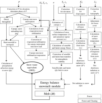
whereTr is the rainfall temperature [◦C], which is approxi-mated byTa. The primary mass and energy balance calcula-tion routines for both forest and clearing environments within CRHM are summarized in Fig. 1.

4 Model application

Simulations of snow accumulation and melt using CRHM were performed at five paired forest and clearing sites of varying location, climate, forest species, and forest cover density (Table 1). With the exception of the Marmot Creek sites, all simulations were performed as part of the second

(5)

C. R. Ellis et al.: Simulation of forest snow accumulation and melt 929

Meteorological forcing observations: shortwave irradiance (K↓) longwave irradiance (L↓) precipitation

(P), wind speed (u), air temperature (Ta), humidity (ea):

Energy balance snowmelt module

Calculation of longwave exitance from snow

(L↑) Estimation of

canopy u

Correction for elevation

Calculation of snow surface temperature (Ts)

and saturation vapour pressure (es)

Calculation of sensible and latent energy fluxes

Correction of sensible and latent heat transfers

for atmospheric stability

Sensible (Qh) and latent (Qe) heat to snow Rain/snowfall to

snowpack

Calculation of precipitation advection energy

to snow (Qp) P

Correction of Pfor elevation; determine phase of P

Snow water equivalent

(SWE)

Melt (M)

u Ta, ea K↓ L↓

Correction for topography

Calculation of forest transmittance

(τ)

Calculation of reflection from snow

(αs) Correction

for slope/aspect

Net shortwave radiation to

snow (K*)

Adjustment for forest

cover

Net shortwave radiation to

snow (L*)

Calculation of snow surface temperature

(Ts) Canopy rain/snow

interception

Direct throughfall

Calculation of rain evaporation/snow

sublimation K↓,

Canopy snow unloading/rain

drip

Correction of evaporation/sublimation

for canopy intercepted rain/snow load

Ta, ea

Canopy rain/snow sublimation/evaporation

loss

Net radiation to snow (Qn)

[image:5.595.128.469.61.403.2]

Forest and Clearing Forest

Fig. 1. Schematic outlining the major mass and energy calculations involved in the forest component of the Cold Regions Hydrological Model (CRHM).

snow model inter-comparison project (SnoMIP2) (Rutter et al., 2009; Essery et al., 2009). This initiative involved the off-line simulation of snow accumulation and melt in paired forest and nearby clearing sites located in Canada, Switzer-land, FinSwitzer-land, Japan and the United States. Hourly standard meteorological forcing data, site descriptions, and initial states were provided to each participant by the SnoMIP2 facilitators. All simulations in SnowMIP2 were executed “blindly” with the exception of the Switzerland location for the 2002–2003 season where SWE field data were provided to allow for the option of model calibration. Location, to-pography and forest cover descriptions for all sites are given in Table 1, and site pictures in Fig. 2. Simulations of snow accumulation and melt were performed for both forest and adjacent forest clearing sites at each location for the period extending from 1 October to approximately 1 June. For each simulation timestep, appropriate energy, mass, and state vari-ables were outputted by the model.

4.1 Simulation of snow accumulation and melt

4.1.1 Evaluation of model performance

Simulations of snow accumulation and melt by CRHM were evaluated in terms of the ability of representing:

1. the variation in mean and maximum seasonal SWE ob-served between all sites; and

2. the timing and quantity of SWE accumulation and melt at individual sites.

(6)

Alptal, Switzerland forest (left) and clearing (right).

BERMS, Saskatchewan, Canada forest (left) and clearing (right).

Fraser, Colorado, USA forest (left) and clearing (right).

Marmot Creek, Alberta, Canada pine forest (left) and clearing (right).

Marmot Creek, Alberta, Canada spruce forest showing the suspended spruce tree (left), the spruce clearing (centre) and reference radiation tower at the spruce clearing (right).

Figure 2. Photographs of meteorological stations located at forest and clearing sites at Alptal,

Switzerland; BERMS, Saskatchewan, Canada; Fraser, Colorado, USA; and pine and spruce sites

at Marmot Creek, Alberta, Canada (with the exception of the Marmot Creek sites, site

[image:6.595.160.438.70.603.2]

photographs were provided by the SnowMIP2 facilitators).

Fig. 2. Photographs of meteorological stations located at forest and clearing sites at Alptal, Switzerland; BERMS, Saskatchewan, Canada; Fraser, Colorado, USA; and pine and spruce sites at Marmot Creek, Alberta, Canada (with the exception of the Marmot Creek sites, site photographs were provided by the SnowMIP2 facilitators).

(7)

[image:7.595.80.511.108.377.2]

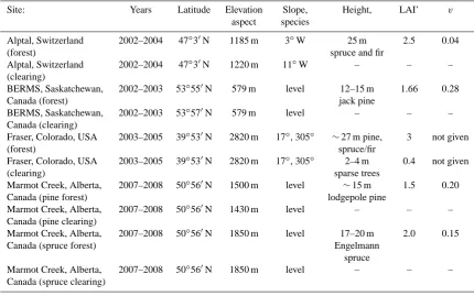
Table 1. Location, topography, and forest cover descriptions of paired clearing and forest sites used in simulations of snow accumulation and melt.

Site: Years Latitude Elevation Slope, Height, LAI’ v

aspect species

Alptal, Switzerland 2002–2004 47◦30N 1185 m 3◦W 25 m 2.5 0.04

(forest) spruce and fir

Alptal, Switzerland 2002–2004 47◦30N 1220 m 11◦W – – –

(clearing)

BERMS, Saskatchewan, 2002–2003 53◦550N 579 m level 12–15 m 1.66 0.28

Canada (forest) jack pine

BERMS, Saskatchewan, 2002–2003 53◦570N 579 m level – – –

Canada (clearing)

Fraser, Colorado, USA 2003–2005 39◦530N 2820 m 17◦, 305◦ ∼27 m pine, 3 not given

(forest) spruce/fir

Fraser, Colorado, USA 2003–2005 39◦530N 2820 m 17◦, 305◦ 2–4 m 0.4 not given

(clearing) sparse trees

Marmot Creek, Alberta, 2007–2008 50◦560N 1500 m level ∼15 m 1.5 0.20

Canada (pine forest) lodgepole pine

Marmot Creek, Alberta, 2007–2008 50◦560N 1430 m level – – –

Canada (pine clearing)

Marmot Creek, Alberta, 2007–2008 50◦560N 1850 m level 17–20 m 2.0 0.15

Canada (spruce forest) Engelmann

spruce

Marmot Creek, Alberta, 2007–2008 50◦560N 1850 m level – – –

Canada (spruce clearing)

Alpt

al 2

00

2-03 (c

lear

ing)

Alpt

al 2

00

2-03 (f

ores

t)

Alpt

al 2

00

3-04 (c

lear

ing)

Alpt

al 2

00

3-04 (f

ores t) BER MS 2002 -03 (cle arin g) BER MS 2002 -03 (for est) Fras

er 2

00

3-04 (c

lear

ing)

Fras

er 2

00

3-04 (f

ores

t)

Fras

er 2

00

4-05 (c

lear

ing)

Fras

er 2

00

4-05 (f

ores t) Mar mot 200 7-08 (pin

e cl

eari ng) Mar mot 200 7-08 (pin

e fo rest ) Mar mot 200 7-08 (spr uce clea ring ) Mar mot 200 7-08 (spr uce fore st) SW E [ kg m -2] 0 50 100 150 200 250 300

[image:7.595.307.439.483.536.2]

mean SWE (observed) mean SWE (simulated) maximum SWE (observed) maximum SWE (simulated)

Figure 3.

Fig. 3. Observed and simulated mean and maximum snow water equivalent (SWE) accumulations at forest and clearing sites.

quantification of the absolute unit error between simulations and observations. Here, the MB is calculated as

MB=

n

P

i=1

xsim

n

P

i=1

xobs

(21)

where xsim and xobs are the respective simulated and ob-served values at a given timestep fornnumber of paired sim-ulated and observed values. Accordingly, MB values less than 1 signify an overall under-prediction by the model, and values greater than 1 an overall over-prediction by the model. The model efficiency index (ME) is given by

ME=1−     n P

i=1

(xsim−xobs)2

n

P

i=1

(xobs−xavg)2



  

(22)

wherexavg is the mean value of n number of xobs values. In Eq. (22), model efficiency increases as the ME index ap-proaches 1, which represents a perfect match between simu-lations and observations; 0 indicates an equal efficiency be-tween simulations and the xavg, with increasingly negative values signifying a progressively superior estimation by the

xavg. The root mean square error (RMSE) is determined by

RMSE= v u u t 1 n n X

i=1

(8)

[image:8.595.50.283.200.582.2]

Table 2. Model bias index (MB), model efficiency index (ME), and root mean square error (RMSE) of simulated mean and maximum snow water equivalent (SWE) at clearing sites, forest sites, and all sites.

Mean SWE Maximum SWE

Clearing Forest All Clearing Forest All

Model bias (MB) 0.99 0.94 0.97 0.94 0.94 0.94

Model efficiency (ME) 0.97 0.93 0.96 0.92 0.87 0.90

Root mean square error (RMSE) [kg m−2] 16.0 16.1 16.0 27.0 21.6 24.4

Alptal (2002-03)

0 50 100 150 200 250 300

SW

E

[

k

g

m

-2]

0 50 100 150 200 250 300

Days after October 1

Alptal (2003-04)

0 50 100 150 200 250 300

SW

E

[k

g

m

-2]

0 50 100 150 200 250 300 350

BERMS (2002-03)

0 50 100 150 200 250

S

W

E

[k

g

m

-2]

0 20 40 60 80

Fraser (2003-04)

0 50 100 150 200 250 300

SW

E

[k

g

m

-2]

0 50 100 150 200 250

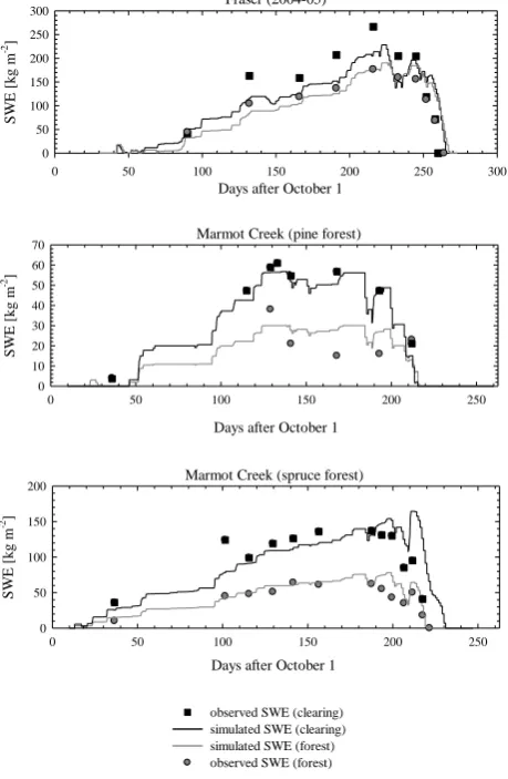
Fig. 4. Time series of observed and simulated SWE at paired forest and clearing sites.

Simulation of mean and maximum winter SWE at all sites

Among all sites, considerable variation in mean and maxi-mum seasonal SWE was observed, with mean SWE rang-ing from 20 to 160 kg m−2, and maximum SWE from 29 to

Fraser (2004-05)

0 50 100 150 200 250 300

SW

E

[k

g

m

-2]

0 50 100 150 200 250 300

0 50 100 150 200 250

SW

E

[

kg

m

-2]

0 10 20 30 40 50 60

70 Marmot Creek (pine forest)

0 50 100 150 200 250

SW

E

[k

g

m

-2]

0 50 100 150

200 Marmot Creek (spruce forest)

Alptal, Switzerland (2002-03)

0 50 100 150 200 250 300

S

W

E

(

m

)

0 50 100 150 200 250 300 observed SWE (clearing) simulated SWE (clearing) simulated SWE (forest) observed SWE (forest)

Figure 4.

Fig. 4. Continued.

295 kg m−2_{. Large variations in SWE were also observed} be-tween paired forest and clearings, with forest accumulations ranging from approximately 30% of the clearing accumula-tion at the Alptal locaaccumula-tion (2003–2004) to near even accumu-lations at the BERMS location.

Simulated and observed mean and maximum SWE at all sites are shown in Fig. 3 with model performance in-dex values given in Table 2. Here, simulations exhibit a small systematic under-prediction of mean SWE for all sites (MB=0.97), with a slightly greater under-prediction for the

[image:8.595.311.541.204.556.2]

(9)

[image:9.595.159.434.98.322.2]

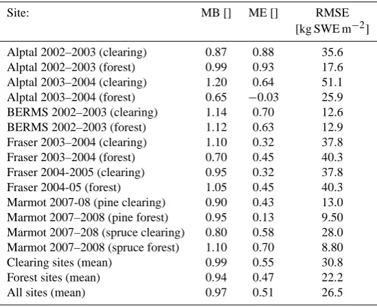
Table 3. Determined model bias index (MB), model efficiency index (ME), and root mean square error (RMSE) for simulations of snow water equivalent (SWE) at individual sites.

Site: MB [] ME [] RMSE

[kg SWE m−2]

Alptal 2002–2003 (clearing) 0.87 0.88 35.6 Alptal 2002–2003 (forest) 0.99 0.93 17.6 Alptal 2003–2004 (clearing) 1.20 0.64 51.1 Alptal 2003–2004 (forest) 0.65 −0.03 25.9 BERMS 2002–2003 (clearing) 1.14 0.70 12.6 BERMS 2002–2003 (forest) 1.12 0.63 12.9 Fraser 2003–2004 (clearing) 1.10 0.32 37.8 Fraser 2003–2004 (forest) 0.70 0.45 40.3 Fraser 2004-2005 (clearing) 0.95 0.32 37.8

Fraser 2004-05 (forest) 1.05 0.45 40.3

Marmot 2007-08 (pine clearing) 0.90 0.43 13.0 Marmot 2007–2008 (pine forest) 0.95 0.13 9.50 Marmot 2007–208 (spruce clearing) 0.80 0.58 28.0 Marmot 2007–2008 (spruce forest) 1.10 0.70 8.80

Clearing sites (mean) 0.99 0.55 30.8

Forest sites (mean) 0.94 0.47 22.2

All sites (mean) 0.97 0.51 26.5

forest sites. In comparison, a greater under-prediction of maximum SWE at all sites was realised (MB=0.94). Yet, the high ME value indicates CRHM well represented the variability in mean and maximum SWE accumulations be-tween sites. Similar to MB results, the ME shows supe-rior prediction of mean SWE to that of maximum SWE, as well as better prediction for clearing sites relative to forest sites. However, due to less snow at the forest sites, the lower MB and ME indexes at the forest sites translate into simi-lar magnitudes of absolute error to that at the clearings (i.e. RMSE=∼16 kg m−2), and even lower absolute errors for the prediction of maximum SWE.

Simulation of winter SWE accumulation and melt at individual sites

Simulations of snow accumulation and melt at individual sites exhibited considerable variation in the accuracy of pre-dicting the quantity and timing of SWE. However, as seen in Fig. 4, model simulations are able to capture the gen-eral differences in the timing of accumulation and melt be-tween paired forest clearing sites. Model performance in-dexes for simulations at individual sites, as well as the mean index values for forest, clearing, and all sites are given in Table 3. Here, only small systematic underestimations of SWE are realised at both forest and clearing sites, having corresponding MB values of 0.94 and 0.99. In all, the mean ME for SWE simulations at individual sites was 0.51, with slightly lower efficiencies at the forest sites. Among simula-tions, the highest and lowest ME were both obtained at the

Alptal forest site, with ME values of 0.93 and−0.03 for the 2002–2003 and 2003–2004 winters, respectively. Overall, the mean RMSE for all sites was 26.5 kg m−2, with higher absolute errors for simulations at the clearing sites.

Due to the discontinuity of SWE observations over the winter at each site, exact determinations of the start, peak, and end of seasonal snow accumulation were not possible. Alternatively, an evaluation of the timing of snow accumu-lation was provided by the determination of the MB, ME, and RMSE of simulated SWE at the first, last and maximum SWE observation at each site (Table 4). Here, results show for the first observation, SWE is slightly over-predicted at the clearing sites (MB=1.07), with a large under-prediction of forest SWE (MB=0.6). At maximum SWE, little system-atic simulation bias occurs for SWE simulations at all sites (MB=0.99) due to the offsetting of the slight over-prediction and under-prediction at the clearing and forest sites, respec-tively. However, for the last observed SWE, the high MB values indicate a large over-estimation of SWE at the end of melt, suggesting a substantial lag in simulated snow deple-tion. Poor simulation of late-season SWE is also reflected in the low ME and high RMSE as compared to results for the first and maximum SWE observations.

4.2 Simulation of canopy snow sublimation

(10)

[image:10.595.96.499.106.184.2]

Table 4. Model bias index (MB), model efficiency index (ME) and root mean square error (RMSE) for simulations of SWE at the first SWE observation, maximum SWE observation, and last SWE observation at clearing sites, forest sites, and all sites.

SWE at first observation At maximum observed SWE SWE at last observation

Clearing Forest All Clearing Forest All Clearing Forest All

MB [] 1.07 0.60 0.89 1.08 0.95 0.99 3.85 3.59 3.64

ME [] 0.96 0.91 0.93 0.87 0.89 0.88 −3.50 −5.97 −5.70

RMSE 12.4 5.8 9.8 30.9 22.6 27.0 66.4 18.9 48.8

[kg SWE m−2]

Date (M/DD/YY)

1/14/08 1/21/08 1/28/08 2/04/08 2/11/08 2/18/08 2/25/08

S u b li m at io n [ k g m -2hr -1] 0.00 0.02 0.04 0.06 0.08 C u m u la ti v e su b li m at io n [ k g m -2] 0 5 10 15 20 25 30 simulated observed Date (M/DD/YY)

1/14/08 1/21/08 1/28/08 2/04/08 2/11/08 2/18/08 2/25/08

W in d s p ee d [ m s -1] 0.0 0.2 0.4 0.6 0.8 1.0 1.2 1.4 R el at iv e h u m id it y [ % ] 0 20 40 60 80 100 wind speed relative humidity Figure 5.

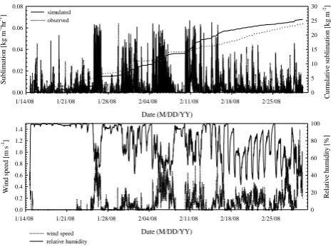
Fig. 5. Top: observed and simulated hourly (and cumulative) canopy snow sublimation; bottom: corresponding observations of forest wind speed and relative humidity.

is further investigated here. Evaluation of canopy sublima-tion was performed using canopy snowload measurements from a spruce tree suspended from a load cell at the Mar-mot Creek spruce forest site (Fig. 2). Changing tree weight was correlated to the intercepted snowload by the measured difference in snow accumulations between the forest and an adjacent clearing site (e.g. Hedstrom and Pomeroy, 1998). Decreases in tree tare from desiccation and needleleaf loss were accounted for, as was snow unloading from the canopy by measurements of snow collected in three lysimeters sus-pended under the canopy. Simulation of canopy sublimation was performed for the period of 14 January to 3 March using precipitation and incoming radiation data from the adjacent clearing with observations of within-canopy wind speed and humidity at the suspended tree.

Over the period, approximately one-half of snowfall was lost by canopy sublimation, with respective mean daily ob-served and simulated losses of 0.52 kg m−2and 0.55 kg m−2, giving a MB of 1.06 and a ME of 0.41. The time-series of hourly canopy sublimation losses in Fig. 5 (top) shows a gen-eral agreement between observed and simulated values, with

higher rates corresponding to periods of relatively high wind speeds and low relative humidity (Fig. 5, bottom). Overall, the cumulative amounts of observed and simulated sublima-tion were similar, equal to approximately 24 and 26 kg m−2 over the period, respectively.

4.3 Simulation of energy fluxes to snow

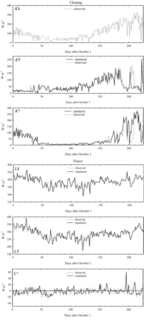
To investigate CRHM’s handling of energy fluxes, simula-tions of energy fluxes to snow were compared to measure-ments made at the Marmot Creek paired pine forest and clearing sites. Measurements from these sites include incom-ing and outgoincom-ing shortwave and longwave radiation, as well as ground heat fluxes. However, as no direct measures of sen-sible and latent heat were made, evaluation of the simulation of these fluxes was not possible.

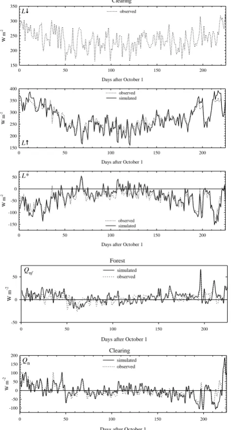
Time-series plots of observed and simulated energy terms during snowcover in Fig. 6 and model indices in Table 5 show a good agreement for all shortwave radiation terms at forest and clearing sites, and good prediction of net longwave radi-ation (L*) at the clearing site. However, even with the good prediction of the individual incoming and outgoing longwave fluxes (L↓and L↑) at the forest, the prediction of forest

L* was poor, which contributed to degrading estimates of total net radiation to forest snow (i.e.Qn=K*+L*). De-spite the large errors in estimating the ground energy flux (Qg)at the forest and clearing sites, little effect on overall model performance resulted due to the small contribution of

Qg to total energy (note that no energy to snow from rain-fall,Qp, was observed or simulated). In terms of systematic bias, the small negative and positive values ofL*,QnandQg observed (and simulated) provided MB values that were of-ten misleading and not instructive to model assessment. Al-ternatively, the systematic model bias of energy terms was evaluated simply as the difference between the mean of sim-ulated and observed values. Here, the offsetting of small neg-ative and positive biases of individual energy terms resulted in low bias errors of total energy to snow (Q*) at the forest and clearing sites of−0.59 and−0.37 W m−2, respectively. Furthermore, the close comparison of total simulated and ob-served energy terms in Fig. 7 demonstrate that CRHM was

[image:10.595.51.285.221.394.2]

(11)

K

0 50 100 150 200

0 20 40 60 80

simulated observed

0 50 100 150 200

0 10 20 30 40 50

simulated observed

0 50 100 150 200

W

m

-2

0 10 20 30 40 50

simulated observed Forest

K* K

W

m

-2

W

m

[image:11.595.50.284.66.321.2]

-2

Fig. 6. Time series plots of mean daily simulated and observed shortwave (K) and longwave (L) radiation fluxes, as well as total net radiation to snow (Qn) at pine forest and clearing sites at Mar-mot Creek, Alberta, Canada.

able to characterise the substantial difference between forest and clearing energy balances, and provide a good estimation of total energy to snow. Also shown in Fig. 7 are the simu-lated sensible and latent energy totals, which were greater in absolute magnitude at the clearing to that of the forest, but provided approximately equal contributions relative toQ* at both sites.

5 Discussion and conclusions

Overall, results show that CRHM is able to well represent the quantity and timing of snow accumulation and melt under needleleaf forest cover and in open forest clearings. Good results were obtained in terms of characterising the substan-tial differences in snow accumulation and melt observed in open and forest environments at locations of varying location and climate. The accurate representation of the major energy terms between the pine forest and clearing sites suggests that despite modest data requirements, the physical basis of the model is sufficient for representing forest-snow processes in environments of varying forest cover and meteorology.

Simulations of mean and maximum seasonal SWE exhib-ited little systematic bias at forest sites, clearing sites, or all sites. This suggests that much of the errors incurred were random in nature, resulting either from errors in observations or model parameterisation. For simulations of SWE at

indi-K

0 50 100 150 200

W

m

-2

0 100 200 300 400

observed

0 50 100 150 200

250 simulated

observed

0 50 100 150 200

W

m

-2

0 50 100 150 200 250 300

simulated observed Clearing

K* K

W

m

-2

Forest

0 50 100 150 200

W

m

-2

150 200 250 300 350 400

observed simulated

0 50 100 150 200

W

m

-2

150 200 250 300 350 400

L

observed simulated

0 50 100 150 200

W

m

-2

-40 -20 0 20 40 60

L

L* observed

[image:11.595.309.546.70.601.2]

simulated

(12)

Clearing

0 50 100 150 200

W m -2 150 200 250 300 350 observed

0 50 100 150 200

W m -2 150 200 250 300 350 400 L observed simulated

0 50 100 150 200

W m -2 -150 -100 -50 0 50 observed simulated L L*

Qnf

0 50 100 150 200

W m -2 -50 0 50 simulated observed Forest Q_n

0 50 100 150 200

W m -2 -100 -50 0 50 100 150 200 simulated observed Clearing Figure 6.

Fig. 6. Continued.

vidual sites, errors also appear to be random rather than sys-tematic, considering that the best and worst model efficien-cies were obtained for the same site over consecutive winters (i.e. Alptal forest). In all, the poorest model efficiencies of SWE determinations were realised at the 2003–2004 Alptal forest and Marmot pine sites, which had substantially lower accumulations relative to most other sites. Such results may be expected as shallower snowpacks would be more sensitive to simulation errors of mass and energy, thus giving larger relative errors. Notwithstanding these limitations, encourag-ing simulation results were obtained, as exemplified in the good representation of the extreme differences in forest and clearing snow accumulations observed over the two winters at the Alptal location.

Cleari ng (ob

serv ed) W m -2 -60 -40 -20 0 20 40 60 80 100 K* L* Qh Q_e Qg Cle aring (sim ulat ed) Cle aring (ob serv edQ* ) Cle aring (sim ulat edQ* ) Fores t (o bserv ed) Fores t (sim

ulat ed) Fores t (o bserv edQ* ) Fores t (sim

ulat edQ*

[image:12.595.317.537.64.257.2]

)

Figure 7. Fig. 7. Observed and simulated net energy terms and total energy

to snow (Q* = dU/dt+Qm)at pine forest and clearing sites (note that due to no observations of simulated sensible (Qh) and latent (Qe)heat fluxes, observations are assigned the same value as simu-lations).

Although good prediction of SWE was made for the start and peak of winter accumulations, poorer predictions were made at the end of accumulation, suggesting a lag in simu-lated melt rates. Particularly large lags in simusimu-lated snow de-pletion occured at the Alptal (2003–2004) clearing and Mar-mot spruce clearing sites, where the substantial late-season snowfall may have resulted in an overestimation of the addi-tional energy deficit to the snowpack. As such, improvement in CRHM’s representation of snowmelt timing and rate may require addressing the handling of internal snow energetics with large snowfalls.

Compared to observations of canopy snow load changes from a suspended tree, satisfactory model simulation of canopy sublimation was achieved both in terms of daily and cumulative losses. The correspondence of periods of high sublimation with relatively high wind speeds and low rel-ative humidity demonstrate the physically-based manner in which canopy sublimation is accounted for by CRHM. Ac-cordingly, such approaches are likely necessary to predict differences in snow accumulation between forest and clear-ings resulting from variations in forest cover density and cli-mate. However, sensitivity analysis has shown sublimation estimates in CRHM to be very responsive to errors in the intercepted snowload, which may have been brought about by the rather simplistic approach in the handling of canopy snow unloading by CRHM. Consequently, increased confi-dence in the model’s representation of canopy sublimation losses would likely by gained through a better understand-ing of the physical processes controllunderstand-ing canopy unloadunderstand-ing of snow.

[image:12.595.48.286.69.512.2]

(13)

[image:13.595.79.513.131.258.2]

Table 5. Model efficiency index (ME), root mean square error (RMSE), and the difference between mean simulated and observed values of: shortwave irradiance (K↓), reflected shortwave irradiance (K↑), net shortwave radiation (K∗), longwave irradiance (L↓), longwave exitance (L↑), net longwave radiation (L∗), total net radiation (Qn), net ground heat flux (Qg), and total energy to snow (Q∗)(i.e.Q* =Qm+ dU/dt ) for pine forest and clearing sites at Marmot Creek, Alberta, Canada.

Site: K↓ K↑ K∗ L↓ L↑ L∗ Qn Qg aQ∗

ME (Clearing) [] – 0.94 0.94 – 0.82 0.67 0.80 −0.92 0.78

ME (Forest) [] 0.87 0.82 0.83 0.90 0.79 0.08 0.27 −2.77 0.25

RMSE (Clearing) [W m−2] – 13.9 13.9 - 18.2 18.2 22.4 1.8 23.1

RMSE (Forest) [W m−2] 6.1 5.3 2.7 9.24 13.1 8.56 9.08 2.2 9.64

Mean simulated – mean observed – 2.75 −2.75 – −3.15 3.15 0.40 −0.03 −0.37 (Clearing) [W m−2]

Mean simulated – mean observed 0.36 −0.02 0.38 −2.70 −1.70 −1.0 −0.60 0.02 −0.59 (Forest) [W m−2]

a_{excludes sensible and latent heat fluxes}

Although simulations of energy fluxes were evaluated against observations at only a single paired forest and clear-ing site, results show the model able to well represent both the total energy to snow and the relative contributions of in-dividual energy terms. Furthermore, all errors in estimating shortwave and longwave radiation were small and below the measurement error of the radiometers used in their observa-tion. However, the presence of forest cover is seen to dra-matically decrease the model’s predictive capability of net radiation and total energy to snow, as seen in the decreas-ing model efficiency with the increasdecreas-ing number of com-bined energy terms. Yet, cumulative errors in estimating total energy to snow were relatively modest, owing in part to the error cancellation of individual energy terms. Al-though no evaluation of sensible and latent energy terms was possible, simulated magnitudes were similar to those observed in cold-region needleleaf forest environments by Harding and Pomeroy (1996) and estimated by Pomeroy and Granger (1997).

(14)

Appendix A

Notation

B fraction of ice in wet snow [] C Celsius [◦]

Cc fraction of horizontal canopy coverage []

Ce intercepted snow exposure coefficient []

Cl “canopy-leaf contact area” per unit ground []

cp specific heat capacity of air [J kg−1K−1]

CR canopy rain depth [mm]

E evaporation from a partially-wetted canopy [kg m−2t−1]

Ep evaporation from a fully-wetted canopy [kg m−2t−1]

ea vapour pressure [kPa]

eamean mean daily vapour pressure [kPa]

F exponent value []

h forest height [m]

Hin incoming horizontal snow transport rate [kg m−2t−1]

Hout outgoing horizontal snow transport rate [kg m−2t−1]

hr hour []

Ir canopy rainfall interception rate [kg m−2t−1]

Ir,o canopy intercepted rainload [kg m−2]

Is canopy snowfall interception rate [kg m−2t−1]

Is,o canopy intercepted snowload [kg m−2]

I*s species-specific maximum intercepted snowload [kg m−2]

k intercepted snow shape coefficient [] K degrees Kelvin []

K↓ shortwave irradiance [MJ m−2t−1or W m−2]

K↓_f sub-canopy shortwave irradiance [MJ m−2lt−1or W m−2_]

K↑ reflected shortwave irradiance [MJ m−2_t−1 _or W m−2]

K∗ net shortwave radiation [MJ m−2t−1or W m−2]

L↓ longwave irradiance [MJ m−2t−1or W m−2]

L↓_f sub-canopy longwave irradiance [MJ m−2t−1 or W m−2]

L↑ surface longwave exitance [MJ m−2t−1 or W m−2_]

L∗ net longwave radiation [MJ m−2_t−1_{or W m}−2_] LAI’ effective leaf area index []

M snowmelt rate [kg m−2_t−1_] MB model bias index [] ME model efficiency index []

n number []

P precipitation rate [kg m−2_t−1_]

Pr rainfall rate [kg m−2t−1]

Ps snowfall rate [kg m−2t−1]

qe canopy sublimation rate [kg m−2s−1]

Qe net latent heat flux [MJ m−2t−1or W m−2]

Qg net ground heat flux [MJ m−2t−1or W m−2]

Qh net sensible heat flux [MJ m−2t−1or W m−2]

Qm snowmelt energy [MJ m−2t−1or W m−2]

Qn total net radiation to snow [MJ m−2t−1or W m−2]

Qnf total net radiation to forest snow [MJ m−2t−1or W m−2]

Qp energy from rainfall advection [MJ m−2t−1or W m−2_]

Q* net energy to snow [MJ m−2_t−1_{or W m}−2_]

ra aerodynamic resistance [s m−1]

Rd canopy rain drip rate [kg m−2t−1] RH relative humidity [%]

RMSE root mean square error [units variable]

S sublimation loss rate [kg m−2t−1]

S mean maximum snowload per unit area of branch [kg m−2]

SWE snow water equivalent [kg m−2]

SWEo antecedent snow water equivalent [kg m−2]

t timestep [variable]

Ta air temperature [◦C or K]

Tb threshold ice-bulb temperature for snow unload-ing [◦_C]

Tf forest temperature [K]

Tmax maximum daily air temperature [◦C]

Tr rainfall temperature [◦C]

u wind speed [m s−1]

uh wind speed at canopy top [m s−1]

umean mean daily wind speed [m s−1]

uξ within-canopy wind speed at depthξfrom canopy top [m s−1_]

U internal (stored) snow energy [MJ m−2_t−1_]

Ul canopy snow unloading rate [kg m−2t−1]

Vi sublimation rate of intercepted snow [s−1]

Vs simulated sublimation flux for a 500µm radius ice-sphere [s−1]

xavg average observed value []

xobs observed value []

xsim simulated value []

αs snow albedo []

λf latent heat of fusion [MJ kg−1]

λs latent heat of sublimation [MJ kg−1]

1 slope of saturation vapour pressure curve [kPa K−1_]

εf thermal emissivity of forest cover []

εs thermal emissivity of snow []

θ solar elevation angle [radians]

ξ depth from canopy top (as a fraction of forest height) []

ρa density of air [kg m−3]

ρs density of snowfall [kg m−3]

ρw density of water [kg m−3]

σ Stefan-Boltzmann constant [W m−2_K−4_]

τ forest shortwave transmittance []

v sky view factor []

ψ canopy wind speed extinction coefficient []

wa specific mixing ratio of air []

ws saturation mixing ratio of air []

(15)

C. R. Ellis et al.: Simulation of forest snow accumulation and melt 939 Acknowledgements. The authors would like to thank R. Essery and

N. Rutter for their efforts in facilitating the SnoMIP2 initiative, which provided an invaluable opportunity for model evaluation and improvement. Funding and support was provided by the Natural Sciences and Engineering Research Council of Canada Alexander Graham Bell Doctoral and Michael Smith Foreign Stu-dent Supplement scholarships and Discovery Grants, the Canada Research Chairs Program, the Canadian Foundation for Climate and Atmospheric Science IP3 Network, Alberta Department of Sustainable Resource Development, the Canada Foundation for Innovation (CFI), the Natural Environment Research Council (UK), the GEWEX Americas Prediction Project (GAPP), and the Biogeosciences Institute, University of Calgary.

Edited by: W. Quinton

References

Anderson, E. A.: A point energy and mass balance model of a snow cover, NWS Technical Report 19, National Oceanic and Atmo-spheric Administration, Washington, DC, USA, 150 pp., 1976. Eagleson, P. S.: Ecohydrology, Darwinian expression of vegetation

form and function, Cambridge University Press, Cambridge, UK, 443 pp., 2002.

Ellis, C., Pomeroy, J., Essery, R., and Link, T.: Effects of needle-leaf forest cover on radiation to snow and snowmelt dynamics in the Canadian Rocky Mountains, Can. J. Forest Res., submitted, 2010.

Essery, R., Rutter, N., Pomeroy, J., Baxter, R., St¨ahli, R., Gustafs-son, D., Barr, A., Bartlett, P, and Elder, K.: An evaluation of forest snow process simulations, B. Am. Meteorol. Soc., 90(8), 1120–1135, 2009.

Essery, R. L. H., Pomeroy, J. W., Ellis, C., and Link, T.: Modelling longwave radiation to snow beneath forest canopies using hemi-spherical photography and linear regression, Hydrol. Process., 22, 2788–2800, doi:10.1002/hyp.6630, 2008.

Flerchinger, G. N. and Saxton, K. E.: Simultaneous heat and wa-ter model of a freezing snow-residue-soil system I. Theory and development, Trans. of ASAE, 32(2), 565–571, 1989.

Gelfan, A., Pomeroy, J. W., and Kuchment, L.: Modelling forest cover influences on snow accumulation, sublimation and melt, J. Hydrometeorol., 5, 785–803, 2004.

Gray, D. M. and Male, D. H. (Eds): Handbook of Snow: Princi-ples, Processes, Management and Use, Pergamon Press, Toronto, Canada, 776 pp., 1981.

Gray, D. M. and Landine, P. G.: An energy budget snowmelt model for the Canadian Prairies, Can. J. Earth Sci., 22(3), 464–472, 1988.

Gryning, S. and Batchvarova, E.: Energy balance of a sparse conif-erous high-latitude forest under winter conditions, Boundary Layer Meteorology, 99, 465–488, 2001.

Harding, R. J. and Pomeroy, J. W.: The energy balance of the winter boreal landscape, J. Climate, 9, 2778–2787, 1996.

Hardy, J. P., Melloh, R., Robinson, P., and Jordan, R.: Incorporating effects of forest litter in a snow process model, Hydrol. Process., 14, 3227–3237, 2000.

Hardy, J., Melloh, R., Koenig, G., Marks, D., Winstral, A., Pomeroy, J. and Link, T.: Shortwave radiation transmission

through conifer canopies, Agr. Forest. Meteorol., 126, 257–270, 2004.

Hedstrom, N. R. and Pomeroy, J. W.: Measurements and modelling of snow interception in the boreal forest, Hydrol. Process., 12, 1611–1625, 1998.

Hellstr¨om, R. ˚A.: Forest cover algorithms for estimating meteo-rological forcing in a numerical snow model, Hydrol. Process., Special Issue: Eastern Snow Conference, 14(18), 3239–3256, 2000.

Jordan, R.: Special Report 91–16, A one-dimensional temper-ature model for a snow cover, Technical documentation for SNTHERM.89. US Army Corps of Engineers Cold Regions Re-search and Engineering Laboratory, Hanover, New Hampshire, 49 pp., 1991.

Koivusalo, H. and Kokkonen, T.: Snow processes in a forest clear-ing and in a coniferous forest, J. Hydrol., 262, 145–164, 2002. Link, T. E. and Marks, D.: Point simulation of seasonal snow cover

dynamics beneath boreal forest canopies, J. Geophys. Res., 104, 27841–27857, 1999.

Link, T. E., Marks, D., and Hardy, J.: A deterministic method to characterize canopy radiative transfer properties. Hydrol. Pro-cess., 18, 3583–3594, 2004.

Lundberg, A. and Halldin, S.: Evaporation of intercepted snow, analysis of governing factors, Water Resour. Res., 30, 2587– 2598, 1994.

Marks, D., Domingo, J., Susong, D., Link, T., and Garen, D.: A spa-tially distributed energy balance snowmelt model for application in mountain basins, Hydrol. Process., 13, 1935–1959, 1999. McNay, R. S., Petersen, L. D., and Nyberg, J.B.: The influence of

forest stand characteristics on snow interception in the coastal forests of British Columbiam, Can. J. Forest Res., 18, 566–573, 1988.

Melloh, R. A., Hardy, J. P., Bailey, R. N., and Hall, T. J.: An effi-cient snow albedo model for the open and sub-canopy, Hydrol. Process., 16, 3571–3584, 2002.

Metcalfe, R. A. and Buttle, J. M.: Controls of canopy structure on snowmelt rates in the boreal forest, Proceedings of the 52nd East-ern Snow Conference, 249–257, 1995.

Monteith, J. L.: Evaporation and environment, Sym. Soc. Exp. Biol., 19, 205–234, 1965.

Parviainen, J. and Pomeroy, J. W.: Multiple-scale modelling of forest snow sublimation, initial findings, Hydrol. Process., 14, 2669–2681, 2000.

Pomeroy, J. W. and Schmidt, R. A.: The Use of Fractal Geometry in Modelling Intercepted Snow Accumulation and Sublimation, Proceedings of the Eastern Snow Conference, 50, 1–10, 1993. Pomeroy, J. W. and Gray, D. M.: Snowcover Accumulation,

Relo-cation and Management, NHRI Science Report No. 7, National Hydrology Research Institute, Environment Canada, Saskatoon, SK, 134 pp., 1995.

Pomeroy., J. W. and Dion, K.: Winter radiation extinction and re-flection in a boreal pine canopy, measurements and modelling, Hydrol. Process., 10, 1591–1608, 1996.

(16)

940 C. R. Ellis et al.: Simulation of forest snow accumulation and melt 1997.

Pomeroy, J. W., Parviainen, J., Hedstrom, N., and Gray, D. M.: Coupled modelling of forest snow interception and sublimation, Hydrol. Process., 12, 2317–2337, 1998a.

Pomeroy, J. W., Gray, D. M., Hedstrom, N. R., and Janowicz, J. R.: Prediction of seasonal snow accumulation in cold climate forests, Hydrol. Process., 16, 3543–3558, 2002.

Pomeroy, J. W., Gray, D. M., Brown, T., Hedstrom, N. R., Quinton, W. L., Granger, R. J., and Carey, S. K.: The cold regions hydro-logical model, a platform for basing process representation and model structure on physical evidence, Hydrol. Process., 21(20), 2650–2667, 2007.

Pomeroy, J. W., Marks, D., Link, T., Ellis, C., Hardy, J., Rowlands, A., and Granger, R.: The impact of coniferous forest tempera-ture on incoming longwave radiation to melting snow, Hydrol. Process., 23(17), 2513–2525, doi:10.1002/hyp.7325, 2009. Rutter, N., Essery, R., Pomeroy, J., Altimir, N., Andreadis, K.,

Baker, I., Barr, A., Bartlett, P., Boone, A., Deng, H., Douville, H., Dutra, E., Elder, K., Ellis, C., Feng, X., Gelfan, A., Good-body, A., Gusev, Y., Gustafsson, D., Hellstrom, R., Hirabayashi, Y., Hirota, T., Jonas, T., Koren, V., Kuragina, A., Lettenmaier, D., Li, W-P, Martin, E., Nasanova, O., Pumpanen, J., Pyles, R., Samuelsson, P., Sandells, M., Schadler, G., Shmakin, A., Smirnova, T., Stahli, M., Stockli, R., Strasser, U., Su, H., Suzuki, K., Takata, K., Tanaka, K., Thompson, E., Vesala, T., Viterbo, P., Wiltshire, A., Xia, K., Xue, Y., and Yamazaki, T.: Evaluation of forest snow process models (SnowMip2), J. Geophys. Res.-Atmos., 114, D06111, doi:10.1029/2008JD011063, 2009.

Rutter, A. J., Kershaw, K. A., Robins, P. C., Morton, A. J.: A pre-dictive model of rainfall interception in forests. I. Derivation of the model from observations in a plantation of Corsian pine, Agr. Meteorol., 9, 367–384, 1971.

Schmidt, R. A., Jairell, R. L., and Pomeroy, J. W.: Measuring snow interception and loss from an artificial conifer, P. West. Snow Conf., 56, 166–169, 1988.

Schmidt, R. A.: Sublimation of snow by an artificial conifer, Agr. Forest Meteorol., 54, 1–27, 1991.

Sicart, J. E., Pomeroy, J. W., Essery, R. L. H., Hardy, J. E., Link, T., and Marks, D.: A sensitivity study of daytime net radiation during snowmelt to forest canopy and atmospheric conditions, J. Hydrometeorol., 5, 744–784, 2004.

Troendle, C. A. and King, R. M.: The effect of timber harvest on the Fool Creek watershed: 30 years later, Water Resour. Res., 21, 1915–1922, 1985.

Valente, F., David, J. S. and Gash, J. H. C.: Modelling interception loss for two sparse eucalypt and pine forests in central Portugal using reformulated Rutter and Gash analytical models, J. Hy-drol., 190, 141–162, 1997.