Munich Personal RePEc Archive
Inflation and consumption in a long term
perspective with level shift
Casadio, Paolo and Paradiso, Antonio
University of Rome La Sapienza
11 September 2010
Online at
https://mpra.ub.uni-muenchen.de/25980/
Inflation and consumption in a long term perspective with level shift
Paolo Casadio
†and Antonio Paradiso
† Intesa Sanpaolo Bank, Risk Management.
ISAE (Institute for Studies and Economic Analysis) and Univeristy of Rome La Sapienza; e-mail: [email protected]; [email protected].
This article examines the existence and stability of the consumption function in the United States of America (US) economy during a sample period, beginning in the 1950s. In order to obtain a stable long run relationship, we have introduced two innovative elements into the analysis of the life-cycle of the consumption function with wealth effects: 1) a shift level break in the cointegrating relationship, and 2) using inflation as an additional explanatory variable. By implementing a well structured estimation strategy we found that, after taking the shift level break into account, a cointegration including inflation exists and is more stable for the critical sub-samples than traditional consumption function models.
I.
INTRODUCTION
The aim of this paper is to study the personal consumption expenditure (PCE) in the US over a period spanning more than 50 years. Traditionally, the consumption dynamic has been studied according to the framework of the life-cycle model (LCM) of household behaviour, in which wealth and income determine consumer spending. The most commonly used technique for analysis is the cointegration method. The problem with this technique is that cointegration models implicitly require the existence of a stable long term relationship between consumption, income and wealth. The 50 year span of the available data comprises major changes in taxes, demographics, productivity growth, financial structure, social insurance, and every other aspect of reality incorporated into the theory (and then embodied in the cointegrating vector (Carroll et al., 2006)). We, therefore, agree with Carroll et al. (2006) that trying to find the existence of a cointegrating relationship which satisfies the condition of stability is a very problematic process. Bearing in mind Carroll et al.’s (2006) criticism regarding the stability of a long run relationship, we checked for the existence and stability of a cointegrating relationship involving consumption, income and wealth in various forms. In particular, in order to determine the level of stability, we introduced two innovative elements into the analysis: 1) the possibility that a shift level break in the long term relationship has occurred in the last 10 years due to the presence of various shocks, and 2) we allowed for consumer price index (CPI) inflation as an additional explanatory variable in the consumption function. Whether or not a level break was present in the constant was checked statistically. The hypothesis regarding an adjustment in the constant, leaving the coefficient unchanged, is simple and not invasive, as it introduces minimal change in the statistical relationship. CPI inflation exerts an influence on consumption in several ways. The simplest is that inflation adversely affects consumer confidence and thus leads to increased saving. Inflation may also change the distribution of income among households and affect consumer behavior in that way. However, most importantly, inflation can be linked to the cash-out mechanism which began to operate in the beginning of the 1990s.
II.
LITERATURE REVIEW
The LCM of Ando and Modigliani (1963) is the basic theoretical framework for studying the effect of income and total wealth on consumer spending, as well the earliest empirical work1 on the subject. They studied the relationship between consumption, labour income and total wealth.
In the last 10 years, stimulated by the sharp increase in equity markets and by the development of cointegration analysis, a growing number of empirical studies have focused on the link between stock market wealth and consumption. Ludvigson and Steindel (1999), in an influential paper, employed a traditional LCM that links consumption, labour income and asset wealth, focusing on the wealth effects due to the stock market during the stock market boom of the late 1990s. The researchers found a significant cointegrating relationship between consumption, income and wealth. They also noted that the long run relationship between these variables was not very stable.
Many papers on LCM have found a statistically significant cointegrating relationship between consumption, labour income and wealth measures. A study by Rudd and Whelan (2002, 2006) raised some questions about these works. They stated that there was an inconsistency, due to the underlying budget constraints, in the measures of real consumption, income and wealth that were used.2 They concluded that, with proper measures of consumption, income and wealth, there would be cointegration. A recent study by Donihue and Avramenko (2006) looked for a cointegrating relationship between consumption (including durable goods), labour income and different forms of wealth over a wide sample period (spanning from 1952 to 20063). This study showed that there is no cointegration if the criteria for significance are not extended to over 10% of the critical values.
Carroll (2006), due to a range of empirical and theoretical problems, was skeptical about the possibility of finding a stable cointegration relationship spanning from the 1950s until now. The author cites some problems inducing a structural break affecting the behavior of consumers (demographic factors as well as the institutional transformation of the financial system are examples of factor inducing breaks) that make it very difficult to find a stable long run relationship.
Other studies have tried to identify other variables that, in addition to income and wealth, may affect consumer expenditure. In the 1970s and 1980s, serious attempts were made to estimate the effect of nominal interest rates and inflation on aggregate consumption and saving in the US. Taylor (1971) and Heien (1972) measured interest rates in nominal terms and reported empirical evidence of an inverse relationship between consumption and interest rates. Similar results were found by Mishkin (1976), Gylfason (1981) and Wilcox (1985). Contradictory results have been presented by Weber (1975) and Springer (1975). Springer (1977) also found that the effects of nominal interest rates and inflation are different for different components of aggregate consumption and for different measures of predicted inflation. Howard (1978) has reported evidence of a positive relationship between inflation and saving in the US, but he found no evidence of the effects of interest rates. The fact that, during this period, these studies focused on inflation is not coincidental. The dynamic increase in prices made the effect of inflation
1
Earlier empirical studies are based on regression analysis, not taking into account the possibility that the variables show non stationary patterns. This problem could lead to inconsistent estimates.
2 The problem raised by Rudd and Whelan (2002, 2006) is as follows. Much of the earlier consumption literature
focuses on the consumption of non durables. One justification for this is that these studies test for a behavioural relationship based on the utility derived from the flow of consumption. This utility function maximisation applies to goods and services providing utility in the current period and expiring after one period. Durable goods persist for several periods, and this does not fit with the theoretical hypothesis of the consumption function. To include durable goods in the consumption function, in accordance with the utility function approach, it is necessary to consider the flow of services coming from the consumption of durable goods. Even this alternative presents some problems, since the flow of services from durable goods is difficult to measure and implies some discretional evaluations about depreciation rate. For these reasons, durable goods are usually omitted from aggregate consumption measures. With a properly constructed budget constraint - that is, total consumption expenditures and asset measures which exclude the value of the stock of consumer durables - they found no cointegration with the traditional consumption function.
3
on consumption evident. When inflation returned to normal patterns, the amount of attention paid to the impact of inflation on consumption rapidly declined.
A more recent strand of literature considers the role of mortgage equity withdrawal (MEW) in explaining consumption expenditure together with the variables traditionally included in the LCM (that is, net wealth and labour income). Fuentes and Hatzius (2006) focused on the effect of MEW on consumption and found a statistically significant positive coefficient of MEW in the consumption equation. Prakken (2007) analysed Fuentes and Hatzius’ (2006) results and demonstrated that their estimation suffered from some econometric problems: first, the authors did not examine the long run relationship; second, the residual ADF test for a cointegrating relationship is non stationary.
Another field of interest is the study of asymmetries in consumer wealth effects, particularly for the period following the stock market bubble and the recent developments in the housing market. Apergis and Miller (2004) found that positive shocks to the stock market wealth affected consumption more than negative shocks. MacDonald et al. (2009) examined the possibility of asymmetry in the consumption wealth channel of monetary transmission for the United Kingdom (UK) economy. The authors concluded that changes in the interest rate inversely affect asset value which may have an asymmetric effect on consumption: wealth reduction due to monetary tightening has a weaker impact on spending than an increase in wealth.
III.
THE INFLATION RATE AND CONSUMPTION
The effects of income and wealth on consumption are well known from a theoretical perspective. A less frequently debated aspect in the literature, from a theoretical point of view, is the effects of inflation on consumer expenditure.
A number of attempts to explain the phenomenon of rising saving rates in the presence of high inflation have drawn upon the work of Katona (1975). Katona maintained that inflation causes uncertainty and pessimism about the future, pushing consumers to save more. Another direct effect of inflation upon consumption is due to the incentive of holding real assets rather than assets fixed to nominal values. In this regard, inflation affects liquid and illiquid assets in different ways.
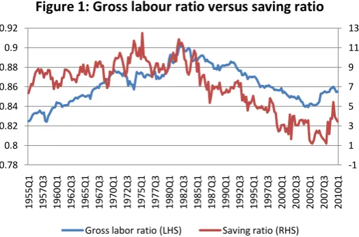
Figure 1: Gross labour ratio versus saving ratio -1 1 3 5 7 9 11 13 0.78 0.8 0.82 0.84 0.86 0.88 0.9 0.92 1 9 5 5 Q 1 1 9 5 7 Q 3 1 9 6 0 Q 1 1 9 6 2 Q 3 1 9 6 5 Q 1 1 9 6 7 Q 3 1 9 7 0 Q 1 1 9 7 2 Q 3 1 9 7 5 Q 1 1 9 7 7 Q 3 1 9 8 0 Q 1 1 9 8 2 Q 3 1 9 8 5 Q 1 1 9 8 7 Q 3 1 9 9 0 Q 1 1 9 9 2 Q 3 1 9 9 5 Q 1 1 9 9 7 Q 3 2 0 0 0 Q 1 2 0 0 2 Q 3 2 0 0 5 Q 1 2 0 0 7 Q 3 2 0 1 0 Q 1
Gross labor ratio (LHS) Saving ratio (RHS)
Note: Gross labour ratio = wages and salary disbursements/(wages and salary disbursements + proprietors’ income). Source: NIPA.
Inflation may also be linked to the cash-out mechanism, which operated mainly at the beginning of the 1990s, due to the fact that inflation is the main determinant of the nominal interest rate. The cash-out mechanism is the effect coming from interest payment saved due to a falls in interest rates. There are two main cash-out phenomena. The first one is the withdrawal of equity secured on a house (the effect known as mortgage equity withdrawal (MEW)) in the presence of a long term interest rate reduction. The second one is a more general mechanism, according to which a reduction in interest payments frees more resources that can be devoted to consumption.
One of the most commonly known facts about the monetary economy is that high inflation is associated with high nominal interest rates. This allows us to concentrate on the role of interest rates in the cash-out mechanism, knowing that a similar informational content is embodied in the inflation series.
As the second cash-out effect is very intuitive (and does not require in-depth study), we will focus on the MEW effect. Home equity can be extracted if either of the following two events occurs: 1) the value of the house increases, or 2) the current mortgage rate goes below the historically contracted one. In such cases the mortgage can be renegotiated, by increasing the loan amount or decreasing the service of debt, and thus freeing resources. The meaningful variable regarding mortgage cash-out is the nominal mortgage rate because mortgage debt is contracted in nominal terms, such as the payments owed.
Active MEW4 (AMEW) can thus be explained by means of a relationship involving the annual change in real house prices and the nominal fixed long term mortgage rate. A DOLS (dynamic OLS) estimation of this relationship is presented in Table 1.
Table 1: DOLS estimates of active MEW
Model amewt =
tk k J h j t j k k j mtg j t j h t mtg
t p i p
i
1, 2, 4
4 2 1 0
Long term relation amewt = 01itmtg24pthut
Sample Period β0 β1 β2
1991q1 – 2008q2 0.696 -0.389*** 0.209***
Residual ADF t- test -4.09**
4
[image:5.595.49.542.641.688.2]Note: *, ** and *** represent, respectively, significance levels of 10%, 5% and 1%. amew indicates the natural logarithm of active MEW. Leads and lags of DOLS estimations were selected according to HQ criteria. The sample period denotes the range of data before data points for leads and lags are removed. For the residual ADF t-test, the lag length was chosen by HQ criteria. Newey-West corrected t-statistics were applied in regression.
Our view of the MEW mechanism has been empirically confirmed by the results in Table 1. Since the dynamic of house prices has already been captured by the wealth component, the only component of the MEW mechanism not captured in the consumption estimation is the nominal long term interest rate. From the link between inflation and the nominal interest rates, we can conclude that inflation within the consumption function can carry information about cash-out.
Even if inflation and nominal interest rates are positively correlated, there will be an additional informational component not properly captured by inflation. Changes in interest rates can explain consumption in the short term. We will investigate whether a short term component can provide useful information in terms of consumption expenditure. Given the nature of the cash-out effect, we will question whether consumption responds asymmetrically to changes in interest rates. We expect to find strong evidence that a reduction in interest rates increases consumption.
IV.
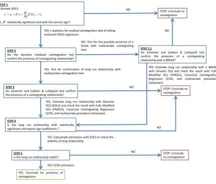
METHODOLOGY
The main aim of this empirical analysis is to compare various specifications of two consumption function formulations in order to find a stable cointegrating relationship: the traditional LCM and a version “augmented” for inflation. Following the most recent empirical literature on this topic, we considered the total net wealth as well as the various divisions of net wealth: stock versus non stock market wealth; housing versus non housing wealth, and liquid versus illiquid wealth. We also analysed the same disaggregation where the first components of wealth (stock, housing and liquid) were measured as an asset (excluding liability components) and the residual wealth was calculated as the difference between the total net wealth and the asset under consideration. Details of the data construction and sources are reported in the appendices.
Figure 2: The decision-making strategy adopted in the empirical estimation
STEP 1 Estimate DOLS
Is statistically significant and with the correct sign?
k
k i
t i t i t o
t a x x
c ' ' STOP: Conclude no
cointegration
YES: t-statistics for residual cointegration test of rolling end point DOLS regression.
STEP 2
Do the dynamic residuals cointegration test confirm the presence of cointegrating relationship?
YES: Test for confirmation of long run relationship with multivariate cointegration test.
STEP 3
Do Johansen and Saikkon & Lutkepohl test confirm the presence of a cointegrating relationship?
STOP: Conclude no cointegration
YES: Estimate long run relationship with Dynamic OLS (DOLS) and check the result with Fully Modified OLS (FMOLS), Canonical Cointegrating Regression (CCR), and multivariate procedure (Johansen).
STEP 4
Is the long run relationship with statistically significant and expect sign coefficients ?
YES: Subsample estimation with DOLS to check the stability of long relationship
STEP 5
Is the long run relationship stable?
STOP: Conclude no cointegration
YES: ECM estimation
YES: Conclude for presence of cointegration
NO: Test for the possible presence of a break with multivariate cointegrating
test. STEP 2.1
Do Johansen and Saikkon & Lutkepohl test confirm the presence of a cointegrating relationship with a BREAK?
NO NO
YES: Estimate long run relationship with a BREAK with Dinamic OLS and check the result with Fully Modified OLS (FMOLS), Canonical Cointegrating Regression (CCR), and multivariate procedure (Johansen).
NO
NO
NO
'
Source: Our elaboration.
The logic is simple: if an equation specification does not provide the required proof, then it is excluded from the successive steps and we can conclude that the variables in the equation are not cointegrated.
The starting point was the DOLS estimation technique devised by Stock and Watson (1993). After having verified that a model has statistically significant coefficients with the expected signs (STEP 1), we passed through the following steps. An ADF residual test was conducted on the residuals of a long run relationship estimated using DOLS. If the residuals were stationary, then additional (multivariate) tests (the Johansen trace test and the Saikkonen and Lutkepohl test (STEP 3)) were conducted in order to confirm the presence of a cointegrating relationship. However, if, as we expected following the conclusions of Section I, the residuals appear to be non stationary, additional analysis is required. We checked, from a visual inspection of the residuals’ t-statistics5, whether a structural break had occurred. If this was the case, we could pass on to STEP 2.1 in order to confirm the presence of a cointegrating relationship with the shift level on constant through the Johansen trace test and the Saikkonen and Lutkepohl multivariate tests (the results of this step are reported in Table A in the appendices). The break in the constant causes minimal change to the statistical relationship. The subsequent step, STEP 4, aims to specify the cointegrating relationship through studying the signs and the statistical significance of the parameters entering into the long term relationship. We adopted three methods of estimation: DOLS, FMLS (fully modified OLS), CCR (canonical cointegrating regression), and the Johansen-maximum likelihood estimation (MLE). A restricted version of the VAR was employed alongside the Johansen-MLE procedure (a model that excludes from the ECM the factor loading
5
of the other explanatory variables). The last step (STEP 5) entailed studying the stability of the “surviving” models following all the previous steps. A visual description of this is depicted in Figure 3, which plots the savings ratio against the ratio of household net worth to disposable income.
Figure 3: Wealth-to-disposable-income ratio and personal saving rate
2.5 3.0 3.5 4.0 4.5 5.0 5.5 6.0 6.5 0
2 4 6 8 10 12 14
1
9
5
5
Q
1
1
9
5
7
Q
3
1
9
6
0
Q
1
1
9
6
2
Q
3
1
9
6
5
Q
1
1
9
6
7
Q
3
1
9
7
0
Q
1
1
9
7
2
Q
3
1
9
7
5
Q
1
1
9
7
7
Q
3
1
9
8
0
Q
1
1
9
8
2
Q
3
1
9
8
5
Q
1
1
9
8
7
Q
3
1
9
9
0
Q
1
1
9
9
2
Q
3
1
9
9
5
Q
1
1
9
9
7
Q
3
2
0
0
0
Q
1
2
0
0
2
Q
3
2
0
0
5
Q
1
2
0
0
7
Q
3
2
0
1
0
Q
1
Saving Ratio (LHS) TNW income ratio (RHS; reverse scale)
Source: U.S. Department of Commerce, Bureau of Economic Analysis; Board of Governors of the Federal Reserve System.
From a visual inspection of Figure 3 we selected the events which clearly influenced the pattern of this relationship. Until the 1980s, the personal saving rate increased while the wealth-to-disposable-income-ratio plunged. These trends inverted after the beginning of the 1980s, when there was a change in the slope of both the saving rate and total net wealth ratio. Since the beginning of the 1990s, the wealth-saving relationship has “relaxed”: the saving rate declined very steeply whereas the wealth ratio showed a less conclusive pattern. A view put forward by some authors (e.g. MacDonald et al., 2006) and practitioners is that the rapid increase in the conversion of homeowners equity to cash through borrowing in the home mortgage market (a phenomenon known as MEW) caused the rapid decline in the saving rate during the 1990s. The last 10 years appear to be the most problematic in terms of this relationship: the saving rate is characterised by its strong volatility and the net wealth ratio features accentuated peaks and troughs. This dynamic is due to numerous events that affected the US economy during this period (e.g. the rise and fall in the stock market, the housing market bubble and the financial crisis).
Bearing in mind that stability is a difficult condition to satisfy in a consumption estimation spanning from the 1950s to the present day, we divided the sample period into three subsamples: 1955q1 – 1980q1; 1980q1 – 2010q1; 1991q1 – 2010q1. This choice, as mentioned above, is not arbitrary: during the early years of the 1980s, the slopes of the saving rate and total-wealth-to-income ratio changed (and inflation started falling, after the second oil shock). The early years of the 1990s were when nominal interest rates became fairly volatile and the MEW mechanism (cash-out effect) exerted its strongest influence on consumption.
V.
ESTIMATION RESULTS
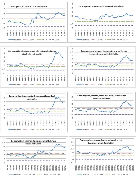
All the statistical results, on a step by step basis, are reported in Table 2. In Figure 4, the values of the residual ADF test coming from the DOLS estimations conducted in STEP 1 (dynamically extending the sample one quarter at a time) are illustrated, and we compared these values with the critical levels in order to asses if the stationary condition is satisfied. In the appendices (Table A), the results of the cointegration tests in STEP 2.1 are presented.
(Equation 4), and consumption-labour income-stock market asset-residual net wealth (Equation 6)6. The final two models appear to be almost identical, as we can see by comparing the results of various steps and looking at the coefficients that have been estimated. Therefore, we can consider these two equations as comprising only one result. This is because it makes no substantial difference whether we compute stock market values based on just on asset, or if we consider net wealth.
Between the two “surviving” formulations of the consumption function, Equations 1 and 4 (or 6), the latter is generally preferable, for empirical and theoretical reasons. As far as the empirical aspect is concerned, we can see that Equation 4 (or 6) is stable over a longer period of time (see Figure 4 of the ADF residual tests) before a break occurs in the relationship and it fits better the consumption.7 The most important aspect in empirical terms is the comparison of the estimates of the equations of the subsamples. Equation 1, which refers to the total net wealth, shows the regression coefficients relative to labour income in the subsamples. The estimates are all significantly higher than the levels estimated for the whole sample (with an approximate range of 0.85 – 0.92 in the subsamples, compared to a value of 0.70 over the whole period). This strange behaviour of the coefficients is offset by the analogous behavior of the net wealth coefficients of the subsamples, which are always lower than the coefficients obtained for the entire period (with an approximate range of 0.10 – 0.24 for the subsamples compared 0.36 value over the entire period). If we add the values of the labour income and net wealth coefficients, this results in a fairly stable value of approximately 1.05, independent of the period of time in which we estimated the consumption function. That means that a sort of compensation occurs between labour income and net wealth contribution to consumption. This suggests that the two effects are not entirely separate, and that they interfere with each other. This problem does not occur with Equations 4 or 6, where each coefficient over the whole sample can be seen as an average of the values of the coefficient over the subsamples. In the last case, only the variability of wealth components are high, especially with regard to the subsample 1991-2010, showing a significantly lower value for non stock coefficient.8 From a theoretical point of view, a more complex specification capable of the successful interpretation of the evolution of the main components of wealth would be preferable. Recent experience indicates a significantly different evolution of the stock market and of the housing market, a trend which seems set to continue in the future. In this case it is very important, in our opinion, to have a more detailed estimation of the consumption function which is able to quantify the individual contributions of the main components of wealth and not only the average effect of the total amount of wealth on consumption.9
After having identified the best equation, we investigated the presence of an asymmetrical short term effect of the nominal interest rate on consumption. This approach involved the estimation of ECM (with the error term of the long term relationship represented by Equation 410) with asymmetrical short term dynamics of the interest rate. The results of our estimation are shown in Table 3. As we expected, the magnitude of the effect of a negative change in the nominal interest rate (D- Δi) is twice that of a positive change (D+ Δi). In addition, a positive change is not statistically significant, confirming our view that the cash-out effect explicates its effect when interest rates decrease.
6 Equations 2, 8, 12 and 14 did not pass the first two steps, showing no cointegration. Equations 7, 11 and 13 show a
factor loading (in the Johansen-MLE procedure estimation) which is not statistically significant or incorrect in terms of the sign. Equations 3, 5, 9 and 10, which show a cointegrating relationship over the whole sample, do not pass the stability test for the coefficient signs over the three subsamples.
7
It is sufficient to compare the sum squared of error (SSE) of the two equations, obtaining a value of 0.02 for the inflation-augmented-disaggregated-wealth specification versus 0.05 for the simple aggregated wealth specification.
8
The stock market wealth coefficient, over the subsample 195-1980, is at the limit for statistical significance with a p-value of 0.11. This does not make a dent in the result because Equation 6 shows a significant p-value for this variable in the same subsample.
9
The marginal propensity to consume (relative to Model 4) out of the two wealth components and income are as follows: mpcINC = 0.982, mpcSW = 0.029, mpcNSW = 0.071. These values are in line with other empirical studies
conducted on the consumption function.
10
Table 2: Estimation results
STEP 1 STEP 2 STEP 2.1 STEP 4 (Sample 1955q1 – 2010q1) STEP 5
DOLS estimation
Cointegration dynamic Test
Cointegration + shift dummy
Cointegration different methods Subsamples comparison
1955q1 – 2010q1
DOLS CCR FMOLS VAR-MLE VAR-MLE
Restr.
1955q1 – 1980q1
1980q1 – 2010q1
1991q1 – 2010q1 EQUATION 1
Income 0.753*** NO YES 0.697*** 0.67*** 0.662*** 0.533*** 0.6*** 0.844*** 0.918*** 0.847*** TW 0.284*** (Fig. 4) (Table A) 0.355*** 0.379*** 0.388*** 0.499*** 0.451*** 0.103** 0.237*** 0.155***
Shift(97q4) - -0.036*** -0.04** -0.041*** -0.064*** -0.058*** - -0.052*** -
Factor load. - - - - -0.039*** -0.007 - - -
EQUATION 2
Income 0.925*** NO NO
TW 0.141*** (Fig. 4) (Table A) Inflation -0.007***
EQUATION 3
Income 0.692*** NO YES 0.621*** 0.663*** 0.656*** 0.535*** 0.481*** 0.591*** 0.91*** 0.992*** SW 0.047*** (Fig. 4) (Table A) 0.055*** 0.057*** 0.057*** 0.077*** 0.06*** 0.028*** 0.045*** 0.063*** NSW 0.298*** 0.368*** 0.332*** 0.337*** 0.415*** 0.489*** 0.392*** 0.146*** -0.039***
Shift(04q1) - -0.042*** -0.037*** -0.038*** -0.045*** -0.039*** - -0.031** -
Factor load. - - - - -0.053*** -0.029† - - -
EQUATION 4
Income 0.841*** NO YES 0.771*** 0.724*** 0.717*** 0.871*** 0.785*** 0.682*** 0.785*** 0.864*** SW 0.018** (Fig. 4) (Table A) 0.028*** 0.034*** 0.034*** 0.029*** 0.028*** 0.016† 0.052*** 0.064*** NSW 0.205*** 0.268*** 0.307*** 0.313*** 0.177*** 0.255*** 0.347*** 0.152*** 0.043** Inflation -0.006*** -0.005*** -0.004*** -0.004*** -0.008*** -0.007*** -0.004*** -0.007*** -0.003**
Shift(04q1) - -0.033*** -0.035*** -0.035*** -0.034*** -0.03*** - -0.015** -
Factor load. - - - - -0.136*** -0.126*** - - -
EQUATION 5
Income 0.688*** NO YES 0.623*** 0.665*** 0.66*** 0.543*** 0.491*** 0.595*** 0.906*** 0.979*** SA 0.055*** (Fig. 4) (Table A) 0.063*** 0.064*** 0.064*** 0.086*** 0.071*** 0.036*** 0.049*** 0.065*** RWS 0.296*** 0.36*** 0.324*** 0.329*** 0.402*** 0.472*** 0.384*** 0.144*** -0.034*
Shift(04q1) - -0.042*** -0.037*** -0.037*** -0.045*** -0.04*** - -0.031** -
Factor load. - - - - -0.054*** -0.032† - - -
Income 0.845*** NO YES 0.773*** 0.726*** 0.718*** 0.829*** 0.764*** 0.693*** 0.781*** 0.853*** SA 0.022*** (Fig. 4) (Table A) 0.034*** 0.041*** 0.041*** 0.038*** 0.036*** 0.022** 0.057*** 0.067*** RWS 0.199*** 0.263*** 0.3*** 0.307*** 0.207*** 0.267*** 0.331*** 0.149*** 0.046*
Inflation -0.006*** -0.005*** -0.004*** -0.004*** -0.007*** -0.006*** -0.003*** -0.007*** -0.003*
Shift(04q1) - -0.034*** -0.035*** -0.035*** -0.035*** -0.031*** - -0.015** -
Factor load. - - - - -0.136*** -0.117*** - - -
EQUATION 7
Income 0.733*** NO YES 0.63*** 0.691*** 0.721*** 0.414*** 0.345*** HW 0.095** (Fig. 4) (Table A) 0.161*** 0.097*** 0.101*** 0.277*** 0.319*** NHW 0.206*** 0.252*** 0.256*** 0.2229*** 0.34*** 0.364***
Shift(00q1) - -0.039*** -0.024† -0.029** -0.068*** -0.008***
Factor load. - - - - 0.009 0.002
EQUATION 8
Income 0.901*** NO NO
HW 0.063** (Fig. 4) (Table A) NHW 0.099***
Inflation -0.007***
Shift(00q1) -
Factor load. -
EQUATION 9
Income 0.736*** NO YES 0.638*** 0.658*** 0.633*** 0.529*** 0.503*** 0.68*** 1.11*** 1.11*** HA 0.132*** (Fig. 4) (Table A) 0.21*** 0.189*** 0.208*** 0.226*** 0.309*** 0.209*** 0.092*** -0.078***
RWH 0.159*** 0.168*** 0.171*** 0.172*** 0.243*** 0.178*** 0.052* 0.036 0.095***
Shift(02q1) - -0.038*** -0.051*** -0.054*** -0.05*** -0.057*** - -0.062*** -
Factor load. - - - - -0.054*** -0.044*** - - -
EQUATION 10
Income 0.895*** NO YES 0.802*** 0.739*** 0.746*** 0.772*** 0.82*** 0.754*** 0.918*** 0.96*** HA 0.078** (Fig. 4) (Table A) 0.157*** 0.184*** 0.192*** 0.158*** 0.15*** 0.183*** 0.059** -0.021
RWH 0.083*** 0.089*** 0.095*** 0.092*** 0.114*** 0.084*** 0.015 0.094*** 0.113***
Inflation -0.007*** -0.006*** -0.005*** -0.005*** -0.007*** -0.008*** -0.002* -0.007*** -0.004*
Shift(02q1) - -0.037*** -0.053*** -0.054*** -0.045*** -0.044*** - -0.024** -
Factor load. - - - - -0.133*** -0.138*** - - -
EQUATION 11
Income 0.706*** NO YES 0.612*** 0.673*** 0.696*** 0.523*** 0.476*** LW 0.038*** (Fig. 4) (Table A) 0.056*** 0.074*** 0.061*** 0.087*** 0.096*** IW 0.272*** 0.357*** 0.296*** 0.287*** 0.411*** 0.44***
Shift(99q1) - -0.039*** -0.036** -0.035*** -0.055*** -0.061***
EQUATION 12
Income 0.817***
LW 0.014
IW 0.205*** Inflation -0.005*** EQUATION 13
Income 0.715*** NO YES 0.625*** 0.68*** 0.665*** 0.539*** 0.485*** LA 0.047*** (Fig. 4) (Table A) 0.067*** 0.084*** 0.087*** 0.099*** 0.112*** RWL 0.257*** 0.337*** 0.281*** 0.292*** 0.387*** 0.418***
Shift(99q1) - -0.038*** -0.036** -0.038*** -0.053*** -0.06***
Factor load. - - - - 0.014 -0.001
EQUATION 14
Income 0.824***
LA 0.021
RWL 0.194***
Inflation -0.005***
Notes: All data are in log and real per capita except for inflation. Deterministic terms: constant and level shift dummy. Shift(98q1), for example, is one from 1998q1 and zero beforehand. Data legend: TW = total net wealth; Income = disposable labour income; SW = stock market net wealth; NSW = non stock market net wealth; SW = stock market asset; RWA = residual net wealth from
SA (TW – SA); HW = house net wealth; NHW = non house net wealth; HA = housing asset; RWH = residual net wealth from HA (TW – HA); LW = liquid net wealth; IW = illiquid net wealth; LA = liquid
asset; RWL = residual net wealth from LA (TW – LA). The four estimation procedures used are the dynamic ordinary least squares method (DOLS), the canonical cointegrating regression method
Figure 4: STEP 2: t-Statistics for the augmented Dickey-Fuller cointegration tests applied to the DOLS end-point residuals regression (sample period 1955q1 – 2010q1)
-4.5 -4 -3.5 -3 -2.5 -2 1 9 9 0 Q 1 1 9 9 1 Q 1 1 9 9 2 Q 1 1 9 9 3 Q 1 1 9 9 4 Q 1 1 9 9 5 Q 1 1 9 9 6 Q 1 1 9 9 7 Q 1 1 9 9 8 Q 1 1 9 9 9 Q 1 2 0 0 0 Q 1 2 0 0 1 Q 1 2 0 0 2 Q 1 2 0 0 3 Q 1 2 0 0 4 Q 1 2 0 0 5 Q 1 2 0 0 6 Q 1 2 0 0 7 Q 1 2 0 0 8 Q 1 2 0 0 9 Q 1
t-statistic CV 10% CV 5% CV 1%
-5 -4.5 -4 -3.5 -3 -2.5 -2 1 9 9 0 Q 1 1 9 9 1 Q 1 1 9 9 2 Q 1 1 9 9 3 Q 1 1 9 9 4 Q 1 1 9 9 5 Q 1 1 9 9 6 Q 1 1 9 9 7 Q 1 1 9 9 8 Q 1 1 9 9 9 Q 1 2 0 0 0 Q 1 2 0 0 1 Q 1 2 0 0 2 Q 1 2 0 0 3 Q 1 2 0 0 4 Q 1 2 0 0 5 Q 1 2 0 0 6 Q 1 2 0 0 7 Q 1 2 0 0 8 Q 1 2 0 0 9 Q 1
t-statistic CV 10% CV 5% CV 1% Consumption, income, total net wealth & inflation
-5 -4.5 -4 -3.5 -3 -2.5 -2 1 9 9 0 Q 1 1 9 9 1 Q 1 1 9 9 2 Q 1 1 9 9 3 Q 1 1 9 9 4 Q 1 1 9 9 5 Q 1 1 9 9 6 Q 1 1 9 9 7 Q 1 1 9 9 8 Q 1 1 9 9 9 Q 1 2 0 0 0 Q 1 2 0 0 1 Q 1 2 0 0 2 Q 1 2 0 0 3 Q 1 2 0 0 4 Q 1 2 0 0 5 Q 1 2 0 0 6 Q 1 2 0 0 7 Q 1 2 0 0 8 Q 1 2 0 0 9 Q 1
t-statistic CV 10% CV 5% CV 1% Consumption, income, stock mkt net wealth & non
stock mkt net wealth
-5.5 -5 -4.5 -4 -3.5 -3 -2.5 -2 1 9 9 0 Q 1 1 9 9 1 Q 1 1 9 9 2 Q 1 1 9 9 3 Q 1 1 9 9 4 Q 1 1 9 9 5 Q 1 1 9 9 6 Q 1 1 9 9 7 Q 1 1 9 9 8 Q 1 1 9 9 9 Q 1 2 0 0 0 Q 1 2 0 0 1 Q 1 2 0 0 2 Q 1 2 0 0 3 Q 1 2 0 0 4 Q 1 2 0 0 5 Q 1 2 0 0 6 Q 1 2 0 0 7 Q 1 2 0 0 8 Q 1 2 0 0 9 Q 1
t-statistic CV 10% CV 5% CV 1% Consumption, income, stock mkt net wealth, non
stock mkt net wealth & inflation
-5 -4.5 -4 -3.5 -3 -2.5 -2 1 9 9 0 Q 1 1 9 9 1 Q 1 1 9 9 2 Q 1 1 9 9 3 Q 1 1 9 9 4 Q 1 1 9 9 5 Q 1 1 9 9 6 Q 1 1 9 9 7 Q 1 1 9 9 8 Q 1 1 9 9 9 Q 1 2 0 0 0 Q 1 2 0 0 1 Q 1 2 0 0 2 Q 1 2 0 0 3 Q 1 2 0 0 4 Q 1 2 0 0 5 Q 1 2 0 0 6 Q 1 2 0 0 7 Q 1 2 0 0 8 Q 1 2 0 0 9 Q 1
t-statistic CV 10% CV 5% CV 1% Consumption, income, stock mkt asset & residual
net wealth -5.5 -5 -4.5 -4 -3.5 -3 -2.5 -2 1 9 9 0 Q 1 1 9 9 1 Q 1 1 9 9 2 Q 1 1 9 9 3 Q 1 1 9 9 4 Q 1 1 9 9 5 Q 1 1 9 9 6 Q 1 1 9 9 7 Q 1 1 9 9 8 Q 1 1 9 9 9 Q 1 2 0 0 0 Q 1 2 0 0 1 Q 1 2 0 0 2 Q 1 2 0 0 3 Q 1 2 0 0 4 Q 1 2 0 0 5 Q 1 2 0 0 6 Q 1 2 0 0 7 Q 1 2 0 0 8 Q 1 2 0 0 9 Q 1
t-statistic CV 10% CV 5% CV 1% Consumption, income, stock mkt asset, residual net
wealth & inflation
-5 -4.5 -4 -3.5 -3 -2.5 -2 1 9 9 0 Q 1 1 9 9 1 Q 1 1 9 9 2 Q 1 1 9 9 3 Q 1 1 9 9 4 Q 1 1 9 9 5 Q 1 1 9 9 6 Q 1 1 9 9 7 Q 1 1 9 9 8 Q 1 1 9 9 9 Q 1 2 0 0 0 Q 1 2 0 0 1 Q 1 2 0 0 2 Q 1 2 0 0 3 Q 1 2 0 0 4 Q 1 2 0 0 5 Q 1 2 0 0 6 Q 1 2 0 0 7 Q 1 2 0 0 8 Q 1 2 0 0 9 Q 1
t-statistic CV 10% CV 5% CV 1% Consumption, income, house net wealth & non
house net wealh
-5.5 -5 -4.5 -4 -3.5 -3 -2.5 -2 1 9 9 0 Q 1 1 9 9 1 Q 1 1 9 9 2 Q 1 1 9 9 3 Q 1 1 9 9 4 Q 1 1 9 9 5 Q 1 1 9 9 6 Q 1 1 9 9 7 Q 1 1 9 9 8 Q 1 1 9 9 9 Q 1 2 0 0 0 Q 1 2 0 0 1 Q 1 2 0 0 2 Q 1 2 0 0 3 Q 1 2 0 0 4 Q 1 2 0 0 5 Q 1 2 0 0 6 Q 1 2 0 0 7 Q 1 2 0 0 8 Q 1 2 0 0 9 Q 1
t-statistic CV 10% CV 5% CV 1% Consumption, income, house net wealth, non
-5 -4.5 -4 -3.5 -3 -2.5 -2 1 9 9 0 Q 1 1 9 9 1 Q 1 1 9 9 2 Q 1 1 9 9 3 Q 1 1 9 9 4 Q 1 1 9 9 5 Q 1 1 9 9 6 Q 1 1 9 9 7 Q 1 1 9 9 8 Q 1 1 9 9 9 Q 1 2 0 0 0 Q 1 2 0 0 1 Q 1 2 0 0 2 Q 1 2 0 0 3 Q 1 2 0 0 4 Q 1 2 0 0 5 Q 1 2 0 0 6 Q 1 2 0 0 7 Q 1 2 0 0 8 Q 1 2 0 0 9 Q 1
t-statistic CV 10% CV 5% CV 1% Consumption, income, house asset & residual net
wealth -5.5 -5 -4.5 -4 -3.5 -3 -2.5 -2 1 9 9 0 Q 1 1 9 9 1 Q 1 1 9 9 2 Q 1 1 9 9 3 Q 1 1 9 9 4 Q 1 1 9 9 5 Q 1 1 9 9 6 Q 1 1 9 9 7 Q 1 1 9 9 8 Q 1 1 9 9 9 Q 1 2 0 0 0 Q 1 2 0 0 1 Q 1 2 0 0 2 Q 1 2 0 0 3 Q 1 2 0 0 4 Q 1 2 0 0 5 Q 1 2 0 0 6 Q 1 2 0 0 7 Q 1 2 0 0 8 Q 1 2 0 0 9 Q 1
t-statistic CV 10% CV 5% CV 1% Consumption, income, house asset, residual net
wealth & inflation
-5 -4.5 -4 -3.5 -3 -2.5 -2 1 9 9 0 Q 1 1 9 9 1 Q 1 1 9 9 2 Q 1 1 9 9 3 Q 1 1 9 9 4 Q 1 1 9 9 5 Q 1 1 9 9 6 Q 1 1 9 9 7 Q 1 1 9 9 8 Q 1 1 9 9 9 Q 1 2 0 0 0 Q 1 2 0 0 1 Q 1 2 0 0 2 Q 1 2 0 0 3 Q 1 2 0 0 4 Q 1 2 0 0 5 Q 1 2 0 0 6 Q 1 2 0 0 7 Q 1 2 0 0 8 Q 1 2 0 0 9 Q 1
t-statistic CV 10% CV 5% Cv 1% Consumption, income, liquid net wealth & illiquid
net wealth -5 -4.5 -4 -3.5 -3 -2.5 -2 1 9 9 0 Q 1 1 9 9 1 Q 1 1 9 9 2 Q 1 1 9 9 3 Q 1 1 9 9 4 Q 1 1 9 9 5 Q 1 1 9 9 6 Q 1 1 9 9 7 Q 1 1 9 9 8 Q 1 1 9 9 9 Q 1 2 0 0 0 Q 1 2 0 0 1 Q 1 2 0 0 2 Q 1 2 0 0 3 Q 1 2 0 0 4 Q 1 2 0 0 5 Q 1 2 0 0 6 Q 1 2 0 0 7 Q 1 2 0 0 8 Q 1 2 0 0 9 Q 1
t-statistic CV 10% CV 5% CV 1% Consumption, income, liquid asset & residual net
wealth
[image:15.595.58.526.67.365.2]Note: The lag length in the ADF residual test was chosen according to the AIC criteria.
Table 3: The ECM estimation of consumption, stock market wealth, non stock market net wealth
and inflation
Dependent Variable Coefficient t-Statistic
Ectt-1 -0.14 3.23
Const. 0.001 2.08
Δyt-1 0.169 3.72
Δct-1 0.139 2.03
Δct-2 0.116 1.8
Δct-3 0.169 2.67
Δswt-1 0.013 2.84
Δswt-2 -0.007 1.38
Δswt-3 0.009 1.87
Δnswt-2 0.206 4.3
Δnswt-3 -0.156 3.18
D+· Δit-1 -0.001 1.14
D-· Δit-1 -0.002 3.04
Du08q2 -0.025 4.43
Adjusted R-squared 0.399
Durbin-Watson stat 1.913
Conclusions
References
Ando, A. and Modigliani, F. (1963) The life cycle hypothesis of saving: aggregate implications and tests, The American Economic Review, 53, 55-84.
Apergis, N. and Miller, S. M. (2004) Consumption asymmetry and the stock market: empirical evidence, Working Paper No. 2004-43, Department of Economics, University of Connecticut.
Carroll, C., Otsuka, M. and Slacalek, J. (2006) How large is the housing wealth effect? A new approach, Working Paper No. 12476, National Bureau of Economic Research.
Donihue, M. R. and Avramenko, A. (2006) Decomposing consumer wealth effects: evidence on the role of real estate assets following the wealth cycle of 1990-2002, Working Paper No. 06/15, Federal Reserve Bank of Boston.
Fuentes, M. and Hatzius, J. (2006) Mortgage equity withdrawal: the key issue for 2006, US Economics Analyst, Goldman Sachs, Issue 05/46.
Gylfason, T. (1981) Interest rates, inflation and the aggregate consumption function, The Review of Economics and Statistics, 63, 233-245.
Heien, D. M. (1972) Demographic effects and the multiperiod consumption function, Journal of Political Economy, 80, 125-138.
Howard, D. H. (1978) Personal saving behavior and the rate of inflation, The Review of Economic and Statistics, 60, 547-554.
Katona, G. (1975) Psychological Economics, Elsevier, New York.
Ludvigson, S. and Steindel, C. (1999) How important is the stock market effect on consumption? Economic Policy Review, 5, 29-51.
MacDonald, G., Mullineux, A. and Sensarma, R. (2009) Asymmetric effects of interest rate changes: the role of the consumption-wealth channel, Applied Economics, iFirst, 1-11.
Mishkin, F. S. (1976) Illiquidity, consumer durable expenditure, and monetary policy, American Economic Review, 66, 642-654.
Rudd, J. and Whelan, K. (2002) A note on the cointegration of consumption, income, and wealth, Working Paper No. 2002-53, Federal Reserve Board.
Rudd, J. and Whelan, K. (2006) Empirical proxies for the consumption-wealth ratio, Review of Economic Dynamics, 9, 34-51.
Springer, W. L. (1975) Did the 1968 surcharge really work? American Economic Review, 65, 644-659.
Springer, W. L. (1977) Consumer spending and the rate of inflation, The Review of Economics and Statistics,
59, 299-306.
Taylor, L. D. (1971) Saving out of different types of income, Brooking Papers on Economic Activity, 2, 383-415.
DATA APPENDIX
In this section, we will provide a description of the data used in our analysis. Data relating to consumption, net wealth, and income are deflated by PCE using the chained price index for PCE. The same data are also expressed in per capita units by dividing real data by the population measure (POP). The source of the price deflator and the population measure is the Bureau of Economic Analysis (BEA).
Consumption (C) Consumption is measured as the total PCE including durable and non durable goods and services. The quarterly data are seasonally adjusted at annual rates in billions of dollars. Our source is the BEA.
Disposable labour income (Y) Disposable labour income is defined as wage and salary disbursement (NIPA Table 2.1, line 2) + transfers to person (line 16) + employer contributions to employee pension and insurance funds (line7) – contributions for government social insurance (line 24) – labor taxes (line 25). Taxes are defined as: *wages and salary disbursement/(wages and salary disbursement + proprietor’s income + rental income + personal income receipts on assets)] x personal current taxes. The quarterly data are seasonally adjusted at annual rates in billions of dollars. Our source is the BEA.
Net wealth All wealth measures are constructed from the flow-of-funds accounts of the Boards of Governors of the Federal Reserve System and are expressed on an end-of-period basis. Therefore, throughout this paper the t-1 value of the flow-of-funds data is associated with period t wealth in order to obtain a start-of-period measure. The measure of asset employed excludes consumption durables since we are considering total consumer expenditure. Our sources are the flow-of-funds tables.
Total net wealth(TW) = Total assets (Table B. 100) – total liabilities (Table B. 100).
Stock market assets(SA) = Corporate equities + corporate equities held in mutual fund shares + corporate equities held in life insurance reserves + corporate equities held in pension fund reserves.
Corporate equities held in mutual fund shares = mutual funds shares (Table B. 100) x [mutual funds held in corporate equities (Table L.122)/total mutual funds financial assets (Table L.122)].
Corporates held in life insurance reserves = life insurance reserves (Table B. 100) x [life insurance reserves held in corporate equities (Table L.117)/total life insurance financial assets (Table L.117)].
Corporate held in pension fund reserves = pension fund reserves (Table B. 100) x [(private pension funds held in corporate equities (Table L. 118) + state and local government retirement funds held in corporate equities (Table L.119) + federal government retirement funds held in corporate equities (Table L. 120))/(total private pension funds assets (Table L. 118) + total state and local government retirement funds assets (Table L. 119) + total federal government retirement funds net acquisition of financial assets (Table L. 120))].
Non stock assets = total assets – stock market assets.
Stock market liabilities = [stock market assets/(total assets – housing assets (Table B. 100))] x (total liabilities (Table B. 100) – home mortgages (Table B. 100)).
Stock market net wealth (SW) = Stock market assets – stock market liabilities.
Non stock market net wealth (NSW) = Total net wealth – stock market net wealth
Housing net wealth (HW) = Housing assets – home mortgages
Housing assets (HA) = Table B. 100
Non housing net wealth (NHW) = Total net wealth – housing net wealth
Residual net wealth from housing asset (RWH) = TW - HA
Liquid assets (LA) = Corporate equities + corporate equities held in mutual fund shares + total deposits (Table B. 100) – foreign deposits (Table B. 100)
Liquid liabilities = [liquid assets/(total assets – housing assets (Table B. 100))] x (Total liabilities (Table B. 100) – home mortgages (Table B. 100))
Liquid net wealth (LW) = Liquid assets – liquid liabilities
Illiquid net wealth (IW) = Total net wealth - liquid net wealth
Residual net wealth from stock liquid asset (RWL) = TW – LA
Nominal fed funds rate (effective) is taken from the Federal Reserve Economic Data (FRED).
Table A: Cointegration tests (STEP 2.1)
Johansen trace test (1955q1 – 2010q1)
Model Deterministic
term
No. of lags r0 Test value p value
Consumption, income and total net wealth
c, shift(98q1) 1 0
1 2
139.93 22.45
3.97
0 0.11
0.7
2 0
1 2
69.73 22.83 6.6
0 0.1 0.37
3 0
1 2
59.84 23.12 7.01
0 0.09 0.33
4 0
1 2
50.92 24.92 6.85
0 0.05 0.34
Consumption, income, stock market (mkt) net wealth & non stock
mkt net wealth
c, shift(04q1) 1 0
1 2 3
177.21 33.31
9.79 2.65
0 0.26 0.88 0.83
2 0
1 2 3
91.43 35.24 15.7 4.59
0 0.18 0.43 0.55
3 0
1 2 3
79.93 38.48 17.89 5.09
0 0.09 0.28 0.49
4 0
1 2 3
85.46 44.61 20.43 5.89
0 0.02 0.15 0.39
Consumption, income, stock mkt net wealth, non stock mkt net wealth and inflation
c, shift(04q1) 1 0
1 2 3 4
245.69 69.34 39.71 15.54 3.51
0 0.01 0.07 0.45 0.71
2 0
1 2 3 4
135.69 65.12 38.91 17.26 6.36
0 0.02 0.08 0.32 0.34
3 0
1 2 3 4
128.1 67.11 38.54 17.57
6
0 0.02 0.09 0.3 0.38
4 0
1 2 3 4
140.48 87.1 44.72 17.85 5.67
0 0 0.02 0.28 0.42
Consumption, income, stock mkt asset and residual net wealth
c, shift(04q1) 1 0
1 2
176.71 33.85
9.73
3 2.57 0.84
2 0
1 2 3
92.41 36.01 15.97 4.55
0 0.16 0.41 0.56
3 0
1 2 3
80.52 38.55 17.95 5.08
0 0.09 0.28 0.49
4 0
1 2 3
86.25 45.1 20.46
5.82
0 0.02 0.15 0.4
Consumption, income, stock mkt asset, residual net wealth
and inflation
c, shift(04q1) 1 0
1 2 3 4
245.41 69.95 40.05 15.46 3.42
0 0.01 0.07 0.45 0.72
2 0
1 2 3 4
136.97 66.12 39.76 17.55 6.34
0 0.02 0.07 0.3 0.34
3 0
1 2 3 4
128.63 67.34 38.64 17.67 6.01
0 0.01 0.09 0.29 0.38
4 0
1 2 3 4
141.41 87.43
45.1 17.94
5.65
0 0 0.02 0.28 0.42
Consumption, income, house net wealth and non house net wealth
c, shift(00q1) 1 0
1 2 3
154.55 30.72 13.46 3.59
0 0.43 0.67 0.74
2 0
1 2 3
83.72 30.82 14.09 6.01
0 0.43 0.62 0.42
3 0
1 2 3
76.92 33.92 17.13 6.38
0 0.26 0.37 0.37
4 0
1 2 3
78.9 42.64 17.77 7.24
0 0.04 0.33 0.29
Consumption, income, house asset and residual net wealth
c, shift(02q1) 1 0
1 2 3
161.44 24.73
8.64 2.29
0 0.76 0.94 0.88
2 0
1 2 3
83.41 28.59 12.4 4.02
0 0.54 0.73 0.66
1 2 3
35.58 15.33 6.39
0.26 0.49 0.35
4 0
1 2 3
79.74 42.06 18.64 7.57
0 0.04 0.26 0.25
Consumption, income, house asset, residual
net wealth and inflation
c, shift(02q1) 1 0
1 2 3 4
236.27 57.19 26.67 12.72 2.22
0 0.13 0.65 0.7 0.89
2 0
1 2 3 4
133.98 59.3 30.92
14.4 4.78
0 0.09
0.4 0.57 0.55
3 0
1 2 3 4
124.42 62.6 34.41 15.55 7.43
0 0.05 0.23 0.47 0.26
4 0
1 2 3 4
139.68 85.44 44.31 18.75 7.57
0 0 0.02 0.25 0.25
Consumption, income, liquid net wealth and illiquid net wealth
c, shift(99q1) 1 0
1 2 3
171.98 33.75 13.55 4.13
0 0.28 0.67 0.67
2 0
1 2 3
96.33 37.3 18.11
6.66
0 0.14 0.31 0.35
3 0
1 2 3
92.06 40.53 19.39 7.02
0 0.07 0.23 0.32
4 0
1 2 3
89.43 50.38 22.32 9.12
0 0 0.11 0.16
Consumption, income, liquid asset and residual net wealth
c, shift(99q1) 1 0
1 2 3
172.1 35.28 14.08 4.44
0 0.21 0.63 0.63
2 0
1 2 3
97.36 38.01 18.8 6.66
0 0.12 0.27 0.35
3 0
1 2 3
93.12 40.69 19.83 7.02
0 0.07 0.21 0.32
4 0
1 2
89.61 50.19 22.5
3 8.86 0.17
Notes: All data are in log and real per capita except for inflation. Deterministic terms: constant and level shift dummy. Shift(98q1), for example, is 1one from 1998q1 and zero beforehand.
Saikkonen and Lutkepohl test (1955q1 – 2010q1)
Model Deterministic
term
No. of lags r0 Test value p value
Consumption, income and total net wealth
c, shift(98q1) 1 0
1 2
101.87 13.07
1.76
0 0.04 0.21
2 0
1 2
48.78 9.2 0.93
0 0.16 0.38
3 0
1 2
38.52 11.67 1.27
0 0.06
0.3
4 0
1 2
31.03 12.02 1.25
0 0.05
0.3
Consumption, income, stock mkt net wealth and non stock mkt net
wealth
c, shift(04q1) 1 0
1 2 3
135.63 9.9 5.27 1.13
0 0.86 0.53 0.33
2 0
1 2 3
71.03 18.77 9.4 2.63
0 0.21 0.15 0.12
3 0
1 2 3
60.19 26.64 11.08 3.01
0 0.02 0.08 0.1
4 0
1 2 3
65.71 29.13 11.49 2.63
0 0.01 0.07 0.12
Consumption, income, stock mkt net wealth, non stock mkt net wealth and inflation
c, shift(04q1) 1 0
1 2 3 4
179.14 39.7 30.57
8.61 1.35
0 0.05 0.01 0.19 0.28
2 0
1 2 3 4
107.31 44.77
19.5 10.21
2.44
0 0.01 0.18 0.11 0.14
3 0
1 2 3 4
104.49 44.91 20.19 9.66 3.16
0 0.01 0.15 0.13 0.09
4 0
1 2 3 4
116 61.38 23.64 8.32 2.17
0 0 0.06 0.22 0.17
Consumption, income, stock mkt asset and
c, shift(04q1) 1 0
1
135.24 10.11
residual net wealth 2 3
5.36 1.12
0.52 0.33
2 0
1 2 3
71.64 19.09 9.62 2.64
0 0.2 0.14 0.12
3 0
1 2 3
60.36 27.05 11.23 3.03
0 0.02 0.07 0.1
4 0
1 2 3
66.03 29.13 11.65 2.62
0 0.01 0.06 0.12
Consumption, income, stock mkt asset, residual net wealth
and inflation
c, shift(04q1) 1 0
1 2 3 4
179.14 40.16 31.39 8.83 1.36
0 0.05
0 0.18 0.28
2 0
1 2 3 4
108.17 45.41 19.99 10.38 2.48
0 0.01 0.16 0.1 0.14
3 0
1 2 3 4
104.56 44.86 20.52 9.7 3.2
0 0.01 0.14 0.13 0.09
4 0
1 2 3 4
116.46 61.14 23.22 8.37 2.16
0 0 0.07 0.21 0.17
Consumption, income, house net wealth and non house net wealth
c, shift(00q1) 1 0
1 2 3
125.53 14.95
6.59 1.47
0 0.47 0.37 0.26
2 0
1 2 3
63.98 15.80 9.21 4.23
0 0.4 0.16 0.05
3 0
1 2 3
56.51 21.33 11.42 5.26
0 0.11 0.07 0.03
4 0
1 2 3
58.99 23.86 12.29 5.16
0 0.05 0.05 0.03
Consumption, income, house asset and residual net wealth
c, shift(02q1) 1 0
1 2 3
124.39 8.08 5.77 1.4
0 0.94 0.47 0.27
2 0
1 2 3
63.33 14.43 6.74 1.87
3 0 1 2 3
55.72 21.53 9.47 3.08
0 0.11 0.14 0.09
4 0
1 2 3
54.48 19.43 9.96 3.69
0 0.18 0.12 0.06
Consumption, income, house asset, residual
net wealth and inflation
c, shift(02q1) 1 0
1 2 3 4
189.56 25.82 17.67 6.86 1.49
0 0.6 0.27 0.34 0.26
2 0
1 2 3 4
107.13 34.9 14.44
7.84 1.32
0 0.15 0.51 0.23 0.29
3 0
1 2 3 4
100.05 38.74
16.8 7.85 2.14
0 0.07 0.33 0.25 0.17
4 0
1 2 3 4
107.46 54.74 17.15 7.99 2.92
0 0 0.31 0.24 0.1
Consumption, income, liquid net wealth and illiquid net wealth
c, shift(99q1) 1 0
1 2 3
147.83 24.16
8.65 0.8
0 0.05 0.19 0.42
2 0
1 2 3
81.46 25.25 10.14 1.62
0 0.04 0.11 0.24
3 0
1 2 3
75.14 30.22 10.06 1.35
0 0.01 0.12 0.28
4 0
1 2 3
72.83 37.41 11.06 0.97
0 0 0.08 0.37
Consumption, income, liquid asset and residual net wealth
c, shift(99q1) 1 0
1 2 3
147.88 25.51
8.9 0.77
0 0.03 0.18 0.43
2 0
1 2 3
82.25 25.72 10.49 1.56
0 0.03
0.1 0.25
3 0
1 2 3
75.96 30.17 10.27 1.26
0 0.01 0.11 0.3
4 0
1
72.89 37.38
2 3
11.22 0.94
0.07 0.38