University of Pennsylvania
ScholarlyCommons
Publicly Accessible Penn Dissertations
1-1-2016
Essays in Problems in Sequential Decisions and
Large-Scale Randomized Algorithms
Peichao Peng
University of Pennsylvania, [email protected]
Follow this and additional works at:
http://repository.upenn.edu/edissertations
Part of the
Statistics and Probability Commons
This paper is posted at ScholarlyCommons.http://repository.upenn.edu/edissertations/1941 For more information, please [email protected].
Recommended Citation
Peng, Peichao, "Essays in Problems in Sequential Decisions and Large-Scale Randomized Algorithms" (2016).Publicly Accessible Penn Dissertations. 1941.
Essays in Problems in Sequential Decisions and Large-Scale Randomized
Algorithms
Abstract
In the first part of this dissertation, we consider two problems in sequential decision making.
The first problem we consider is sequential selection of a monotone subsequence from a random permutation. We find a two term asymptotic expansion for the optimal expected value of a sequentially selected monotone subsequence from a random permutation of length $n$. The second problem we consider deals with the multiplicative relaxation or constriction of the classical problem of the number of records in a sequence of $n$ independent and identically distributed observations. In the relaxed case, we find a central limit theorem (CLT) with a different normalization than Renyi's classical CLT, and in the constricted case we find convergence in distribution to an unbounded random variable.
In the second part of this dissertation, we put forward two large-scale randomized algorithms.
We propose a two-step sensing scheme for the low-rank matrix recovery problem which requires far less storage space and has much lower computational complexity than other state-of-art methods based on nuclear norm minimization. We introduce a fast iterative reweighted least squares algorithm, \textit{Guluru}, based on subsampled randomized Hadamard transform, to solve a wide class of generalized linear models.
Degree Type
Dissertation
Degree Name
Doctor of Philosophy (PhD)
Graduate Group
Statistics
First Advisor
Michael Steele
Second Advisor
Dean Foster
Subject Categories
ESSAYS IN PROBLEMS IN SEQUENTIAL DECISIONS AND LARGE-SCALE
RANDOMIZED ALGORITHMS
Peichao Peng
A DISSERTATION
in
Statistics
For the Graduate Group in Managerial Science and Applied Economics
Presented to the Faculties of the University of Pennsylvania
in
Partial Fulfillment of the Requirements for the
Degree of Doctor of Philosophy
2016
Supervisor of Dissertation
J. Michael Steele, C.F. Koo Professor Professor of Statistics
Co-Supervisor of Dissertation
Dean Foster, Marie and Joseph Melone Professor Emeritus of Statistics
Graduate Group Chairperson
Eric Bradlow, K.P. Chao Professor
Professor of Marketing, Statistics, and Education
Dissertation Committee
J. Michael Steele, C.F. Koo Professor; Professor of Statistics
ESSAYS IN PROBLEMS IN SEQUENTIAL DECISIONS AND LARGE-SCALE
RANDOMIZED ALGORITHMS
c
2016
ACKNOWLEDGEMENTS
Completing a Ph.D. is a formidable journey that might not be possible without the steady
support from advisors, friends and families.
First and foremost, I would like to express my utmost gratitude towards my advisors Prof.
J. Michael Steele and Prof. Dean Foster for their guidance, patience and encouragement
throughout my Ph.D. life. They provide me with precious opportunities to pursue research
projects that fascinate me. They show me what constitutes good scientific research and
always lead me to the right directions. More important are the subtle details that are
difficult to describe precisely, but that do make a gigantic impact on me. I learn from
them not only about probability, statistics and computer science, but also a variety of other
things that are priceless in both academic and professional life.
I also receive continuous support from Prof. Linda Zhao. I especially appreciate her
in-vitations to the Thanksgiving dinner at her house for the past two years. It is a genuine
pleasure to have a mentor-like friend like her.
I would like to thank all my friends I made here at UPenn, especially to Zijian Guo, Shaokun
Li, Zhuang Ma, Xin Lu Tan, Qinwen Wang, Haotian Xiang, Linjun Zhang, Yicheng Zhu.
We laugh together through the past four years. I enjoy every meal and coffee with them.
They really add lots of color to my Ph.D. life.
Thanks also goes to Hongyi Chen, Moren Gao, Junkai Jiang, Ziyang Gao, Simeng Kuang,
Ya Le, Xincheng Lei, Junchi Li, Xi Lin, Junyang Qian, Xiangyu Wang, Wenzhe Wei, Lei
Xu and Zeyu Zheng, who are my dearest friends dated back to high school and college.
Sometimes I recall the old happy memories of the days we spent together. I am really
Finally, I thank my parents, Shitao Peng and Liqun Yang. They show me love and care
for the past 24 years without one day interruption. I am also grateful to my girlfriend,
Dongfang, for being with me always. She sacrifices a lot for the convenience of me. Without
their encouragement and tolerance, many beautiful moments in my life would not exist.
Therefore I would like to dedicate this work to my parents and my girlfriend.
Peichao Peng
Philadelphia, PA
ABSTRACT
ESSAYS IN PROBLEMS IN SEQUENTIAL DECISIONS AND LARGE-SCALE
RANDOMIZED ALGORITHMS
Peichao Peng
J. Michael Steele
Dean Foster
In the first part of this dissertation, we consider two problems in sequential decision making.
The first problem we consider is sequential selection of a monotone subsequence from a
random permutation. We find a two term asymptotic expansion for the optimal expected
value of a sequentially selected monotone subsequence from a random permutation of length
n. The second problem we consider deals with the multiplicative relaxation or constriction of
the classical problem of the number of records in a sequence ofnindependent and identically
distributed observations. In the relaxed case, we find a central limit theorem (CLT) with
a different normalization than Renyi’s classical CLT, and in the constricted case we find
convergence in distribution to an unbounded random variable.
In the second part of this dissertation, we put forward two large-scale randomized
algo-rithms. We propose a two-step sensing scheme for the low-rank matrix recovery
prob-lem which requires far less storage space and has much lower computational complexity
than other state-of-art methods based on nuclear norm minimization. We introduce a
fast iterative reweighted least squares algorithm,Guluru, based on subsampled randomized
TABLE OF CONTENTS
ACKNOWLEDGEMENTS . . . iv
ABSTRACT . . . v
LIST OF TABLES . . . viii
LIST OF ILLUSTRATIONS . . . ix
CHAPTER 1 : Introduction . . . 1
CHAPTER 2 : Sequential Selection of a Monotone Subsequence From a Random Permutation . . . 4
2.1 Sequential Subsequence Problems . . . 4
2.2 Recurrence Relations . . . 7
2.3 Comparison Principles . . . 8
2.4 An Approximation Solution . . . 10
2.5 Proof of Theorem 2 . . . 14
2.6 Further Developments and Considerations . . . 16
CHAPTER 3 : Relative Records: Relaxed or Constrained . . . 19
3.1 Relaxed or Constrained Sequential Selection Processes . . . 19
3.2 Representation as a Markov Additive Functional . . . 22
3.3 The Dobrushin Coefficient and Its Consequences . . . 23
3.4 When ρ <1: Proof of Theorem 3 . . . 25
3.5 Proof of Theorem 4 . . . 31
3.6 The Stationary Measure and the Pantograph Equation . . . 34
3.7 When ρ >1: The Proof of Theorem 5 . . . 36
3.9 More Records: Relaxed or Constrained . . . 42
CHAPTER 4 : Low Rank Matrix Recovery via Sensing the Range Space . . . 44
4.1 The Low Rank Matrix Recovery Problem . . . 44
4.2 Sensing Scheme . . . 46
4.3 Theoretical Guarantee of Recovery . . . 48
4.4 Experiments . . . 51
4.5 Details of Proof . . . 56
CHAPTER 5 : Large-scale Estimation of Generalized Linear Model . . . 66
5.1 Background . . . 66
5.2 The Guluru Algorithm . . . 68
5.3 Convergence Analysis . . . 71
5.4 Experiments . . . 73
5.5 Discussion . . . 77
5.6 Details of Proof . . . 78
LIST OF TABLES
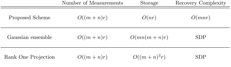
TABLE 1 : Comparison Between Three Sensing Schemes . . . 48
LIST OF ILLUSTRATIONS
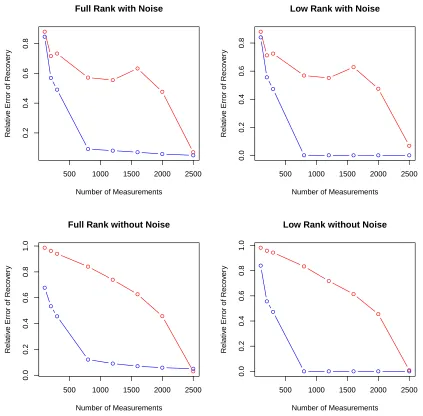
FIGURE 1 : Comparison Between Proposed Scheme and Gaussian Ensemble . 53
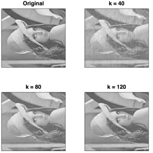
FIGURE 2 : Recovery of Lena with Different Sampling Parameters . . . 55
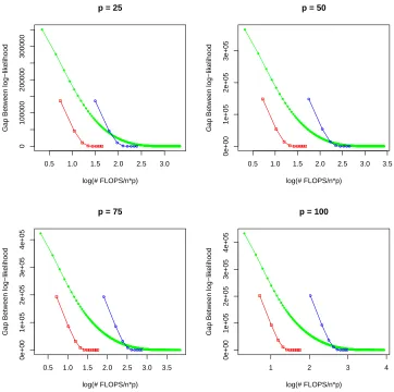
FIGURE 3 : Results for Simulation Studies . . . 75
CHAPTER 1 : Introduction
In the first part of this dissertation we study two problems in sequential decision making,
where the decision maker faces uncertain outcomes and has to make decisions throughout
a discrete time horizon. We are most interested in the asymptotic performance of certain
strategies carried out by the decision maker.
In Chapter 2, we consider the sequential monotone subsequence selection problem, where the
decision maker faces the valuesπ[1],π[2], ... from a random permutationπ: [1 :n]→[1 :n]
one by one and, when shown the value π[i] at timei, must decide (once and for all) either
to accept or reject π[i] as element of the selected increasing subsequence. One can easily
relate this to a similar problem, where we consider sequential selection from a sequence ofn
independently uniformly distributed random variablesX1,X2, ...,Xn instead of a random
permutation. It was established by Samuels and Steele (1981) that
s(n)∼sˆ(n)∼√2n (1.1)
where s(n) and ˆs(n) denote the expected value of optimal selection from a random
per-mutation andnindependent and identically distributed samples respectively. Nevertheless,
there is a flurry of literature on characterizing ˆs(n) while few have focused on analyzing
s(n). To the best of our knowledge, there is no finer analysis of s(n) than (1.1). Given the
similarities that lie between these two problems, one might hope there is a definite
relation-ship betweens(n) and ˆs(n), but this is far from intuitive. Our contributions are two-fold: in
the first place we proved thats(n)≥sˆ(n), which implies that the decision maker is better
off in the permutation problem; secondly, we managed to quantify the extent to which it is
better. Specifically, s(n) is larger by at least (1/6) logn+O(1).
When the decision maker adopts the greedy strategy, the selected values correspond to
distributed samples is well studied by R´enyi (1962). In Chapter 3 we generalize classical
records to relative records and consider the multiplicative relaxations and constrictions of
the number of records, which have not been studied previously and lead to novel phenomena.
First, the number of relative records is no longer independent of the distribution function.
Moreover, the asymptotic behaviour is unlike the behavior that one finds for the classical
record process. In the relaxed case, we find a central limit theorem (CLT) with a different
normalization than Renyi’s classical CLT, and in the constricted case we find convergence
in distribution to an unbounded random variable.
The big data era has posed tremendous challenge to traditional non-scalable and
compu-tationally inefficient algorithms. Random projection and randomized subsampling are two
powerful tools that have found their applications in a variety of problems. Based on these
two ideas, in the second part of this dissertation we put forward two randomized algorithms
addressing the low rank matrix recovery problem and large-scale estimation of generalized
linear model respectively.
Exploration of low-rank structure is of great significance and interest in a wide range of
ap-plications. In Chapter 4, we propose a randomized two-step sensing scheme for the low-rank
matrix recovery problem, which requires far less storage space and has much lower
com-putational complexity compared with other state-of-art methods based on nuclear norm
minimization. Besides exact recovery in the ideal low-rank and noiseless case, the proposed
procedure is applicable to cases where the underlying matrix has full rank with decaying
singular values and where the measurements suffer from noise. Expectation and
concen-tration error bounds for both the spectral norm and the Frobenious norm are established.
Finally, numerical experiments are given to support the theory.
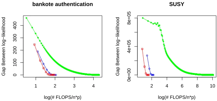
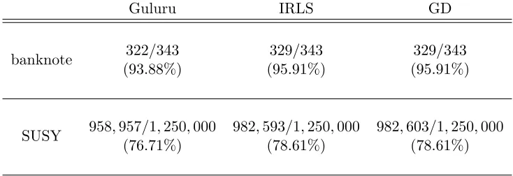
In Chapter 5, we propose a fast iterative reweighted least squares algorithm,Guluru, based
on subsampled randomized Hadamard transform, to solve a wide class of generalized
lin-ear models under the large n, large p and n p setting, where, as usual, n denotes the
algorithm reduces the computational complexity fromO(np2) toO(np). We provide
theo-retical guarantees that the log-likelihood achieved by Guluru upon convergence is at most
O(p2/nr2) away from the maximum log-likelihood, where r is the subsampling ratio. We
also prove that the final estimator of Guluru is only O(p/nr) away from the maximum
likelihood estimator. Extensive empirical studies demonstrate the competitive performance
CHAPTER 2 : Sequential Selection of a Monotone Subsequence
From a Random Permutation
2.1. Sequential Subsequence Problems
In the classical monotone subsequence problem, one chooses a random permutation π: [1 :
n]→[1 :n], and one considers the length of its longest increasing subsequence,
Ln= max{k:π[i1]< π[i2]<· · ·< π[ik] where 1≤i1< i2· · ·< ik≤n}.
On the other hand, in thesequential monotone subsequence problem one views the values
π[1], π[2], ... as though they were presented over time to a decision maker who, when
shown the value π[i] at timei, must decide (once and for all) either to accept or rejectπ[i]
as element of the selected increasing subsequence.
The decision to accept or reject π[i] at time i is based on just the knowledge of the time
horizonnand the observed valuesπ[1], π[2], . . . , π[i]. Thus, in slightly more formal language,
the sequential selection problems amounts to the consideration of random variables of the
form
Lτn= max{k:π[τ1]< π[τ2]<· · ·< π[τk] where 1≤τ1< τ2· · ·< τk≤n}, (2.1)
where the indicesτi,i= 1,2, . . . are stopping times with respect to the increasing sequence
of σ-fields Fk = σ{π[1], π[2], . . . , π[k]}, 1 ≤ k ≤ n. We call a sequence of such stopping
times afeasible selection strategy, and, if we use τ as a shorthand for such a strategy, then
the quantity of central interest here can be written as
s(n) = sup τ E
where one takes the supremum over all feasible selection strategies.
It was conjectured in Baer and Brock (1968) that
s(n)∼√2n asn→ ∞, (2.3)
and a proof of this relation was first given in Samuels and Steele (1981). A much simpler
proof of (2.3) was later given by Gnedin (2000) who made use of a recursion that had been
used for numerical computations by Baer and Brock (1968). The main purpose of this note
is to show how by a more sustained investigation of that recursion one can obtain a two
term expansion.
Theorem 1 (Sequential Selection from a Random Permutation). Forn→ ∞ one has the
asymptotic relation
s(n) =√2n+1
6logn+O(1). (2.4)
Given what is known for some closely related problems, the explicit second order term
(logn)/6 gives us an unanticipated bonus. For comparison, suppose we consider sequential
selection from a sequence of n independently uniformly distributed random variables X1,
X2, ...,Xn. In this problem a feasible selection strategyτ is again expressed by an increasing
sequence of stopping timesτj,j = 1,2, . . ., but now the stopping times are adapted to the
increasing σ-fields Fbj =σ{X1, X2, . . . , Xj}. The analog of (2.1) is then
b
Lτn = max{k:Xτ1 < Xτ2 <· · ·< Xτk where 1≤τ1 < τ2· · ·< τk≤n}, (2.5)
and the analog of (2.2) is given by
b
s(n) = sup τ E
Bruss and Robertson (1991) found that for bs(n) one has a uniform upper bound
b
s(n)≤√2n for all n≥1, (2.6)
so, by comparison with (2.4), we see there is a sense in which sequential selection of a
monotone subsequence from a permutation iseasier than sequential selection from an
inde-pendent sequence. In part, this is intuitive; each successive observation from a permutation
gives useful information about the subsequent values that can be observed. By (2.4) one
quantifies how much this information helps, and, so far, we have only an analytical
under-standing of the source of (1/6) logn. A genuinely probabilistic understanding of this term
remains elusive.
Since (2.6) holds for all nand since (2.4) is only asymptotic, it also seems natural to ask if
there is a relation betweensb(n) and s(n) that is valid for all n. There is such a relation if
one gives up the logarithmic gap.
Theorem 2 (Selection for Random Permutations vs Random Sequences). One has for all
n= 1,2, . . . that
b
s(n)≤s(n).
Here we should also note that much more is known aboutbs(n) than just (2.6); in particular,
there are several further connections between s(n) andbs(n). These are taken up in a later
section, but first it will be useful to give the proofs of Theorems 1 and 2.
The larger context for the problems studied here is the theory of Markov decision processes
(or MDPs) which is closely tied to the theory of optimal stopping and the theory of on-line
algorithms (cf. Puterman (1994), Shiryaev (2008), and Flat and Woeginger (1998)). The
traditional heart of the theory of MDPs is the optimality equation (or Bellman equation)
which presents itself here as the identity (2.7). One of our main motivations has been the
expectation that (2.7) gives one an appropriate path for examining how one can extract
oc-cur in the theory of MDPs. In this respect, it seems hopeful that tools that parallel the
comparison principles of Section 2.3 and the approximate solutions of Section 2.4 may be
broadly applicable, although the details will necessarily vary from problem to problem.
The proof of Theorem 1 takes most of our effort, and it is given over the next few
sec-tions. Section 2.2 develops the basic recurrence relations, and Section 2.3 develops stability
relations for these recursions. In Section 2.4 we then do the calculations that support a
candidate for the asymptotic approximation ofs(n), and we complete the proof of Theorem
1. Our arguments conclude in Section 2.5 with the brief — and almost computation free —
proof of Theorem 2. Finally, in Section 2.6 we discuss further relations betweens(n),bs(n),
and some other closely related quantities that motivate consideration of two open problems.
2.2. Recurrence Relations
One can get a recurrence relation for s(n) by first step analysis. Specifically, we take a
random permutationπ: [1 :n+ 1]→[1 :n+ 1], and we consider its initial valueπ[1] =k. If
we rejectπ[1] as an element of our subsequence, we are faced with the problem of sequential
selection from the reduced random permutationπ0 on ann-element set. Alternatively, if we
choose π[1] = k as an element of our subsequence, we are then faced with the problem of
sequential selection for a reduced random permutationπ00 of the set{k+ 1, k+ 2, . . . , n+ 1}
that hasn+ 1−kelements. By taking the better of these two possibilities, we get from the
uniform distribution ofπ[1] that
s(n+ 1) = 1
n+ 1
n+1
X
k=1
max{s(n),1 +s(n+ 1−k)}. (2.7)
From the definition (2.2) of s(n) one has s(1) = 1, so subsequent values can then be
computed by (2.7). For illustration and for later discussion, we note that one has the
n 1 2 3 4 5 6 7 8 9 10
s(n) 1 1.5 2 2.375 2.725 3.046 3.333 3.601 3.857 4.098
√
2n 1.414 2 2.449 2.828 3.162 3.464 3.742 4 4.243 4.472.
Here we observe that for the 10 values in the table one has s(n) ≤√2n, and, in fact, this
relation persists for all 1≤n≤174. Nevertheless, forn= 175 one has√2n < s(n), just as
(2.4) requires for all sufficiently large values of n.
We also know from (2.2) that the mapn7→s(n) is strictly monotone increasing, and, as a
consequence, the recursion (2.7) can be written a bit more simply as
s(n+ 1) = 1
n+ 11max≤k≤n
(
(n−k+ 1)s(n) +
n
X
i=n−k+1
{s(i) + 1}
)
(2.8)
= 1
n+ 11max≤k≤n
(
(n−k+ 1)s(n) +k+
n
X
i=n−k+1 s(i)
)
.
In essence, this recursion goes back to Baer and Brock (1968, p. 408), and it is the basis of
most of our analysis.
2.3. Comparison Principles
Given a mapg:N→Rand 1≤k≤n, it will be convenient to set
H(n, k, g) =k+ (n−k+ 1)g(n) +
n
X
i=n−k+1
g(i), (2.9)
so the optimality recursion (2.8) can be written more succinctly as
s(n+ 1) = 1
n+ 11max≤k≤nH(n, k, s). (2.10)
The next two lemmas make rigorous the idea that if gis almost a solution of (2.10) for all
Lemma 2.1 (Upper Comparison). If δ :N→R+,1≤g(1) +δ(1), and
1
n+ 11max≤k≤nH(n, k, g)≤g(n+ 1) +δ(n+ 1) for alln≥1, (2.11)
then one has
s(n)≤g(n) +
n
X
i=1
δ(i) for all n≥1. (2.12)
Proof. We set ∆(i) =δ(1) +δ(2) +· · ·+δ(i), and we argue by induction. Specifically, using
(2.12) for 1≤i≤nwe have
H(n, k, s) =k+ (n−k+ 1)s(n) +
n
X
i=n−k+1 s(i)
≤k+ (n−k+ 1)(g(n) + ∆(n)) +
n
X
i=n−k+1
{g(i) + ∆(i)}
so by monotonicity of ∆(·) we have
1
n+ 1H(n, k, s)≤ 1
n+ 1H(n, k, g) + ∆(n).
Now, when we take the maximum over k ∈ [1 : n], the recursion (2.8) and the induction
condition (2.11), give us
s(n+ 1)≤ 1
n+ 11max≤k≤nH(n, k, g) + ∆(n)
≤g(n+ 1) +δ(n+ 1) + ∆(n) =g(n+ 1) + ∆(n+ 1),
so induction establishes (2.12) for alln≥1.
Naturally, there is a lower bound comparison principle that parallels Lemma 2.1. The
statement has several moving parts, so we frame it as a separate lemma even though its
Lemma 2.2 (Lower Comparison). If δ:N→R+, g(1)−δ(1)≤1, and
g(n+ 1)−δ(n+ 1)≤ 1
n+ 11max≤k≤nH(n, k, g) for alln≥0,
then one has
g(n)−
n
X
i=1
δ(i)≤s(n) for all n≥1.
2.4. An Approximation Solution
We now argue that the function f :N→R defined by
f(n) =√2n+1
6logn, (2.13)
gives one an approximate solution of the recurrence equation (2.8) forn7→s(n).
Proposition 2.3. There is a constant 0< B <∞ such that for all n≥1, one has
−Bn−3/2 ≤ 1
n+ 1
max
1≤k≤nH(n, k, f)
−f(n+ 1)≤Bn−3/2. (2.14)
First Step: Localization of the Maximum
To deal with the maximum in (2.14), we first estimate
k∗(n) = locmaxk H(n, k, f).
From the definition (2.9) of H(n, k, f) we find
H(n, k+ 1, f)−H(n, k, f) = 1−f(n) +f(n−k),
of k; accordingly, we also have the representation
k∗(n) = 1 + max{k: 0≤1−f(n) +f(n−k)}. (2.15)
Now, for each n= 1,2, . . . we then consider the functionDn: [0, n]→R defined by setting
Dn(x) = 1−f(n) +f(n−x) = 1− {
√
2n−p2(n−x)} −1
6{logn−log(n−x)}.
This function is strictly decreasing withDn(0) = 1 and Dn(n) =−∞, so there is a unique
solution of the equation Dn(x) = 0. For x∈[0, n) we also have the easy bound
Dn(x) = 1−
1 2
Z 2n
2(n−x) 1 √
udu−
1
6log(n/(n−x))≤1−
x √
2n.
This gives usDn(
√
2n)≤0, so by monotonicity we have xn≤
√ 2n.
To refine this bound to an asymptotic estimate, we start with he equationDn(xn) = 0 and
we apply Taylor expansions to get
1 =√2nn1−(1−xn/n)1/2
o
−1
6log(1−xn/n)
=√2nnxn
2n+O(x 2
n/n2)
o
+O(xn/n).
By simplification, we then get
√
2n=xn+O(x2n/n) +O(xn/n1/2) =xn+O(1), (2.16)
where in the last step we used our first boundxn≤
√ 2n.
Finally, by (2.16) and the characterization (2.15), we immediately find the estimate that
Lemma 2.4. There is a constant A >0 such that for all n≥1, we have
√
2n−A≤k∗(n)≤√2n+A. (2.17)
Remark 2.5. The relations (2.16) and (2.17) can be sharpened. Specifically, if we use a
two-term Taylor series with integral remainders, then one can show√2n−2≤xn. Since we
already know thatxn≤
√
2n, we then see from the characterization (2.15) and integrality of
k∗(n) that we can takeA= 2 in Lemma 2.4. This refinement does not lead to a meaningful
improvement in Theorem 1, so we omit the details of the expansions with remainders.
Completion of Proof of Proposition 2.3
To prove Proposition 2.3, we first note that the definition (2.9) of H(n, k, f) one has for all
1≤k≤nthat
1
n+ 1H(n, k, f) =f(n) + 1
n+ 1 (
k−
k−1
X
i=1
(f(n)−f(n−i)) )
(2.18)
The task is to estimate the right-hand side of (2.18) whenk=k∗(n) and k∗(n) is given by
(2.15).
For the moment, we assume that one has k ≤D√n where D > 0 is constant. With this
assumption, we find that after making Taylor expansions we get from explicit summations
that
k−1
X
i=1
(f(n)−f(n−i)) =
k−1
X
i=1
√
2n−p2(n−i)+
k−1
X
i=1
logn
6 −
log(n−i) 6
=
k−1
X
i=1
i √
2n+ i2
4n√2n+O
i3 n5/2
+
k−1
X
i=1
i
6n+O
i2 n2
= (k−1)k 2√2n +
(k−1)k(2k−1) 24n√2n +
(k−1)k
12n +O(n
−1/2), (2.19)
We now define r(n) by the relation k∗(n) = √2n+r(n), and we note by (2.17) that
|r(n)| ≤A. Direct algebraic expansions then give us the elementary estimates
(k∗(n)−1)k∗(n)
12n =
1
6 +O(n −1/2)
and
(k∗(n)−1)k∗(n)(2k∗(n)−1)
24n√2n =
1
6+O(n −1/2),
where in each case the implied constant depends only onA.
Estimation of the first summand of (2.19) is slightly more delicate than this since we need
to account for the dependence of this term on r(n); specifically we have
(k∗(n)−1)k∗(n)
2√2n =
√
2n+r(n)−1 √
2n+r(n)
2√2n
=pn/2 +r(n)−1
2 +O(n −1/2).
Now, for a pleasing surprise, we note from the last estimate and from the definition ofk∗(n)
and r(n) that we have cancelation of r(n) when we then compute the critical sum; thus,
one has simply
k∗(n)−
k∗(n)−1
X
i=1
(f(n)−f(n−i)) =pn/2 +1
6+O(n
−1/2). (2.20)
Finally, from the formula (2.13) forf(·), we have the Taylor expansion
f(n+ 1)−f(n) = √1 2n+
1
6n +O(n
−3/2), (2.21)
us the estimate
1
n+ 1
max
1≤k≤nH(n, k, f)
−f(n+ 1)
= 1
n+ 1
p
n/2 +1
6 +O(n −1/2)
+f(n)−f(n+ 1) =O(n−3/2).
Here the implied constant is absolute, and the proof of Proposition 2.3 is complete.
Completion of Proof of Theorem 1
Lemmas 2.1 and 2.2 combine with Proposition 2.3 to tell us that by summing the sequence
n−3/2,n= 1,2, . . . and by writingζ(z) = 1 + 2−z+ 3−z+· · · one has
|s(n)−f(n)| ≤ζ(3/2)B ≤(2.62)B for alln≥1.
This is slightly more than one needs to complete the proof of Theorem 1.
2.5. Proof of Theorem 2
The sequential monotone selection problem is a finite horizon Markov decision problem with
bounded rewards and finite action space, and for such problems it is known one cannot
improve upon an optimal deterministic strategy by the use of strategies that incorporate
randomization, Bertsekas and Shreve (1978, Corollary 8.5.1)cf.. The proof of Theorem 2
exploits this observation by constructing a randomized algorithm for the sequential selection
of a monotone subsequence from a random permutation.
We first recall that ifei,i= 1,2, . . . , n+1 are independent exponentially distributed random
variables with mean 1 and if one sets
Yi=
e1+e2+· · ·+ei
e1+e2+· · ·+en+1
,
(X(1), X(2), . . . , X(n)) of an i.i.d. sample of size n from the uniform distribution (see e.g.
Feller (1971), p. 77). Next we let A denote an optimal algorithm for sequential selection
of an increasing subsequence from an independent sampleX1, X2, . . . , Xnfrom the uniform
distribution, and we let τ(A) denote the associated sequence of stopping times. If Lb τ(A)
n
denotes the length of the subsequence that is chosen from from X1, X2, . . . , Xn when one
follows the strategy τ(A) determined by A, then by optimality of A for selection from
X1, X2, . . . , Xnwe have
b
s(n) = sup τ E
[Lbτn] =E[Lbτn(A)].
We use the algorithmAto construct a new randomized algorithmA0 for sequential selection
of an increasing sequence from a random permutation π : [n] 7→ [n]. First, the decision
maker generates independent exponential random variablesei,i= 1,2, . . . , n+ 1 as above.
This is done off-line, and this step can be viewed as an internal randomization.
Now, for i= 1,2, . . . , n, when we are presented with π[i] at timei, we computeXi =Yπ[i].
Finally, if at timeithe valueXi would be accepted by the algorithmA, then the algorithm
A0 accepts π[i]. Otherwise the newly observed value π[i] is rejected. By our construction
we have
E[Lτ(A
0)
n ] =E[Lbτn(A)] = b
s(n). (2.22)
Moreover, A0 is a randomized algorithm for construction an increasing subsequence of a
random permutation π. By definition, s(n) is the expected length of a monotone
subse-quence selected from a random permutation by an optimal deterministic algorithm, and by
our earlier observation, the randomized algorithm A0 cannot do better. Thus, from (2.22)
2.6. Further Developments and Considerations
The uniform upper bound (2.6) was obtained by Bruss and Robertson (1991) as a
conse-quence of a bound on the expected value of the random variable
N(s) = max
|A|:X
i∈A
Xi ≤s
where the observations{Xi :i∈[1 :n]} have a common continuous distribution with
sup-port in [0,∞). This bound was extended in Steele (2016) to accommodate non-identically
distributed random variables, and, as a consequence, one finds some new bounds for the
sequential knapsack problems.
On the other hand, this extension does not help one to refine or generalize (2.6), since, as
Coffman et al. (1987) first observed, the sequential knapsack problem and the sequential
increasing subsequence problem are equivalent only when the observations are uniformly
and identically distributed. Certainly, one may consider the possibility of analogs of (2.6)
for non-identically distributed random variables, but, as even deterministic examples show,
the formulation of such analogs is problematical.
Here we should also note that Gnedin (1999) gave a much different proof of (2.6), and,
moreover, he generalized the bound in a way that accommodates random samples with
random sizes. More recently, Arlotto et al. (2015a) obtained yet another proof (2.6) as
a corollary to bounds on the quickest selection problem, which is an informal dual to the
traditional selection problem.
Since the bound (2.6) is now well understood from several points of view, it is reasonable
to ask about the possibility of some corresponding uniform bound ons(n). The numerical
values that we noted after the recursion (2.6) and the relation
s(n) = √
2n+ 1
from Theorem 1 both tell us that one cannot expect a uniform bound for s(n) that is as
simple as that for bs(n) given by (2.6). Nevertheless, numerical evidence suggests that the
O(1) term in (2.23) is always negative. The tools used here cannot confirm this conjecture,
but the multiple perspectives available for (2.6) give one hope.
A closely related issue arises forbs(n) when one considers lower bounds. Here the first steps
were taken by Bruss and Delbaen (2001) who considered i.i.d. samples of sizeNν whereNν
is an independent random variable with the Poisson distribution with mean ν. If now we
write bs(ν) for the expected value of the length of the subsequence selected by an optimal
algorithm in the Bruss-Delbaen framework, then they proved that there is a constantc >0
such that
√
2ν−clogν≤bs(ν);
moreover, Bruss and Delbaen (2004) subsequently proved that for the optimal feasible
strategyτ∗ = (τ1, τ2, . . .) the random variable
b
Lτ∗
Nν = max{k:Xτ1 < Xτ2 <· · ·< Xτk where 1≤τ1< τ2· · ·< τk≤Nν},
also satisfies a central limit theorem. Arlotto et al. (2015b) considered the de-Poissonization
of these results, and it was found that one has the corresponding CLT for Lbτn∗ where the
sample size nis deterministic. In particular, one has the bounds
√
2n−clogn≤sb(n)≤√2n.
Now, by analogy with (2.23), one strongly expects that there is a constant c >0 such that
b
s(n) = √
2n−clogn+O(1). (2.24)
Still, a proof this conjecture is reasonably remote, since, for the moment, there is not even
For a second point of comparison, one can recall thenon-sequential selection problem where
one studies
`(n) =E[max{k:Xi1 < Xi2 < . . . < Xik, 1≤i1< i2 <· · ·< ik≤n}].
Through a long sequence of investigations culminating with Baik et al. (1999), it is now
known that one has
`(n) = 2√n−αn1/6+o(n1/6), (2.25)
where the constant α = 1.77108... is determined numerically in terms of solutions of a
Painlev´e equation of type II. Romik (2014) gives an elegant account of the extensive
tech-nology behind (2.25), and there are interesting analogies between`(n) ands(n).
Neverthe-less, a proof of the conjecture (2.24) seems much more likely to come from direct methods
like those used here to prove (2.23).
Finally, one should note that the asymptotic formulas forn7→`(n),n7→s(n), andn7→bs(n)
all suggest that these maps are concave, but so far only n7→ bs(n) has been proved to be
CHAPTER 3 : Relative Records: Relaxed or Constrained
3.1. Relaxed or Constrained Sequential Selection Processes
LetXi,i= 1,2, . . .be a sequence of independent random variables with a common
continu-ous distributionF with support in [0,∞), and let ρdenote a non-negative constant. Next,
we set τ1= 1, and we define a sequence of stopping times by taking
τk= min{j:Xj ≥ρXτk−1} fork >1. (3.1)
The random variables of main interest here are then given by
Rn(ρ) = max{k:τk≤n}. (3.2)
Whenρ= 1 the timesτk,k= 1,2, . . .are precisely the times at which new record values are
observed, and Rn(1) is the total number of records that are observed in the time interval
[1 :n] ={1,2, . . . , n}.
The random variableRn(1) has been well understood for a long time. In particular, R´enyi
(1962) found among other things that E[Rn(1)] ∼logn and Var[Rn(1)]∼logn; moreover,
he found that one has
Rn(1)√ −logn
logn ⇒N(0,1), (3.3)
where, as usual, the symbol⇒ denotes convergence in distribution andN(0,1) denotes the
standard Gaussian distribution.
The cases ρ ∈ (0,1) and ρ ∈ (1,∞) have not been considered previously, and they lead
to some novel phenomena. First, the distribution of Rn(ρ) is no longer independent of F.
Moreover, one finds that the asymptotic behavior is unlike the behavior that one finds for
The most interesting case is when ρ ∈ (0,1) where, in comparison to the classical record
process, one hasrelaxed the condition that is imposed on the condition for sequential
selec-tions. In this case one again has a central limit theorem, but it differs substantially from
Renyi’s. In particular, forρ∈(0,1) the mean and variance grow linearly and the summands
are not independent.
For the sake of brevity, we say a distribution function is in theselection class SL if there is
an L ∈ (0,∞) such that F(0) = 0, F(L) = 1, and F is continuous and strictly monotone
on (0, L). For example, the uniform distribution on [0,1] is in S1, and for any L > 0 the
truncated exponential distributionF(x) = (1−e−x)/(1−e−L) is inSL. For these examples,
one has a density, but, in general, a distribution inSL need not have a density.
Theorem 3(Mean, Variance, and CLT when 0< ρ <1). IfXi,i= 1,2, . . .are independent
and if F ∈ SL, then there are constants µρ(F)>0 and σρ(F)>0 such that
E[Rn(ρ)]∼nµρ(F) and Var[Rn(ρ)]∼nσρ2(F), (3.4)
and one has a central limit theorem
Rn(ρ)−nµρ(F)
σρ(F)
√
n ⇒N(0,1). (3.5)
After we develop some useful connections with the theory of Markov chains in Sections 3.2
and 3.3, the proof of Theorem 3 is given in Section 3.4. The main issues are the proofs of the
relations (3.4) and the proof of σ2
ρ(F) >0. Once these facts are in hand, the convergence
(3.5) then follows from general theory; for example, one can obtain (3.5) directly from
Arlotto and Steele (2016) Theorem 1, Corollary 2. Alternatively, with a page or two of
extra work, one can obtain (3.5) by first generalizing other known central limit theorems
for additive functionals of Markov processes. In either case, the proof that σρ2(F)>0 is a
make-or-break step.
intractable. Nevertheless, in the case of most interest when F is the uniform distribution
U on [0,1], there is at least an explicit series formula for the mean.
Theorem 4 (Moments for Uniform Distribution). If ρ∈(0,1)and if the random variables
Xi, i= 1,2, . . . have the uniform distribution U on[0,1], then we have
µρ(U) = 1−
ρ
2−
ρ
3
ρ−ρ 2
2
−ρ
4
ρ−ρ 2
2 ρ−
ρ3
3
−ρ
5
ρ−ρ 2
2 ρ−
ρ3
3 ρ−
ρ4
4
· · ·
(3.6)
The proof of Theorem 4 is then given in Section 3.5 where we also develop an equation
of the pantograph type for the stationary distribution of the driving Markov chain. We
do not solve this equation, but we use it to derive the Mellin transform for the stationary
distribution. This we use in turn to get the required explicit formula (3.6) forµρ(U).
While there is little hope of finding a correspondingly explicit representation forσ2
ρ(F) even
for F =U, we do find in Section 3.4 that there is a useful series representation (3.26) for
σρ2(F).
When ρ > 1, one no longer has a central limit theorem. Instead one has almost sure
convergence to an unbounded random variable with a well-behaved moment generating
function.
Theorem 5 (Distributional Limit when ρ > 1). If F ∈ SL and if F(x) = O(x) in the
neighbourhood of0, then for eachρ >1 there exists an unbounded random variableNρwith
moment generating function
E[exp(sNρ)]<∞ for |s|<logρ, (3.7)
such that with probability one Rn(ρ)%Nρ as n→ ∞.
The case ρ > 1 of the sequential selection process can be viewed as a “degenerate case”
where one no longer has a central limit theory. This is less interesting than the cases ρ= 1
we give a brief — but complete — analysis of this case in Section 3.7.
Section 3.8 then gives refinements of several kinds of Renyi’s classic formula for the expected
number of records. For example, consider the numberRxn(1) of records that are larger than
x. When F is the uniform distribution on [0,1], we find
E[Rxn(1)] =Hn− n
X
k=1 xk
k . (3.8)
This formula recaptures Renyi’s classic harmonic sum when we setx= 0, yet its proof shares
nothing in common with classic argument of R´enyi (1962). Moreover, the methods that lead
one to (3.8) yield further generalizations for the quantities E[Rxn(ρ)] and limn{E[Rxn(ρ)]−
E[Ryn(ρ)]} that are defined more fully in Section 3.8.
In Section 3.9 we make more explicit the senses in which the values chosen by the selection
process (3.1) can be viewed as relaxed or constrained records. We also show how in the
relaxed caseρ∈(0,1), the selected values can differ greatly from any notion of approximate
record, even though our selection process and various approximate record processes may
both contain the record process as limiting cases.
3.2. Representation as a Markov Additive Functional
For k = 1,2, . . . we take Yk to be the last value that has been accepted by the selection
process during the time interval [1 :k]; that is, we set
Yk=Xτj where j= max{m:τm ≤k}.
The valuesYk,k= 1,2, . . .determine a Markov chain where if one is in statexthen one stays
in statex with probabilityF(ρx) and with probability 1−F(ρx) one moves to a point yin
the set [ρx,1]\ {x}that is chosen according to the probability measuredF(y)/(1−F(ρx)).
kernel
Kρ,F(x, A) =F(ρx)1(x∈A) +
Z L
ρx
1(y∈A)dF(y). (3.9)
Now, in terms of the Markov chain{Yk: 0 = 1,2, . . .} we have the representation
Rn(ρ) = n
X
k=1
1[Yk6=Yk−1], (3.10)
since we accept a new value precisely at the times when the state of the chain{Yn}changes.
Most of Theorem 3 follows from this representation after we establish a few analytic
prop-erties of the Markov chain{Yn}.
Remark 3.1. Here one should note that by definitionRn(ρ) is a function of the independent
random variables {X1, X2, . . . Xn}, and we simply write E[Rn(ρ)] and Var[Rn(ρ)] when
Rn(ρ) is viewed in this way. On the other hand, by the representation (3.10), we can also
view Rn(ρ) as a function of {Y1, Y2, . . . , Yn} and the distribution of this sequence depends
on the initial distribution of the Markov chain. When we take the second point of view it is
natural (and necessary) to writeEµ[Rn(ρ)] and Varµ[Rn(ρ)] wheneverY0has the distribution
µ. By construction, we always have Var[Rn(ρ)] = Var0[Rn(ρ)] andE[Rn(ρ)] =E0[Rn(ρ)].
3.3. The Dobrushin Coefficient and Its Consequences
There are several ways one can investigate the Markov chain defined by (3.9), but here it
is especially efficient to first estimate the Dobrushin coefficient.
Definition 3.2 (Dobrushin Coefficient). If K is a Markov transition function on a Borel
state spaceX and ifB(X) denotes the collection of Borel subsets ofX, then the Dobrushin
coefficient δ(K) of the kernel K is defined by
δ(K) = sup
x1,x2∈X, A∈B(X)
|K(x1, A)−K(x2, A)|.
kernel given by (3.9), then one has
δ(Kρ,F)≤F(ρL)<1. (3.11)
Proof. If we assumex1< x2, then for any Borel setA⊂[0, L] we have from (3.9) that
∆def= Kρ,F(x1, A)−Kρ,F(x2, A)
=F(ρx1)1(x1 ∈A) +
Z 1
ρx1
1(y∈A)dF(y)−F(ρx2)1(x2 ∈A)−
Z 1
ρx2
1(y∈A)dF(y)
=F(ρx1)1(x1 ∈A)−F(ρx2)1(x2 ∈A) +
Z ρx2
ρx1
1(y∈A)dF(y).
After majorizing the positive terms, we see from monotonicity ofF that
∆≤F(ρx1) +{F(ρx2)−F(ρx1)}=F(ρx2)≤F(ρL).
On the other hand, if we keep just the one negative terms, then we have
∆≥ −F(ρx2)≥ −F(ρL),
and these two bounds on ∆ complete the proof of (3.11).
Nagaev (2015) proved that for any Markov chain with kernelK and Dobrushin coefficient
δ(K) < 1, there is a probability measure ν on the state space X that is stationary under
K, and, most notably, if K(n) denotes the n step transition kernel, then one has the total
variation bound
|K(n)(x, A)−ν(A)| ≤2[δ(K)]n for all x∈ X and A∈ B(X). (3.12)
Now, we let {Zn : n = 0,1,2, . . .} be the Markov chain associated with the kernel K,
Z0 = x ∈ X or Z0 ∼ ν. By the total variation bound (3.12) and approximation by step
functions, one can then check that for any bounded measurable g:D=X4 →
R, one has
for any fixed 0≤i≤j≤k and n→ ∞ that
Ex[g(Zn, Zn+i, Zn+j, Zn+k)]−Eν[g(Z0, Zi, Zj, Zk)] =O(||g||∞[δ(K)]n), (3.13)
where here we set||g||∞= supv∈D|g(v)|.
The implied constant in (3.13) is absolute; in fact, it can be taken to be 4. Naturally, we
also have analogous relations for functions of fewer than four variables or more than four
variables. Here we only need (3.13) and its analog for functions of two variables.
3.4. Whenρ <1: Proof of Theorem 3
We now restrict attention to the Markov chain with transition kernel Kρ,F(·,·) given by
(3.9). By the bound (3.11) we have δ ≡δ(Kρ,F)<1, so the stationary distribution exists.
We consider two initial distributions: in the first case we take Y0 ≡0; and in the second
case we assume that Y0 has the stationary distribution ν. By the two variable analog of
(3.13) forg(Yn, Yn+1) =1(Yn6=Yn+1) we have
E0[1(Yk−16=Yk)] =Eν[1(Y0 6=Y1)] +O(δk). (3.14)
From (3.14) and the representation (3.10), we see by geometric summation that
E0[Rn(ρ)] = n
X
k=1
E01([Yk−1 6=Yk)] =nEν[1(Y06=Y1)] +O(1) (3.15)
=n
Z
X Z
X
1[s6=t]Kρ,F(s, dt)dν(s) +O(1),
where the double integral is justEν[1(Y0 6=Y1)] written in longhand. This gives us the first
us that in (3.4) we have
µρ(F) =
Z
X Z
X
1[s6=t]Kρ,F(s, dt)dν(s). (3.16)
To find the asymptotic variance ofRn(ρ), we introduce two sequences of random variables:
Uk=1[Yk−16=Yk]−E0(1[Yk−16=Yk]) andVk =1[Yk−16=Yk]−Eν(1[Yk−1 6=Yk]).
Both Uk and Vk are functions of the Markov process {Yk :k = 0,1, . . .}, so in particular,
both{Un}and{Vn}depend on the initial valueY0. For clarity one should note thatUkhas
mean zero when Y0 ≡0 and Vk has mean zero when Y0 follows the stationary distribution
ν.
The random variablesUk and Vk differ by a constant that depends onk, and by (3.14) the
constant is not larger thanO(δk). Thus, by the representation (3.10), we have
Var[Rn(ρ)] = Var0[Rn(ρ)] =E0
n
X
k=1 Uk
2
=E0
n
X
k=1 Vk
2
+O(1). (3.17)
Now, when we expand the second sum in (3.17) and write
E0
n
X
k=1 Vk
2
=
n
X
k=1
E0[Vk2] + 2 n−1
X
i=1
n−i
X
j=1
E0[ViVi+j]def= An+Bn. (3.18)
To estimate the first sum An of (3.18), we apply (3.13) just as we did in the derivation of
(3.14), and this time we find
Summation then gives us
An=nEν[V12] +O(1). (3.19)
To deal with the double sum Bn, we first need a lemma to help us estimate the summands
of Bn.
Lemma 3.4. For any initial distribution µ one has
Eµ[ViVi+j] =O(δj) for alli, j≥0. (3.20)
Proof. To exploit the Markov property for the chain {Yn:n= 0,1, . . .}, we first condition
on Yi−1 and Yi and note that
Eµ[ViVi+j] =Eµ[ViEµ[Vi+j|Yi−1, Yi]] =Eµ[ViEµ[Vi+j|Yi]] =Eµ[ViEYi[Vj]]. (3.21)
If we use (3.13) as before, then we see that for all x∈ X we have
Ex[Vn] =Eν[Vn] +O(δn),
and the implied constant does not depend on x. When we insert this in (3.21) and recall
that the definition ofVngives us Eν[Vn] = 0, the proof of the lemma is complete.
Lemma 3.4 helps us deal with cross terms with large j, but we also need a relation that
deals with arbitrary j. Here, we again use (3.13) to get for allj≥0 that
E0[ViVi+j] =Eν[ViVi+j] +O(δi) =Eν[V1V1+j] +O(δi). (3.22)
and then apply (3.22) to the rest to obtain
Bn= 2 n−1
X
j=1
j
X
i=1
O(δj) + 2
b(n−1)/2c X
j=1
n−1
X
i=j+1
Eν[V1V1+j] +O(δi)
. (3.23)
We have the sums
n−1
X
j=1
j
X
i=1
O(δj) =
n−1
X
j=1
O(jδj) =O(1),
b(n−1)/2c X
j=1
n−1
X
i=j+1
O(δi) =
n−1
X
j=2
O(jδj) =O(1)
and we have the sum
b(n−1)/2c X
j=1
n−1
X
i=j+1
Eν[V1V1+j] =
b(n−1)/2c X
j=1
(n−j−1)Eν[V1V1+j],
so (3.23) becomes
Bn= 2
b(n−1)/2c X
j=1
(n−j−1)Eν[V1V1+j] +O(1). (3.24)
In summary, (3.18), (3.19) and (3.24) give us the key relation
1
nVar[Rn(ρ)] =Eν[V 2 1] + 2
b(n−1)/2c X
j=1
1−j+ 1 n
Eν[V1V1+j] +O(1/n), (3.25)
and by Lemma 3.4 the summands are absolutely convergent, so we can take the limit in
(3.25) to get
lim
n→∞ 1
nVar[Rn(ρ)] =Eν[V 2 1] + 2
∞ X
j=1
Eν[V1V1+j]def= σρ2(F). (3.26)
This completes the proof of the asymptotic relations for the mean and variance of Rn(ρ).
When these relations are coupled with the bound (3.11) on the Dobrushin coefficient, the
central limit theorem part of Theorem 3 is almost automatic. Specifically, after one shows
work, we get (3.5) from Arlotto and Steele (2016), Theorem 1 Corollary 2.
Now, to work toward a lower bound for σ2ρ(F), we let Fe be the σ-field generated by the
evenly indexed termsY0, Y2, Y4. . ., and to facilitate calculations that are conditional on the
“evenσ-field”Fe we write
R2n(ρ) = n−1
X
j=0
Wj where Wj =1(Y2j+1 6=Y2j) +1(Y2j+26=Y2j+1).
We already know by (3.26) that Var[Rn(ρ)] = Var0[Rn(ρ)] ∼ nσρ2(F), and we have also
shown that Var0[Rn(ρ)]∼Varν[Rn(ρ)]. Thus, to show σρ2(F) >0, it suffices to show that
there is a constantα >0 such that Varν[R2n(ρ)]≥nαfor all n≥1. We begin by studying
the conditional variances of the individual summands of R2n(ρ).
For specificity, we should also note that for each j the distribution of Wj given Fe does
not depend on the initial distribution; accordingly we simply write Var[Wj| Fe] for the
corresponding conditional variance. On the other hand, the distribution of the random
variable Var[Wj| Fe] depends on the distribution ofY0, so, for its expectation whenY0 ∼ν,
we need to writeEν[Var[Wj| Fe]].
Lemma 3.5. For all ρ ∈ (0,1) and F ∈ §L, there exists a constant αF(ρ) > 0 for which
one has
Eν[Var[Wj| Fe]] =Eν[Var[Wj|Y2j, Y2j+2]]≥αF(ρ) for allj ≥0.
Proof. When we condition on Fe=σ{Y0, Y2, . . .}, the distribution ofWj requires the
con-sideration of two cases. First, if we have Y2j = Y2j+2, then with probability one we have
Y2j =Y2j+1=Y2j+2 and henceWj = 0. Second, givenFe withY2j 6=Y2j+2, then we have
Wj =
0, with probability 0,
1, with probability F(ρY2j),
2, with probability 1−F(ρY2j).
(3.27)
constantCF(ρ)>0 such that for all j≥0
Var[Wj|Y2j, Y2j+2]≥CF(ρ)1[Y2j 6=Y2j+2, ρL≤Y2j, Y2j+2 ≤L]. (3.28)
If we setZ =1[Y2j 6=Y2j+2, ρL≤Y2j, Y2j+2 ≤L] and
A={Y2j ∈[ρL, L]}, B={Y2j+1∈[ρL, L], Y2j+16=Y2j}, C ={Y2j+2∈[ρL, L]}.
Then Z ≥1(A∩B∩C) and
Eν[Z]≥Pν(A∩B∩C) =Pν(A)Pν(B|A)Pν(C|A, B).
Each term on the right hand side is at least 1−F(ρL) because any upcoming observation
that falls within [ρL, L] will be accepted. This gives us
Eν[Z]≥(1−F(ρL))3,
so by (3.28) one can take αF(ρ) ≡ CF(ρ)(1−F(ρL))3 > 0 to complete the proof of the
lemma.
This is last of the tools we need to get a non-trivial lower bound for σ2
ρ(F). By the law of
total variance and by Lemma 3.5, we have
Var[R2n(ρ)] =E[Var[R2n(ρ)| Fe]] + Var[E[R2n(ρ)]| Fe]]
≥E[Var[R2n(ρ)| Fe]] =E
n
X
j=1
Var[Wj| Fe]
≥nαF(ρ) (3.29)
where the last equality is due to the independence betweenWiandWj givenFewheni6=j.
3.5. Proof of Theorem 4
Before we take up the proof of Theorem 4 in earnest, it will be useful to know that when
F is the uniform distribution we can work with the density of the stationary distribution
of Kρ,F. To get the required absolute continuity we begin with a general inequality.
Proposition 3.6. If F ∈ §L and if ν is the stationary measure for the transition kernel
Kρ,F given by (3.9), then for all Borel A⊂ X one has
ν(A)≤ 1
1−F(ρL)
Z L
0
1(y∈A)F(dy). (3.30)
Proof. Stationarity of ν and the definition of Kρ,F give us
ν(A) = Z
X
Kρ,F(x, A)ν(dx)
= Z
X
1(x∈A)F(ρx)ν(dx) +
Z L
0
Z
X
1(y∈A)1(ρx≤y≤L)ν(dx)F(dy)
≤ν(A)F(ρL) +
Z L
0
1(y∈A)F(dy),
from which we get (3.30).
From (3.30) we see thatν is always absolutely continuous with respect toF. Consequently,
ifF is absolutely continuous with respect to Lebesgue measuredx, then bothν andF have
densities with respect to dx.
Now we take F to be the uniform distribution on [0,1], and we simply write Kρ,Mρ and
mρ for the corresponding transition kernel, stationary distribution function and density
function. The definition ofKρ and equation of stationarity now tell us
mρ(y) =
Z 1
0
mρ(x)Kρ(x, y)dx=ρymρ(y) +
Z 1
0
or, in other words,
mρ(y)−ρymρ(y) =Mρ(y/ρ) for all y∈[0,1]. (3.31)
Perhaps the quickest way to extract what we need from this key identity is to first introduce
the Mellin transform ofm(·):
φ(s, ρ)def= Z 1
0
xsmρ(x)dx.
From (3.31) and the fact thatMρ(x) = 1 for x≥1 we then find
φ(s, ρ)−ρφ(s+ 1, ρ) = Z 1
0
xsMρ(x/ρ)dx=
Z ρ
0
xsMρ(x/ρ)dx+
1−ρs+1
s+ 1 . (3.32)
A change of variables and integration by parts give us
Z ρ
0
xsMρ(x/ρ)dx=ρs+1
Z 1
0
usMρ(u)du=ρs+1
1−φ(s+ 1, ρ)
s+ 1 ,
so (3.32) becomes
φ(s, ρ)−ρφ(s+ 1, ρ) = 1−ρ
s+1φ(s+ 1, ρ)
s+ 1 , (3.33)
which we can rewrite as a recursion,
φ(s, ρ) = 1 1 +s +
ρ− ρ
s+1
s+ 1
φ(s+ 1, ρ). (3.34)
Proposition 3.7 (Mellin Transform of the Stationary Density). We have
φ(s, ρ) = ∞ X
k=0
ak(s) where a0(s) = 1
1 +s and (3.35)
ak(s) =
1
s+k+ 1
k
Y
i=1
ρ− ρ
s+i
s+i
Proof. We just need to check that (3.35) satisfies the recursion (3.34). In fact we have
ρ− ρ
s+1
s+ 1
ak(s+ 1) =
1
s+k+ 2
ρ− ρ
s+1
s+ 1
k
Y
i=1
ρ− ρ
s+1+i
s+ 1 +i
= 1
s+k+ 2
k+1
Y
i=1
ρ− ρ
s+i
s+i
=ak+1(s),
so summing from k= 0 to ∞ gives us
ρ− ρ
s+1
s+ 1
φ(s+ 1, ρ) = ∞ X
k=0
ak+1(s) =
∞ X
k=1 ak(s).
Since a0(s) = 1/(1 +s), we have proved
ρ− ρ
s+1
s+ 1
φ(s+ 1, ρ) = ∞ X
k=1
ak(s) =φ(s, ρ)−
1 1 +s,
giving us the required recursion (3.34).
For the first moment ofmρ(·) we therefore find
Z 1
0
xmρ(x)dx=φ(1, ρ) =
1 2 + 1 3 ρ−ρ 2 2 +1 4 ρ−ρ 2
2 ρ−
ρ3
3
+· · ·,
and this is just what we need to complete the calculation of µρ(U). Specifically, if we
specialize the general formula (3.16) for µρ(F) to the uniform distribution function U, we
get some substantial simplification. Specifically, we have
µρ(U) =Eν[1(Y06=Y1)] =
Z 1
0
Z 1
0
Kρ(x, y)1(x=6 y)mρ(x)dxdy
= Z 1
0
Z 1
0
1(ρx≤y)mρ(x)dxdy = 1−ρφ(1, ρ),
and, together with the expansion forφ(1, ρ), this completes the proof of the first assertion
(3.6) of Theorem 4.
Nevertheless, there are situations where one can make use of (3.31) without knowing its
solution and without appealing to wider theory.
3.6. The Stationary Measure and the Pantograph Equation
The first-order non-autonomouspantograph equation forλ∈(0,∞) is the functional
differ-ential equation
H0(t) =a(t)H(t) +b(t)H(λt) t≥0. (3.36)
The connection to the problems considered here is that for 0< ρ <1 the equation (3.31) for
the distribution functionMρ of the stationary measure of the transition kernelKρ,U(·,·)≡
Kρ(·,·) can be written as
Mρ0(t) = 1
1−ρtMρ(t/ρ) for 0≤t <1. (3.37)
Thus, on the interval [0,1], the distribution function Mρ satisfies the pantograph equation
(3.36) with a(t) = 0, b(t) = 1/(1−ρt), andλ= 1/ρ >1.
The pantograph equation occurs in many contexts, perhaps the earliest of which was a
number of theoretic investigations of Mahler (1940) that exploited the equation H0(t) =
bH(λt),H(0) = 1 and its solution
H(t) = ∞ X
j=0 1
j!λ
j(j−1)/2bjtj, (3.38)
which is an elegant — and useful — generalization of the exponential function.
The two-term pantograph equation (3.36) has mostly commonly occurred in the autonomous
case wherea(t) andb(t) are constant, and the equation got its name from Fox et al. (1971)
where the autonomous equation was used to model the collection of current by the
panto-graph (or flat pan connection head) of a tram. The subsequent investigation of Kato and
McLeod (1971) showed the full richness of the equation, and, ever since, the pantograph
Iser-les (1997), Guglielmi and Zennaro (2003), Saadatmandi and Dehghan (2009), Yusufo˘glu
(2010), and Hsiao (2015), all of which contain many references.
In the non-autonomous case, essentially all work on (3.36) has been asymptotic or numerical.
Moreover, all of the recent work focuses on the case when λ∈(0,1), and there is a sound
scientific reason for this. Specifically, for (3.36) to be useful in an engineering or scientific
context, it seems natural to assume that it is acausal equation; that is, the current rate of
changeH0(t) is required to be determined by information that is available at time t.
A noteworthy feature of the stationarity equation (3.37) is that it isnot a causal equation;
one hasλ= 1/ρ >1. The other interesting feature of (3.37) is that it was essentially solved
in Section 3.5, at least in the sense that Proposition 3.7 gives explicit series expansion of
its Mellin transform.
Mellin transforms have rarely been used in the theory of the pantograph equation; we know
of only one other case. Specifically, van Brunt and Wake (2011) used Mellin transforms
to study a second order non-autonomous pantograph equation. Intriguingly, their equation
was also acausal, and it also had a probabilistic origin. Specifically, it arose as the
Fokker-Plank equation in a diffusion model for a population of cells, and the acausal parameter
came from a splitting constant for cell division.
For the moment, we do not make further use the pantograph equation. Nevertheless, given
the richness of the theory of the pantograph equation, the connection may prove fruitful
over time. The benefits may even flow both ways. For example, calculations like those of
Section 3.5 provide explicit Mellin transforms for the solutions of some other pantograph
equations in addition to (3.37). Such explicit solutions seem worth pursuing, even though
3.7. Whenρ >1: The Proof of Theorem 5
We now consider an infinite sequence X1, X2, . . . of independent random variables with
distribution F ∈ §L. We then fixρ > 1, and we again use the recursive definition (3.1) to
specify the set of selection times {τk:k= 1,2, . . .}. If we then set
Nρ= min{k:Xτk ∈(L/ρ, L]} andMρ= min{τk:Xτk ∈(L/ρ, L]}
then the number of selections one makes from{X1, X2, . . . , Xn}is simply given byRn(ρ) =
Rmin(n,Mρ)(ρ), since after we have made a selection larger than L/ρ no further selections
are possible. Also, for each ω∈ {ω :Mρ(ω)<∞}, we have
Rn(ρ) =Rmin(n,Mρ)(ρ)%RMρ(ρ) =Nρ asn→ ∞,
so the main task is to prove the moment generating function bound (3.7).
Since each value accepted by the selection process with ρ >1 must be at least a factor of
ρ greater than the preceding selection we have the bounds
Nρ≤max{k:ρk−1X1 ≤L} ≤1 + logL/logρ−logX1/logρ,
so for the moment generating function we find
E[exp(sNρ)]≤exp(s)Ls/logρE[X1−s/logρ] = exp(s)L
s/logρ
Z L
0
x−s/logρdF.
We know the integral is finite when F(x) = O(x) near 0 and |s|<logρ, and this gives us
(3.7).
subintervals{I1, I2, . . . , IM} of [0, L] that are defined by setting
Ik= [ak, bk] =
"
(ρ−1)L ρM −1
k−1
X
i=1
ρi,(ρ−1)L ρM −1
k−1
X
i=0 ρi
#
, 1≤k≤M.
The main feature here is that one has ak+1/bk = ρ > 1 for all 1 ≤ k < M. If we have
Xi ∈Ii fori= 1,2, . . . M, then all of the observationsX1,X2, ..., XM are selected, so we
always have the inequality
M
Y
k=1
1(Xk∈Ik)≤1(Nρ≥M).
Finally, by the independence of the variables Xk, 1≤ k≤M and the strict monotonicity
of F, we see that the expectation of the product is strictly positive. This gives us P(Nρ≥
M)>0 for all M ≥1. SinceM was arbitrary, we see thatNρis unbounded, and the proof
of the theorem is complete.
3.8. Complements to Classical Record Theory
Here we consider the calculation of the expected number of selections where we assume that
there was a selection made at “time zero” that had value x ∈ [0,1]. Formally, we modify
the definition (3.2) by first settingτ1 = min{j :Xj ≥ρx}. Next, fork≥2 we define τk as
before by setting τk= min{j:Xj ≥ρXτk−1}, and finally we set
Rxn(ρ) = max{k:τk≤n}. (3.39)
In this notation, Renyi’s classical formula for the expected number of records is
E[R0n(1)] = n
X
k=1 1
k def
and the main goal of this section is to generalize this result in two ways. The immediate
goal is to show that
E[Rxn(1)] =Hn− n
X
k=1 xk
k , (3.41)
and then in Theorem 6 we will get a closely related formula for E[Rxn(ρ)].
We begin by using first step analysis to get a useful recursion for the quantities
gn,ρ(x)
def
= E[Rxn(ρ)] and gn(x)
def
= gn,1(x).
Specifically, if we consider the first observationy =X1, thenX1 is not accepted ify≤ρx,
and this happens with probability ρx. On the other hand ify =X1 ∈[ρx,1] we do accept
X1, and accordingly we find the basic recurrence relation
gn+1,ρ(x) =ρxgn,ρ(x) +
Z 1
ρx
[1 +gn,ρ(y)]dy. (3.42)
For generalρ∈(0,1), this equation offers considerable resistance; in essence, it is a linearized
non-autonomous pantograph equation in integrated form. Nevertheless, one can use (3.42)
to extract some interesting information, including refinements of some classical facts.
For example, if we takeρ= 1 in (3.42), then we can make some quick progress. Specifically,
if we writegn(x) for gn,1(x) then differentiation and a nice cancellation give us
gn0+1(x) =xgn0(x)−1. (3.43)
We have g1(x) = 1−x, sog10(x) =−1 and repeated applications of (3.43) give us
In general, one has
gn0(x) =−xn−1−xn−2− · · · −1 =−1−x
n
1−x , (3.44)
so integration over [0, x] gives us
gn(x) =gn(0)−x−
x2
2 − · · · −
xn
n. (3.45)
Now if we use the basic recursion (3.42) with x= 0 and ρ= 1 we have from (3.45) that
gn+1(0) = 1 +
Z 1
0
gn(y)dy=gn(0) + 1−
1 1·2−
1
2·3 − · · · −
1
n·(n+ 1)
=gn(0) +
1
n+ 1.
By telescoping we then recover Renyi’s formula gn(0) = Hn, but from (3.45) we now also
find our refinement of Renyi’s formula (and its approximation):
E[Rxn(1)] =Hn− n
X
k=1 xk
k = logn−
n
X
k=1 xk
k +γ+
1
2n+O(1/n
2), (3.46)
whereγ = 0.577· · · is Euler’s constant.
For any 0 < ρ < 1, one can derive a representation of E[Rxn(ρ)] that is only a little less
explicit than (3.41). The correcting term is again a truncated power series, but in this case
principal termgn,ρ(0) is no longer a well-known quantity.
Theorem 6. For all 0< ρ≤1 and 0≤x≤1 we have
gn,ρ(x) =gn,ρ(0)− n
X
i=1
aixi, (3.47)
where a1 =ρ, a2=ρ(ρ−ρ2/2), and ai= (ρ−ρi/i)ai−1 for alli≥2.
gives us by direct evaluation that (3.47) holds for n = 1. Next, from the basic recursion
(3.42) we have
gn+1,ρ(0) =
Z 1
0
[1 +gn,ρ(y)]dy and gn+1,ρ(x) =ρxgn,ρ(x) +
Z 1
ρx
[1 +gn,ρ(y)]dy,
so taking the difference gives us
gk+1,ρ(0)−gk+1,ρ(x) =ρx+
Z ρx
0
[gn,ρ(y)−gn,ρ(x)]dy. (3.48)
By the induction hypothesis we can expand the last integrand as
gn,ρ(y)−gn,ρ(x) = n
X
i=1
ai(xi−yi), (3.49)
so from (3.48) and the defining relation ai+1= (ρ−ρi+1/(i+ 1))ai we have
Z ρx
0
n
X
i=1
ai(xi−yi)dy= n
X
i=1 ai
ρ− ρ
i+1
i+ 1
xi+1 =
n
X
i=1
ai+1xi+1. (3.50)
Finally, from (3.48) and (3.50) we then get
gn+1,ρ(0)−gn+1,ρ(x) = n+1
X
i=1 aixi,
which completes the induction step.
Since 0 < ai ≤ ρi, the identity (3.47) has an immediate corollary that underscores an
informative difference between the case when ρ∈(0,1) and the caseρ= 1. Specifically, for
ρ= 1 we see from (3.41) that the influence ofx is unbounded, while the next corollary tells
us that for 0< ρ <1 the influence of the initial valuex has only a bounded influence.
Corollary 3.8 (Insensitivity of the Initial Constraint). For all ρ ∈ (0,1), n≥ 0, and all
0≤x≤y≤1, one has
0≤gn,ρ(x)−gn,ρ(y)≤
ρ