Visualizing Allele Specific Expression In Single Cells

(1)

University of Pennsylvania

ScholarlyCommons

Publicly Accessible Penn Dissertations

2016

Visualizing Allele Specific Expression In Single

Cells

Paul Ginart

University of Pennsylvania, [email protected]

Follow this and additional works at:https://repository.upenn.edu/edissertations

This paper is posted at ScholarlyCommons.https://repository.upenn.edu/edissertations/2731

Recommended Citation

Ginart, Paul, "Visualizing Allele Specific Expression In Single Cells" (2016).Publicly Accessible Penn Dissertations. 2731.

(2)

Visualizing Allele Specific Expression In Single Cells

Abstract

Single molecule RNA FISH techniques have enabled the quantification of gene expression at the single cell level, revealing significant variability that has been previously obscured by techniques measuring population averages. These techniques, however, have been limited in that they cannot classify transcripts according to their allele of origin. In this thesis, we expand single molecule RNA FISH so that it can discriminate between single nucleotide differences on individual transcripts, enabling single cell allele specific expression. We derive an extensive statistical framework for the analysis of our technique, designated SNP-FISH, and explore the effect of varying many of its experimental parameters. We show how SNP-FISH can inform biological regulation by directly distinguishing cis and trans variability and can be applied to a wide range of biological questions.

We then leverage SNP-FISH in the study of imprinting dysregulation. Humans with imprinting disorders have been known to present with highly variable phenotypic severity, and it was thought that these diferences might arise at the single-cell level. By applying SNP-FISH in an imprinting mouse mutant, we show that a partial deletion of methylation sites in the imprinting control region leads to epigenetic mosaicism, with some cells remaining effectively wild type with retained methylation while others are fully mutant with total loss of methylation. In showing this, we expanded SNP-FISH to work in tissues and developed a protocol for clonal bisulfite analysis of primary cells. Ultimately, our work shows how stochastic decisions by single cells can underlie disease severity.

Degree Type

Dissertation

Degree Name

Doctor of Philosophy (PhD)

Graduate Group

Bioengineering

First Advisor

Arjun Raj

Keywords

(3)

VISUALIZING ALLELE SPECIFIC EXPRESSION IN SINGLE CELLS

Paul Ginart

A DISSERTATION

in

Bioengineering

Presented to the Faculties of the University of Pennsylvania

in

Partial Fulfillment of the Requirements for the

Degree of Doctor of Philosophy

2018

Supervisor of Dissertation

Arjun Raj

Associate Professor of Bioengineering

Graduate Group Chairperson

Ravi Radhakrishnan, Professor of Bioengineering

Dissertation Committee

Marisa S. Bartolomei, Professor of Cell and Developmental Biology

Mark Goulian, Professor of Physics and Astronomy and Professor of Biology

(4)

COPYRIGHT

2018

(5)

Acknowledgements

I would like to start by sincerely thanking my thesis advisor Arjun Raj. Without his

support, guidance, and inspiration, this work would not be what it is today. I have

learned and grown a tremendous amount due to his example, not just as a scientist

but also as a person.

I would also like to extend a deep thanks to my collaborators Jennifer Kalish,

Connie Jiang, and Marisa Bartolomei. Thank you for introducing me the world of

mouse genetics, and for your invaluable help and insight in our journey to understand

imprinting disorders at the single cell level.

I would also like to acknowledge Marshall Levseque, who first developed the idea

of SNP-FISH, and with whom I closely worked with for the first year of my PhD in

turning that idea into a reality. Many thanks to the rest of the Raj lab members. I’ve

had a wonderful time learning and sharing with you.

Finally, I would like to thank my friends and family for keeping me grounded

throughout this journey. In particular, I would like to thank my mother, Rosana, and

brother, Tony, for their unwavering support, and my partner James, for his boundless

(6)

ABSTRACT

Paul Ginart

Single molecule RNA FISH techniques have enabled the quantification of gene

expres-sion at the single cell level, revealing significant variability that has been previously

obscured by techniques measuring population averages. These techniques, however,

have been limited in that they cannot classify transcripts according to their allele of

origin. In this thesis, we expand single molecule RNA FISH so that it can discriminate

between single nucleotide di↵erences on individual transcripts, enabling single cell

allele specific expression. We derive an extensive statistical framework for the analysis

of our technique, designated SNP-FISH, and explore the e↵ect of varying many of its

experimental parameters. We show how SNP-FISH can inform biological regulation

by directly distinguishingcis andtrans variability and can be applied to a wide range

of biological questions.

We then leverage SNP-FISH in the study of imprinting dysregulation. Humans

with imprinting disorders have been known to present with highly variable phenotypic

severity, and it was thought that these di↵erences might arise at the single-cell level. By

applying SNP-FISH in an imprinting mouse mutant, we show that a partial deletion of

methylation sites in the imprinting control region leads to epigenetic mosaicism, with

some cells remaining e↵ectively wild type with retained methylation while others are

fully mutant with total loss of methylation. In showing this, we expanded SNP-FISH

to work in tissues and developed a protocol for clonal bisulfite analysis of primary

(7)

List of Figures

2.1 Illustrative schematic of single-molecule RNA FISH . . . 11

2.2 Illustrative schematic the SNP detection probe . . . 15

2.3 SNP FISH colocalization scheme . . . 16

2.4 E↵ects of postfixation on RNA detection with multiple exposures . . 20

2.5 SNP FISH proof of concept in BRAF . . . 24

2.6 False positives through hybridization versus random colocalization . . 25

2.7 Population level imbalance in GM12878 genes . . . 34

2.8 Single cell level imbalance in GM12878 genes . . . 36

2.9 Statistical relationship between detection efficiency and allelic imbalance 37

2.10 E↵ect of mask oligonucletide on SNP detection . . . 39

2.11 E↵ect of varying mask length on detection efficiency . . . 40

2.12 Varying e↵ect of colocalization radii on SNP identification . . . 42

2.13 E↵ect of SNP probe concentration and ratios on allele specific expression 45

2.14 Dusp6 SNP location schematic . . . 46

2.15 Quantitative measurements of Dusp6 mRNA from two alleles in single

mouse embryonic fibroblasts . . . 47

2.16 Quantitative measurements of Dusp6 mRNA single oligonucleotide . 49

2.17 Scatterplot and marginal distribution of Dusp6 three-color spots . . . 50

2.18 Dusp6 allele specific transcriptional burst . . . 52

(11)

3.1 Schematic ofH19 SNP-FISH probe . . . 61

3.2 SampleH19 SNP colocalization micrograph . . . 62

3.3 allele specific H19 expression in wild-type MEFs . . . 63

3.4 allele specific expression detection is not a↵ected by fluorophore and pixel colocalization . . . 65

3.5 Relationship betweenH19 variability and detection efficiency . . . 66

3.6 Wild-type single cell allele specific H19 expression . . . 67

3.7 Discriminating monoallelic and biallelic MEFs . . . 68

3.8 Schematic ofH19-Igf2 wild-type and mutant loci . . . 69

3.9 Allele specific H19 expression in bulk . . . 70

3.10 Allele specific H19 expression in bulk . . . 71

3.11 Single cell allele specific expression H19 imprinting mutant . . . 73

3.12 H19 expression di↵erences between monoallelic and biallelic mutant MEFs . . . 74

3.13 Igf2 expression in monoallelic and biallelic MEFs . . . 76

3.14 Allele specific transcription in monoallelic and biallelic MEFs . . . 77

3.15 Schematic of MEFs grown with CRL feeders for clonal analysis . . . . 78

3.16 Clonal analysis of H19 expression . . . 79

3.17 MEF clones demonstrate that monoalleic and biallelic H19 expression is heritable across cell divisions . . . 80

3.18 allele specific expression in cardiac tissue . . . 81

3.19 allele specific expression in cardiac tissue with Igf2 coexpression . . . 82

3.20 MEF colony expansion for clonal bisulfite analysis . . . 85

3.21 Methylation analysis of monoallelic and biallelic colonies. . . 86

3.22 Inhibition of methylation decreases monoallelic MEF population . . . 87

(12)

3.24 Model depicting a possible mechanism leading to monoallelic and

bial-lelic mutant colonies. . . 91

(13)

Chapter 1 Introduction

1.1 Taking inventory: genes and measuring gene

expression

Genes are the fundamental units of biological information, encoded by specific

nucleotide sequences in DNA. Humans have an estimated 20,000 to 25,000 genes in

their genomes[1], but in any given cell, only a subset of these genes is expressed at any

one time. For your typical human, the heart has the same DNA as the kidney which

has the same DNA as the liver, yet these tissues are markedly di↵erent because they

expresses di↵erent sets of genes. Gene expression is also dynamic, and it can vary in

response external cues, such as oxygen levels[2], glucose availability[3], or chemical

signaling[4].

Measuring gene expression is critical for understanding the state of a biological

system. We can think of genes as the components or ingredients that come together to

define a cellular state. The genome is the total possibility of ingredients, but the genes

that are actively expressed are the ones that are relevant for the current cellular state.

There is a growing appreciation for the complexity for how gene expression networks

define cells and their biological functions[5, 6, 7, 8], and the more accurately we can

assay gene expression, the more refined our understanding can become.

(14)

measuring gene expression, both in breadth and depth. In breadth, high-throughput

assays, such as gene expression microarrays[9], and more recently RNA-seq[10], have

become indispensable to modern biology. These assays enable the simultaneous

mea-surement of the gene expression levels across the entire genome. They are, however,

limited in that they require large populations of cells for accurate results[11, 12].

More-over, in lieu of absolute quantification, these assays only provide relative gene expression

levels. On the depth front, imaging advances have enabled the direct quantification of

individual RNA transcripts in single cells through fluorescence in situ hybridization

(FISH) based techniques in fixed cells [13, 14]. Live imaging techniques[15, 16] have

also been developed, enabling insights into gene expression dynamics. These assays

provide direct quantification of gene expression without amplification bias, serving the

most accurate measure of gene expression. Moreover, they provide spatial information

about the location of the RNA transcripts, which can be leveraged for further biological

understanding[17]. Their limitation is their throughput, with only a handful of genes

able to be quantified at a time.

Most recently, these two approaches have been converging, with the development of

single-cell RNA-seq [18, 19, 20, 21, 22] as well as multiplexed RNA FISH techniques[23,

24, 25]. Due to all this progress, there is increasing need for high-resolution assays

that can serve as gold standards. In this thesis, we will describe and use new assay,

whose specificity fills a unique niche in measuring gene expression by focusing on allele

(15)

1.2 There’s more than one of everything: allele

specific gene expression

The total length of the human genome is often quoted at approximately three billion

base pairs, spanning all twenty-two autosomal chromosomes and the X chromosome.

But, take a typical cell from from your body and you will find that its complete

genome is about six billion bases long, because each chromosome comes in a pair,

one from the maternal lineage and one from the paternal lineage. That organisms

are in fact comprised of a superimposed maternal and paternal genome has long

been known, and studies from as early as the 1980s have shown both the necessity

of both of these genomes for proper development and intrinsic di↵erences between

these two genomes [26, 27]. However, most gene expression assays have difficulty in

determining whether a gene is being expressed from the maternal or paternal allele.

As a consequence of this, most assays report the total expression level of a gene,

summed over both alleles, yet di↵erences in the allele specific expression of a gene

can be critical for unraveling regulatory mechanisms as well as intrinsically important

for certain biological processes. With the rise of genome wide association studies

(GWAS), many heterozygous single nucleotide polymorphisms have been identified as

putative disease markers, but unraveling their e↵ect requires precise techniques for

ascertaining the e↵ects of the two alleles [28, 29, 30, 31]. Moreover, many biological

processes such as genomic imprinting[32, 33], olfaction[34], and random monoallelic

expression[35, 36, 37, 38] involve key asymmetries in allelic expression.

It is difficult to resolve allele specific expression because the two copies of a gene can

be either identical in sequence or extremely similar, with only a few di↵erences in the

nucleotide sequences between them. In order to study study allele specific expression

(16)

site that the other does not, allowing for gross quantification by gel electrophoresis

[32]. RNA-seq, however, can measure allele specific expression at genome-wide level by

performing allele specific alignment on the basis of single-nucleotide polymorphisms[39,

40, 41, 42, 43, 44]. Such studies have shown that there is unexpected variability in allele

specific expression across the genome, with up 30% of genes exhibiting a bias toward

one allele or another. These di↵erences can arise due to a variety of mechanisms[40],

including genetic[43], epigenetic [45], and stochastic sources[35, 36, 38, 46], so more

precise techniques are needed in order to clarify these competing e↵ects. Moreover,

these studies have highlighted the power of allele specific analysis to give mechanistic

insight, whereby cis-acting regulatory e↵ects, which act locally on a specific allele, can

be distinguished from trans-regulatory e↵ects, that act globally on both alleles- a key

distinction in the search for mechanisms [39, 43, 47, 48, 49].

And while these studies have led to considerable insight, RNA-seq su↵ers from

fundamental technical specificity issues, such as sequencing biases, alignment biases,

low read counts, the low efficiency of reverse transcriptase, and PCR jack-potting

[12, 50, 51, 52]. A complementary approach is needed- one that can give depth to

pair with the breadth that RNA-seq provides. Such a technique could perform direct

detection of allele specifc expression, ideally at the single cell level.

1.3 The teeming hidden world: single cell

variabil-ity

Cells are thought of as the atomic building blocks of living matter. Most standard

(17)

between cells, in order to establish general principles. With the new experimental tools

to measure single-cell variability, we can instead focus on better understanding the

di↵erences. Indeed, these di↵erences are widespread and can actually have profound

phenotypic consequences. If a single cell loses its ability to regulate its growth, it can

turn into a dangerous cancer. If a single cell can produce the right specific antibody,

it can clear an entire infection.

Single molecule RNA FISH techniques are the go-to technique for measuring gene

expression at the single cell level. These techniques can resolve individual transcripts

as di↵raction limited spots on a fluorescent micrograph, with sites of transcriptions as

brighter spots corresponding to the physical location of the gene on its chromosome

[14]. Thanks to these techniques, we have learned that there is substantial heterogeneity

in gene expression within a population of cells[53].

Transcription itself is a stochastic processes, marked by short periods of intense

activity, termed bursts, followed by relatively longer pauses[54, 55]. The heterogeneity

that can arise from this noise can have significant phenotypic consequences, ranging

from cell fate decision during development to the incomplete penetrance of a mutant

genotype [56, 57, 58, 59, 60, 61, 62]. Yet, despite these insights, RNA FISH is limited

because it cannot distinguish from which allele each transcript arose. This lack of

allele specific expression at the single cell level precludes some of the most interesting

analysis.

In a seminal paper, Elowtiz et al. developed a framework for understanding intrinsic

versus extrinsic gene expression noise in a single cell [63]. By looking at both alleles

simultaneously with a reporter construct, they were able to determine the degree to

which the fluctuations in the alleles were correlated. Correlation between alleles implies

a common extrinsic or trans acting factor modulating both alleles, while di↵erences

(18)

to the stochasticity of biomolecules [64]. This framework is also regularly applied

to the high-throughput studies that characterize allele specific expression through

RNA-seq [40], where cells are in the same textittrans environment and so allele specific

di↵erences must be due to a di↵erence in a cis factor, be it a transcription factor

binding motif di↵erence [41] or a methylation mark[65]. However, whether every cell

behaves according to the population imbalance or whether there is variability between

cells can have starkly di↵erent mechanistic implications. If cells all behave identically,

then this suggests a common genetic or heritable factor[66]. If cells vary, however, then

the mechanism could be stochastic[53] or some form of regulated variability [67, 68]

where the cells provide each other with diverging feedback.

1.4 More than your genes: epigenetics and

ge-nomic imprinting

It is classically thought that all heritable biological information is transmitted in

the nucleotide sequences of DNA, but scientists are increasingly appreciating that cells

and even organisms can pass on biological information that is not explicitly encoded

in DNA, a phenomenon termed epigenetics[69]. One of the canonical examples of

this phenomenon is genomic imprinting[32, 70, 71]. For imprinted genes, expression is

dependent on the chromosome of origin. For example, a maternally imprinted gene will

express only from the copy on the maternal chromosome while the copy on the paternal

chromosome would be silenced, even if it is the exact same DNA sequence. Due to this

curious asymmetry, the study of imprinted loci has yielded many fundamental insights

(19)

arose evolutionarily due to the competing fitness interests between the maternal and

paternal genomes[74]. Specifically, paternally imprinted genes tend to push toward

maximal growth in o↵spring, while maternal genomes tend to counter this growth

so as to spread resources more evenly across multiple o↵spring. As a result of this

competition, imprinted genes are critical regulators of growth and development, and

their dysfunction is implicated in developmental disorders, metabolic disorders, and

cancer [33, 72].

One of the most well studied imprinted loci is the H19-IGF2 locus[32, 75, 76, 77].

In this locus,H19 is maternally imprinted andIGF2 is paternally imprinted. Aberrant

imprinting in this locus leads to two complementary syndromes. If IGF2 expresses

from both chromosomes, then patients exhibit an asymmetric growth disorder known

as Beckwith-Wiedemann Syndrome[78]. If H19 is expressed from both, then patients

exhibit an undergrowth disorder known as Russell-Silver Syndrome[79]. For patients

with these disorders, they are shown to exhibit biallelic expression, but little insight is

known about the single-cell behavior in these disorders. Patients who exhibit these

disorders are also at variable but increased risk of cancer[80]. Scientists have wondered

whether single-cell analysis would show significant variability in allelic expression, but

until recently, no assays existed that could reliably quantify it.

1.5 Thesis Overview

This thesis will integrate all the topics touched on so far in this introduction.

We will describe the first single-cell assay that can reliably classify individual RNA

molecules according to their allele of origin. We will then leverage this technique to

characterize variability seen in the canonical epigenetic phenomenon of imprinting at

(20)

following publications and has been reprinted here with permission:

• Levesque, MJ et al. Nature Methods 10 (9): 86567. (2013)

• Ginart, P, et al. Genes and Development 30 (5): 56778. (2016)

In Chapter 2, we will discuss the rationale, optimization, and analysis of

SNP-FISH, a fluorescence in situ hybridization technique that can quantify allele specific

expression in single cells. This technique, at present, is the only technique that enables

direct quantification of allele specific expression with high efficiency at the single cell

level. We derive statistical tools for interpreting SNP-FISH data, and explore the

e↵ects of tuning various parameters by analyzing many control experiments. We will

discuss some of the unique analytical insights a↵orded by SNP-FISH, principles for

troubleshooting SNP-FISH experiments, and future technical challenges.

In Chapter 3, we will apply SNP-FISH to resolve a longstanding open question

about genomic imprinting. Specifically, mutations in imprinted loci can lead to biallelic

gene expression when assayed in a cellular population level. This biallelic expression

could arise from every cell expressing identically and reflecting the population average,

or it could arise from significant single cell heterogeneity that merely averages to

the population average. We will show, looking at the canonical H19-Igf2 locus, that

mutations in the mutated imprinted loci lead to epigenetic mosaicism, where by

mutants are in fact composed of a mixture of two distinct cell subpopulations- one

that is e↵ectively wild type with monoallelic gene expression and another which is

fully mutant with biallelic gene expression. We will further show that a stochastic

methylation di↵erence underlies these two subpopulations, establishing, for the first

(21)

Chapter 2 SNP-FISH: visualizing allele

specific expression in single cells

2.1 Introduction

In the vast majority of cases, two alleles of a gene are almost indistinguishable

from one another, di↵ering by one or only a couple nucleotide di↵erences[81, 82].

Quantifying allele specific expression requires the ability to discriminate between

these single nucleotide polymorphisms (SNPs). Typically, allele specific expression is

quantified through bulk PCR based methods. One standard technique involves using

a restriction enzyme specific to a SNP that is present in one allele and absent in the

other [83]. After running a gel, the alleles can be distinguished based on their di↵erent

lengths. More recently, high-throughput sequencing approaches such as RNA-seq can

be used to make allele specific calls, where reads can be aligned to their chromosome

of origin [41, 42, 84]. This approach has shown that allele specific expression variation

is significantly more widespread than previously thought [40, 47, 85], yet it requires

aggregation of data from thousands of cells in bulk and is subject to biases at the

enzymatic as well as sequence alignment level [50, 51]. Most recently, single-cell RNA

sequencing techniques have been developed [86], and, while promising, they currently

(22)

means the data is limited in its quantification potential [87, 88].

An ideal complementary technique would be an allele specific FISH based technique,

which would enable direct quantification of single molecules. Such a technique would

bypass many of the technical issues present with the amplification and analysis schemes

required for sequencing approaches. Moreover, FISH based techniques preserve spatial

information as well as gene expression information. The spatial information can

be critical for probing the underlying biology, both for the RNA localization or

colocalization at the sub cellular level [17], or to better understand organizational

patterns of tissues at the multicellular level [58, 89, 90]. Moreover, as we will see,

spatial information can be leveraged to improve the specificity of otherwise more

promiscuous probes, as multiply probing the same target will result in colocalization

upon imaging.

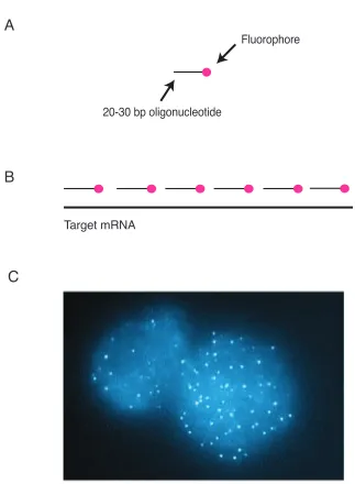
Single molecule FISH techniques work through a tiling approach where multiple

complementary oligonucleotide probes, each coupled to a fluorescent dye, are used

to mark individual RNA transcripts in situ [14, 91]. (Figure 2.1). In this technique,

each oligonucleotide is approximately 30 bases long, and as a 30-mer, it can have

many instances of non-specific binding throughout the transcriptome. However, each

oligonucleotide will have di↵erent non-specific targets, and since we use multiple

oligos in each probe, only the real RNA target will be bound by every oligonucleotide,

producing bright spots with excellent signal to noise. With single molecule FISH,

individual RNA transcripts are easily quantified as distinct fluorescent spots, and

with image processing, the spots can be counted for a direct measurement of gene

expression.

(23)

Target mRNA

Fluorophore

20-30 bp oligonucleotide

A

B

C

(24)

paternal transcripts are nearly identical, save for the occasional heterozygous SNPs. In

order to classify these transcripts as maternal or paternal, we must be able to reliably

distinguish a single SNP. Larsson et al.[92] have described one such technique for doing

so through rolling circle amplification. A key limitation of rolling circle amplification

is the series of enzymatic reactions required to perform it. These enzymatic steps can

introduce significant variability to results, as slight di↵erences in enzyme efficiency

can propagate into highly divergent results. In Larsson’s work, only about 1% of

transcripts are detected, rendering interpretation difficult. Moreover, enzymatic steps

often require longer incubation times and higher costs, so an ideal technique would

provide high detection efficiencies without the use of enzymes.

In this section, we will describe SNP-FISH, a technique that enables single-cell allele

specific expression in situ without the aid of enzymes. Instead, SNP-FISH borrows

from advances in directed DNA binding to create a SNP detection probe that can

distinguish a SNP based on a toehold exchange reaction [93, 94]. In this chapter,

we will extensively model and test SNP-FISH in order to understand its operating

(25)

2.2 Materials and Methods

2.2.1 SNP-FISH Method Rationale

In order to adapt standard single molecule FISH, we must solve a series of specificity

problems. The first and most obvious is to create a RNA probe that can reliably

distinguish a di↵erence as subtle as a single DNA base pair. With a 30 base long

oligonucleotide, a single base pair mismatch does little to discourage promiscuous

binding to both alleles. However, if shorter oligonucleotides are used, then the base pair

mismatch contributes more significantly to the binding affinity of the oligonucleotide,

leading to proper discrimination between the two alleles. In order to achieve this

specificity, an oligonucleotide would have to be approximately 8 base pairs long, but

this is highly problematic because an 8 base pair long oligonucleotide would have

tremendous non-specific binding throughout the transcriptome. Moreover, an eight

base long oligonucleotide would not bind very stably due to its short length, and thus

might not survive the typical washes in the SNP-FISH protocol.

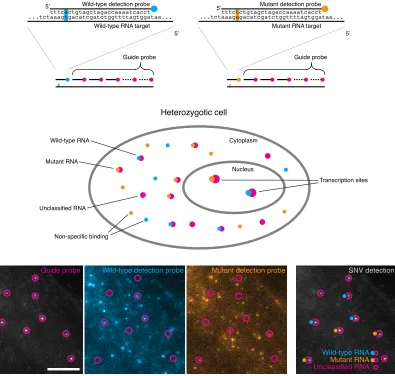
In order to overcome these problems, we designed special SNP detection

oligonu-cleotides inspired by the specificity achieved in in vitro DNA strand displacement

reactions[93, 94]. The probes are comprised of standard 28-32 base pair long

oligonu-cleotides attached to one of two fluorescent dyes, one for each allele. In order to achieve

specificity, we mask the detection probe with a complementary oligonucleotide, leaving

a 7- 10 base pair overhang called the toehold, illustrated in Figure 2.2. The SNP is

located in the middle of the toehold, at the 5th position from the five prime end, and

with most of the probe masked, it is sufficiently destabilizing to promote allele specific

(26)

intermediate conformation, and then undergoes a strand displacement reaction where

the mask peels o↵ and the oligonucleotide fully binds to the RNA target. The final

state of having the probe fully bound to the target with free-floating mask is the most

thermodynamically favorable, driving the reaction forward [93, 94].

With this approach, the SNP oligonucleotides will not cross-hybridize, giving us the

ability to discriminate between a single base pair di↵erence, but there remains another

specificity challenge. Since they are comprised of only one oligonucleotide, these SNP

probes will bind to many other random targets in a cell’s transcriptome and we are only

interested in the binding events that occur on a given gene of interest. We can solve this

challenge by leveraging the spatial information in our assay. Specifically, we can design

a conventional single molecule FISH probe, consisting of multiple oligonucleotides, and

use this probe to accurately locate the desired RNA molecule. We can then perform a

colocalization analysis between this “guide” probe and the SNP detection fluorescent

channels. If a SNP detection probe occurs in the same spot as the guide probe, then

we assume that they are bound to the same molecule and we can therefore classify

that RNA as coming from that allele. Not all guides will necessarily have a SNP probe

that colocalizes, so those transcripts remain undetected. The approach is illustrated in

Figure 2.3. It is possible to have a guide spot colocalize with a probe in both channels.

These“three-color” spots are typically thrown out of the analysis as they are thought to

be autoflourescent debris or otherwise uninterpretable. In later experiments, however,

when probing multiple SNPs simultaneously, these three-color spots will become more

(27)

Wild-type detection probe

Wild-type RNA target

Initial binding

Stabilization

gtagctagaccaaaatcacct

aaagtgacatcgatctggttttagtggataa...

aaagtgacatcgatctggttttagtggataa... ...tct ...tct Mask oligonucleotide gatctggttttagtgga Mask oligonucleotide gatctggttttagtgga tttcact

agctagaccaaaatcacct tttcactgt

tttcactgtag

Mutant detection probe

Mutant RNA target

aaagagacatcgatctggttttagtggataa...

Mutant RNA target

aaagagacatcgatctggttttagtggataa... ...tct

...tct tttctct

agctagaccaaaatcacct tttctctgt

tttctctgtag No cross hybridization

ctagaccaaaatcacct

gatctggttttagtgga ctagaccaaaatcacctgatctggttttagtgga

(28)

Unclassified RNA Wild-type RNA

Mutant RNA

Guide probe Wild-type detection probe

aaagtgacatcgatctggttttagtggataa... ...tct

Guide probe

Non-specific binding Unclassified RNA

Transcription sites

Heterozygotic cell

Wild-type RNA

Mutant RNA

Cytoplasm

Nucleus Wild-type detection probe

Mutant RNA target

aaagagacatcgatctggttttagtggataa... ...tct

Guide probe Mutant detection probe

Mutant detection probe SNV detection

(29)

2.2.2 Cell culture and fixation

To validate SNP-FISH, we grew human melanoma cell lines with the BRAF V600E

mutation, SK-MEL-28 (Mut/Mut, ATCC cat no HTB-72), WM3918 (WT/WT) and

WM398b & WM9 (both WT/Mut) (gifts from the lab of Meenhard Herlyn, Wistar

Institute, genotypes verified by the Herlyn lab), using the recommended cell culture

guidelines for each line. We obtained GM12878 cells from the Coriell Cell Repositories

and grew them according to standard guidelines. Mouse embryonic fibroblasts (MEF)

were isolated at embryonic day 13.5 as described in Verona et. al 2008[95]. MEFs

were obtained either from C57BL/6 (B6) mice crossed with B6 mice, or B6 mice

crossed with CAST/Eij (CAST7) strain (C7)[96], which possesses chromosome 7 from

the Mus musculus castaneus strain in a C57BL/6 (B6; The Jackson Laboratory, Bar

Harbor, ME) background. We grew MEFs in DMEM with GlutaMax (Gibco) with 10%

FBS (Sigma) and penicillin/streptomycin. We grew the cells on Lab-Tek chambered

coverglass (Lab-Tek) and fixed the cells following the protocol in Raj et al. Nat Meth

2008[14].

2.2.3 Probe design and synthesis

We designed detection probes with the single nucleotide di↵erence located at the

5th base position from the 5’ end. We adjusted the total length of the detection

oligonucleotide to ensure the hybridization energy with target RNA was similar or

greater than that of the guide probe oligonucleotide[94]. We designed mask

oligonu-cleotides complementary to the detection probes that, upon binding to the detection

probe, left a 6 to 11 base toehold regions available to target RNAs regions with SNPs.

Probe design software, written in Python, is available through the Raj lab bitbucket

(30)

guide probe oligonucleotides to ATTO 488 dye (ATTO-TEC), ATTO 700, or CalFluor

610 (Biosearch), and we interchangeably used Cy3 and Cy5 (GE Healthcare) dyes

for the SNP detection probes. We did not observe any changes to detection efficiency

when swapping the Cy3/Cy5 dyes. Dyes were chosen to be chemically similar to each

other in order to minimize the dye-specific affinity di↵erences of the detection probes.

2.2.4 Allele Specific RNA FISH

We performed RNA fluorescence in situ hybridization (FISH) as outlined in Raj et

al. Nat Meth 2008[14] with some modifications as outlined presently, most notably

a postfixation step after the hybridization to help prevent probe dissociation during

imaging. Firstly, our hybridization bu↵er consisted of 10% dextran sulfate, 2x

saline-sodium citrate (SSC) and 10% formamide[23]. We performed the hybridization using

final concentrations of 5nM for the guide probe, wild-type and mutant detection probe,

and 10nM for the mask, thereby leading to 1:1 mask:detection oligonucleotide ratios.

We let the hybridization proceed overnight at 37C. For Lab-Tek chamber samples, we

used 50µL hybridization solution with a coverslip and included a moistened paper

towel to prevent excessive evaporation in parafilmed culture dish. For suspension cells,

we used 50µL hybridization solution in a 1.5mL Eppendorf tube. In the morning, we

washed the samples twice with a 2X SSC and 10% formamide wash bu↵er. Suspension

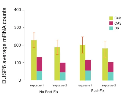
cells included 0.1% Triton-X in the wash bu↵er. We then performed a postfixation step

using 4% formaldehyde in 2X SSC for 30 minutes at 25C to crosslink the detection

probes and thereby prevent dissociation during imaging, followed by 2 washes in 2X

SSC. We then put the cells into anti-fade bu↵er with catalase and glucose oxidase[14]

(31)

step on SNP-FISH. While we observed qualitative di↵erences between samples in the

photobleaching patterns of repeated exposures between samples that were postfixed

and those that were not, we did not see significant di↵erences in detection efficiency,

shown in Figure 2.4. We subsequently omitted the post-fixation step for the MEF

experiments.

2.2.5 Imaging and image analysis

We took all our images on a Leica DMI600B automated widefield fluorescence

microscope equipped with a 100x Plan Apo objective, a Pixis 1024BR cooled CCD

camera and a Prior Lumen 220 light source. We took image stacks in each fluorescence

channel consisting of sets of images separated by 0.35µm. Our exposure times were

1500ms for atto 488 guide probes, 2000 for CalFlour610 guide probes, and 3500ms for

Cy3/Cy5 SNP detection probes. We used longer exposure times for the wild-type and

mutant detection probes owing to the low signal produced by single dye molecules

relative to the dozens of fluorophores typically used in the guide probes.

We first segmented and thresholded images using a custom MATLAB software suite

(downloadable at https://bitbucket.org/arjunrajlaboratory/rajlabimagetools/wiki/Home).

Segmentation of cells includes the nuclear and cytoplasmic region. We fit each spot

to a two-dimensional Gaussian profile specifically on the z-plane that it occurs in

order to ascertain sub-pixel resolution spot locations as well as intensity amplitudes.

Colocalization took place in two stages; in the first stage, guide spots searched for the

nearest neighbor SNP probes within a 3.0 pixel (360 nm) window. We ascertained the

median displacement vector field for each match and subsequently used it to correct

for chromatic aberrations. After this correction, we used a more stringent 1.5 (195 nm)

(32)

(33)

for a more detailed discussion on the colocalization radius.

2.2.6 Statistical analysis of allele specific expression

We performed a statistical analysis of allele specific expression in two stages. See

the results section for the mathematical derivation and justification for this approach.

In the first stage, we combined data from all cells to find evidence for population-level

allelic imbalance. Using this data, we computed the mean detection efficiency of

the detection probes as well as the average percentage of detected transcripts that

originated from the maternal or paternal allele of the gene in question. We computed

confidence intervals on these percentages by combining a. the error associated with the

number of observations itself (modeled as a multinomial distribution and computed to

95% confidence) and b. the error associated with uncertainty in the detection efficiency.

For the latter, we assumed that the detection efficiency could di↵er by at most 8% from

each other; for example, if the average detection efficiency was 55%, we would compute

the imbalance with 59%/51% detection efficiencies, first in favor of maternal and then

paternal. Empirically, we have found that our detection efficiencies tend to remain in

the 50%-60% range, and so this procedure will ensure that at least one of the detection

efficiencies remains in this range. Combining these two sources of error, our error bars

likely reflect a greater than 95% confidence interval. In the next stage, we used the

observed detection efficiency and population-level imbalance to ascertain the degree

to which single cells displayed allelic imbalance. Our null hypothesis is that each RNA

produced at any given period of time would be independently chosen to come from

either the maternal or paternal allele at the same frequency as at the population level;

in other words, there are no “runs of maternal or paternal-origin transcripts in single

(34)

observed imbalances for each cell given the population-level imbalance. We used these

densities to compute single cell likelihoods for our observed counts and calculated the

total likelihood of the population by taking the product of the single cell likelihoods.

We then compared the likelihood of our observations to the likelihood one might expect

from the null hypothesis by generating 1,000,000 in silico counts for each cell based on

our multinomial model and computing the likelihood of these observations to generate

a distribution of likelihoods corresponding to the null hypothesis. In order to reject

the null hypothesis and show that the population of single cells displays cell-to-cell

allelic imbalance, we then computed the percentage of the null hypothesis likelihoods

(35)

2.3 Results and Discussion

2.3.1 SNP-FISH proof of concept

Using a set of melanoma lines, we established proof of concept with SNP probes

designed to the V600E mutation, a key mutation in cancer resistance[97]. Specifically,

we used a wild-type homozygous line, mutant homozygous line, and two di↵erent

heterozygous lines to test SNP-FISH. As shown in Figure 2.5, we observed that the

wild-type cells were predominantly detected as wild type, with 58% of guide spots

colocalizing with wild-type SNP probe and 7% colocalizing with the mutant SNP

probe. The homozygous mutant cells were predominantly detected as mutant, with

56% of guide spots colocalizing with the mutant probe and 7% colocalizing with the

wild-type probe. Guide spots in the heterozygous cells showed approximately equal

counts of wild-type and mutant SNP probes colocalizing (33% for wild type and 34%

for mutant).

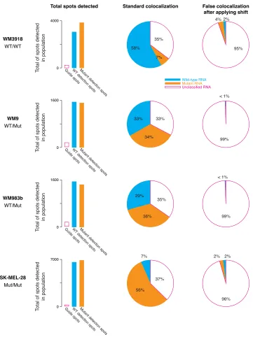
Looking more closely at the two homozygous lines, we observed some degree of

false positives (about 7%). To test whether these false positives are due to random

colocalization with spurious pixels or whether they were indeed real cross-hybridization

events, we performed pixel shift control, where the guide RNA’s positions were

trans-lated by adding 8 pixels to the x and y coordinates, and colocalization was performed

again. This allows the guide spots to experience a similar ’background’ environment

in terms of non-specific binding, while ablating the real signal. If the false positive

rate stays the same after pixel-shifting, then it is due to spurious colocalization. If it

drops, then it is due to a real detection event. As shown in Figure 2.6, the detection

(36)

Unclassified RNA

Wild-type RNA

Mutant RNA

Guide probe Wild-type detection probe

Figure 1

Initial binding Stabilization 5’ 5’ 5’ gtagctagaccaaaatcacct aaagtgacatcgatctggttttagtggataa...

Wild-type RNA target 5’ aaagtgacatcgatctggttttagtggataa... ...tct ...tct Mask oligonucleotide gatctggttttagtgga Mask oligonucleotide gatctggttttagtgga Guide probe Non-specific binding Unclassified RNA 0 WM3918

Number of BRAF mRNA

per cell

WT/WT WT/Mut Mut/Mut

WM9 WM983b SK-MEL-28

40 Transcription sites Heterozygotic cell Wild-type RNA Mutant RNA Cytoplasm Nucleus tttcact

Wild-type detection probe 5’

5’

tttcactgtag

Mutant RNA target 5’

5’ 5’

aaagagacatcgatctggttttagtggataa...

Mutant RNA target 5’ aaagagacatcgatctggttttagtggataa... ...tct ...tct Guide probe tttctct

Mutant detection probe 5’

5’

tttctctgtag

No cross hybridization

5’

ctagaccaaaatcacct gatctggttttagtgga

Mutant detection probe SNV detection

0 15 30 0 10 20 0 10 20 Unclassified RNA Wild-type RNA Mutant RNA 5’ ctagaccaaaatcacct gatctggttttagtgga 8 2 7 7 12 4 4 7 4 3 4 Heterozygotic cell

Individual cells Individual cells Individual cells Individual cells

Figure 2.5: SNP FISH detects allele specific expression of the BRAF V600E mutation. Each bar represents individual cells. Wild-type cells are detected as mostly wild type (left). Mutant cells are detected as mostly mutant (right). Heterozygous cells show both wild-type and mutant detection. Overall detection efficiency is approximately 65%.

suggests that of the 7% false positives, roughly half are real cross-hybridization events

and half are due to spurious colocalization arising from the high density of the SNP

probes. This is in contrast to the heterozygous lines, which have fewer wild-type and

(37)

Supplementary Figure 2

Supplementary Fig. 2. Measurement of false positive rates due to random colocalization. Bar graphs show

the number of guide spots and detection spots identified in all the cells we analyzed. The pie charts show the degree of colocalization in the original images (left) and after applying a 8 pixel shift in x and y to the detection spots (right). The latter serves as an estimate of how often spots would be likely to colocalize purely by chance. We found that these rates of colocalization were very low, with the vast majority of spots remaining unclassified after applying the shift.

Unclassified RNA Wild-type RNA Mutant RNA < 1% 99% 29% 36% 35% 0 WM983b WT/Mut 1600 T

otal of spots detected

in population

Guide spotsWT detection spots

Mutant detection spots

2% 2% 96% 56% 37% 0 SK-MEL-28 Mut/Mut 7000 T

in population

Guide spotsWT

detection spotsMutant detection spots 0

WM3918

Standard colocalization

Total spots detected False colocalization after applying shift

WT/WT

4000

T

in population

Guide spotsWT

detection spotsMutant detection spots

2% 4% 95% 58% 7% 35% 0 WM9 WT/Mut 1600

Total of spots detected

in population

Guide spotsWT detection spots

Mutant detection spots

< 1% 99% 33% 34% 33% 7%

(38)

2.3.2 Formulation of statistical framework for analysis

In this section, we will develop the mathematical and statistical framework for

understanding SNP-FISH and its implications for interpreting experimental results.

Allelic imbalance model

Consider a population of cells expressing a gene of interest with di↵erent maternal

and paternal alleles. After an in situ experiment, we count a total number of mRNA

T expressed over a population of N cells, observing some fraction of them labeled

maternally Om, and paternally,Op, and some fraction undetected,U.

Modeling imbalance

We can model imbalance by the parameter Im (range 0-1), which tells us the

prob-ability that a given mRNA molecule was transcribed from the maternal chromosome

(or any reference chromosome in general as Ip = 1 Im. The null hypothesis in this

situation is balanced expression. In other words, an mRNA transcript is equally likely

to have come from either the paternal or maternal allele (Im = 0.5). Given a total

count of RNAT, the number of transcripts originating from the maternal chromosome,

Tm is modeled by a binomial distribution with parameters T and Im. This model

assumes independence between every transcript.

Modeling detection efficiency

(39)

force, and cell type. Ideally, detection efficiency does not change for a given allele in

a given cell, but we will consider a model that can account for di↵erent detection

efficiencies for the di↵erent alleles in order to provide robust confidence bounds.

An mRNA has probability dm of being detected if it is maternal and dp if it is

paternal. We expect, based on empirical evidence, that dm and dp range between

0.50-0.60 and are within 10% of each other. The number of detected mRNAs will

also be binomially distributed with respect to the total number of mRNA, as we

assume that the probability of detection is independent and equal for each transcript.

Indeed, we can look at the variability of detection efficiency in single cells to check for

systematic errors that might be a↵ecting the results.

Performing simulated detection experiments

In order to simulate detection experiments, and define a null, we must findP(Om =

m, Op = p|T). Let Tm and Tp be random variables representing the true count of

mRNA from the maternal and paternal allele respectively (note thatTm+Tp =T).

P(Om =m, Op =p|T) = X

Tm

P(Om =m, Op =p|Tm, T)P(Tm =n|T)

Given Tm, Om, andOp are just drawn from a joint binomial distribution.

P(Om =m, Op =p|Tm, T) = ✓

Tm

m

◆

dm_m(1 dm)Tm m ✓

T Tm

p

◆

dp_p(1 dp)T Tm p

Based on our allelic imbalance model, P(Tm =n|T) is binomial with parameters

T and Im. Thus, the simulated experiment pdf is the sum of the product of three

(40)

P(Om =m, Op =p|T) = X

Tm

bino(Tm, dm)bino(T Tm, dp)bino(T, I)

P(Om =m, Op =p|T) = T X

n=0

✓

n m

◆

dm_m(1 dm)Tm m ✓

T n

p

◆

dp_p(1 dp)T Tm p ✓

T n

◆

I_mn(1 Im)T n

Alternatively, we can express P(Om =m, Op = p|T) as a multinomial distribution.

Consider an individual mRNA r. The probability that it will be observed coming from

the maternal allele is the equal to the probability that it came from the maternal

allele times the probability of maternal detection.

P(r₂Om) =P(r2Om|r 2Tm)P(r 2Tm)

P(r ₂Om) = dmIm =↵

Analogously, we have:

P(r 2Op) = dp(1 Im) =

If r is not observed as maternal or paternal, then it is undetected, thus:

P(r ₂U) = 1 dp(1 Im) dmIm =

Thus, we can generate our experiments in a more computationally efficient manner

(41)

P(Om =m, Op =p|T) =

T!

m!p!(T m p)!↵

m p T m p

Population level parameter estimation

When estimating parameters for a cell population, the ideal case is when both

probes have the exact same binding affinity and therefore detection efficiency. However,

probes could have biases in detection efficiency, so we must extend the ideal case in

order to understand whether an imbalance is due to probe detection di↵erences as

opposed to actual di↵erences in RNA abundance.

Equal detection efficiencies When dm =dp = d exactly, it is very easy to find

the maximum likelihood estimate of Im for a given experiment givenOm,Op, and T.

Om

Om+Op

= ↵M LE ↵M LE + M LE

= (dIm)M LE

(dI)M LE + (d(1 Im))M LE

In this situation, detection efficiency and imbalance are independent given the

total RNA detected Om+Op, thus:

(dIm)M LE

(dI)M LE+ (d(1 Im))M LE

= dM LEImM LE

dM LEImM LE +dM LE(1 ImM LE)

=ImM LE

Thus, for a given experiment, we estimate our parameters by: (note that ˆx= xM LE)

ˆ

I = Om Om+Op

ˆ

(42)

We can generate confidence intervals by (1) a Monte Carlo approach where we

use the estimated parameters to generate 100,000 experiments and re-estimate the

parameters for each experiment to obtain an empirical distribution for ˆI and ˆd.

Alternatively (2), we can calculate the explicit probability mass function (PMF) of

ˆ

I by calculating ˆI =f(Om, Op) at every possible value of Om andOp, and summing

over those values accordingly with their associated probabilities as given byP(Om =

m, Op =p|T) = _m_!_p_!(_{T m p}T! _)!↵m p T m p.

Unequal detection efficiencies With unequal detection efficiencies, we are not so

lucky as to have a simple way of fitting ˆI from Om and Op. When we have measured

dm and dp with two separate experiments in cells that are homozygous wild type and

homozygous mutant, we want to find the Im that maximizes:

P(Om =m, Op =p|T) =

T!

m!p!(T m p)!(dIm)

m₍_d

p(1 Im))p(1 dp(1 Im) dmIm)T m p)

The maximum occurs at _@_I@_mP(Om =m, Op =p|T) = 0 = _@_I@_mlnP(Om = m, Op =

p|T).

0 = @ @Im

ln⇥(dmIm)m(dp(1 Im))p(1 dp(1 Im) dmIm)T m p ⇤

0 = @ @Im

[mln(dmIm) +pln(dp(1 Im)) + (T m p) ln((dp dm)Im+ 1 dp)]

0 = mdm dmIm

pdp

dp(1 Im)

+(T m p)(dp dm) (dp dm)Im+ 1 dp

(43)

0 = Om Im

Op

(1 Im)

+ U a

aIm+b

0 =Om(1 Im)(aIm+b) OpIm(aIm+b) +U aIm(1 Im)

0 =Om(aIm+b aIm2 bIm) Op(aIm2 +bIm) +U(aIm aIm2)

0 =OmaIm+Omb OmaIm2 OmbIm OpaIm2 OpbIm+U aIm U aIm2

0 = a(Om+U+Op)Im2 + (Oma Opb Omb+U a)Im+Omb

0 = aT I_m2 + ((U +Om)a (Om+Op)b)Im+Omb

Thus,

ˆ

I(Om, Op, U, dm, dp) =

(U a (Om+Op)b)± p

((U+Om)a (Om+Op)b)2 4( aT)(Omb)

2aT

The physically realizable solution will be the root that falls along the interval [0,1],

which will be the minus solution.

For the experiments where we only take measurements from a heterozygous

popu-lation, such as in GM12878, we do nota priori know the di↵erent detection efficiencies.

However, using our best empirical guess, we assume that the MLE of the detection

efficiencies is whendm =dp =dobs where dobs = Om_T+Op. In reality, it is possible that

there is some di↵erence between the maternal and paternal detection efficiencies, but

we do not expect this di↵erence to be more than 8% based on our empirical data.

To compute confidence intervals, we take the two extreme cases where the detection

efficiencies di↵er by 8%, one will lead to an upper bound MLE of ˆI and one will lead

to a lower bound estimate.

(44)

• dm2 =dobs 0.04 anddp2 = 1.05dobs+ 0.04

Based on those above two cases, we calculate ˆIU B and ˆILB as shown above. We

independently generate 95% confidence intervals for both cases of parameters via

Monte Carlo simulation. Our true confidence interval is then the maximum of the 95%

confidence interval of ˆIU B and the minimum of the 95% confidence interval of ˆILB.

Single-cell imbalance analysis

Once we have determined the overall population level parameters, we can then ask

if the cells are behaving as consistent subsets of the population. In other words, do the

parameters that best fit the population do a good job of fitting all of the single cells.

To answer this question, we assume a null hypothesis that the cells are independent,

governed by the same parameters that best fit the population. In other words, if the

population imbalance is 50-50, we expect each cell to be 50-50 as well, as opposed to

50% of cells expressing 100% of one allele and the other 50% expressing 100% of the

other allele.

To quantify this, we take our population level parameters, ˆI, ˆdm, and ˆdp. For each

of the N cells, we know the total number of mRNA in the cell Tn, and how many

were observed as maternal, Omn and paternal Opn. We can consider each cell as an

independent experiment, and in doing so, can calculate the range of imbalances that we

would expect to see in that cell given the population level parameters. Specifically, we

compute the exact PMF for ˆIn for each of the N cells as explained above. From these,

we compute a likelihood of the total experiment multiplying together the probabilities

(45)

In order to obtain a p-value on the observed likelihood, we use Monte Carlo

to sample the imbalance PMFs of the N cells, and using these simulated per cell

imbalances, we generate an empirical distribution of expected likelihoods for the total

experiment- in other words, our null distribution. To compare these, we plot the

ln`obs to see where it falls along the negative log of the likelihood distribution for

simulated experiments. We can interpret the - log likelihood distribution as a one-sided

test where the p-value is the the probability that the log likelihood distribution would

generate a likelihood greater than the observed likelihood. In other words,

p-value =P { lnlobs > ln`dist}

Applications to allelic imbalance in human genes

Armed with this statistical framework, we explored allelic imbalance in human

genes. We chose the deeply sequenced Tier I encode cell line[98], GM12878, as phased

diploid genome sequences were readily available [41]. Moreover, this cell line has

been commonly used in many studies analyzing allele specific expression with

high-throughput techniques [41, 65, 99, 100].

We chose three genes,DNMT1,EBF1, andSUZ12, for which we found heterozygous

SNPs in the GM12878 line. Using these genes, we quantified the population level

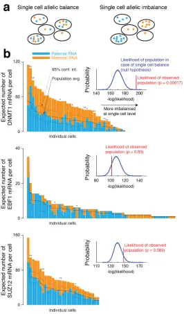
imbalance as defined above, shown in Figure 2.7. DNMT1 did not exhibit statistically

significant allelic imbalance at the population level, while EBF1 exhibited significant

paternal bias and SUZ12 exhibited mild paternal bias. Consistent with these findings,

EBF1 has been previously identified as a gene exhibiting allelic imbalance [38].

After looking at the population level statistics, we looked to see whether there was

(46)

0.0 1.0

0.5

Allelic imbalance in

cell population

Maternal

95% confidence interval Paternal

DNMT1

EBF1

SUZ12

(47)

level, single cells could either exhibit balanced expression where every cell is essentially

identical to every other cell, reflecting the population average, or cells could be highly

variable, with some cells expressing all of only one allele and others expressing all of

the other, in a salt and pepper pattern.

We analyzed where along this spectrum lay the single-cell imbalances for DNMT1,

EBF1, and SUZ12 in Figure 2.8. DNMT1, though balanced at the population level,

exhibited significant single cell imbalance (p = 0.00017), while EBF1 and SUZ12,

though both exhibited imbalanced expression at the population level, exhibited no

evidence of single cell imbalance.

Of note, the ability to detect imbalances at the single-cell level is robust to significant

variability in experimental parameters, as illustrated in Figure 2.9. Specifically, we

wondered whether di↵erences in probe binding affinity could manufacture a spurious

imbalance at the single-cell level. We found, however, that even very large changes in

(48)

Figure 3.10: a. Diagram of single cell allelic balance and imbalance. b. Allelic imbalance in single cells. The solid black midline represents the average imbalance across cells (from a). The dashed black lines shows the 95% confidence interval on the imbalance for each cell with the null hypothesis that the probability of an RNA being maternal or paternal is independent of which cell it is in. The inset shows the likelihood of the observed population imbalance (red) compared to that of the null model (blue); see methods for details. Note that for EBF1, 90% of cells expressed zero transcripts, so we excluded those cells from the figure. Each sample shown is one of a set of at least two biological replicates. ** represents cells with a p-value below 0.05, and * represents a p-value

(49)

a

b

Degree of imbalance

Assuming equal detection efficiency

Assuming paternal detection efficiency of 0.35

Assuming paternal detection efficiency of 0.75

Total number of RNA

detected

0.55

40% detection efficiency 50% 60% 70% 0 200 400 0.70 0.85 Probability

Likelihood of observed population (p = 0.00017)

-log(likelihood)

More imbalanced at single cell level

140 160 180 200

-log(likelihood)

160 180 200 220

-log(likelihood)

160 180 200 220

Likelihood of population in case of single cell balance (null hypothesis)

Likelihood of observed population (p = 0.000069) Likelihood of observed

population (p = 0.00017)

-log(likelihood)

110 130 150 170

-log(likelihood)

110 130 150 170

Probability

-log(likelihood)

80 100 120 140

Probability

-log(likelihood)

110 130 150 170

-log(likelihood)

120 140 160 180

-log(likelihood)

130 150 170 190

Supplementary Figure 5

Supplementary Fig. 5. a. Using a statistical model, we determined the number of RNAs required to say

whether there was an allelic imbalance (for a given actual degree of imbalance). This number is relatively insensitive to the detection efficiency. b. We examined the degree to which changes in the detection efficiency between maternal and paternal detection probes would affect the determination of the presence of single cell imbalance. We found that even very large changes in the detection efficiencies would qualitatively similar conclusions. This is because single cell imbalance manifests as a deviation from the average, thereby making it insensitive to parameters governing the determination of the average itself.

DNMT1

EBF1

SUZ12

(50)

2.3.3 Exploring and optimizing parameter space

Having established SNP-FISH and its analytical foundation, we will now explore

and optimize more of the parameters that a↵ect SNP-FISH. In this section, we will

describe general heuristics and design principles with supporting data. We emphasize

that SNP-FISH requires some degree of specialized optimization for every target. We

have found that targeting some SNPs works very well (detection efficiency >50%) and

other SNPs work very poorly (detection efficiency<20%). While we cannot currently

predicta priori whether a SNP-FISH probe will work, the principles that we describe

here can serve as instructive examples for future optimization.

Importance of the oligonucleotide mask

Another demonstration of allele specific single molecule FISH was published

con-currently with SNP-FISH by Hansen et. al [101]. In their work, they looked at allele

specific expression ofNanog in a divergent mouse cross that was replete with multiple

SNPs. They achieved allele specific signal with oligonucleotide probe sets that targeted

at least 12 SNPs simultaneously, without the use of a mask. Using just one SNP

probe with BRAF, however, we found that the mask was necessary for proper SNP

discrimination. Without the mask, the wild-type melanoma line appeared

heterozy-gous due to the significant increase of non-specific binding, as shown in Figure 2.10.

One can conclude that if many SNPs are available, then their cumulative e↵ect can

confer sufficient specificity as to make the mask dispensable, but in cases where only

(51)

0

WM3918

Number of BRAF mRNA

per cell

WT/WT

40

Mask No mask

Figure 2.10: Allele specific BRAF expression in the presence and absence of a mask oligonucleotide. With the mask, the SNP-FISH assay correctly detects the wild-type allele, but without the mask, the assay loses its specificity and both SNP probes bind promiscuously.

thereby the length of the toehold overhang). With BRAF, we found that increasing

the mask length from a range of 7 to 11 nucleotides could increase the detection

efficiency without significantly a↵ecting false positive rates, as shown in Figure 2.11.

With other genes, we have observed that varying the mask length over this range can

improve detection efficiency by a moderate amount (approximatley 10%). We consider

a SNP probe to be good if the detection efficiency is>50%. In general, if a SNP probe

exhibits very low detection efficiency (<15%), changing the mask length will not bring

(52)

Figure 3.7: Changing the toehold length can change the detection efficiency without dramatically increasing off-target binding. Toehold length is in nucleotides, with the total probe length remaining constant (toehold length changed by changing the mask probe length). With no mask there is dramatically reduced target discrimination and overall detection efficiency saturates around 67%. We computed the free energy change of the toehold binding (given in kcal/mol) using the definition from [87]

Figure 2.11: E↵ect of varying mask length on detection efficiency. With no mask, there is no allele specific discrimination, but varying the mask length can improve the detection efficiency without increasing cross-hybridization

(53)

Tuning the colocalization radius

When performing colocalization between the guide channel and the SNP channels,

one must determine the allowable distance between two spots in order to determine

a match. Super-resolution imaging techniques have proved that these images are

extremely precise[102], however there are still many factors that one needs to account

for, most prominently chromatic aberration [103]. Our colocalization analysis algorithm

performs a first order correction for shifts between fluorescent channels by performing

colocalization in two rounds. The first round is a permissive round where a larger

colocalization radius is used. After this round, the median displacement vector is

computed between two fluorescent channels and is used to shift correct positions for a

second, more stringent, round of colocalization.

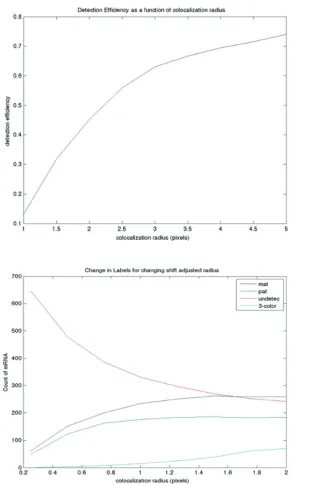
We explore the e↵ects of colocalization radius for the DNMT1 gene in Figure

2.12. For the initial colocalization step, we see that detection efficiency increases

rapidly with increasing radius, up to about 3 pixels, after which point it begins to

increase more gradually, suggesting that additional colocalization events are likely

due to nonspecific background spots. For the shift-corrected colocalization, we see an

optimum at approximately 1 pixel, beyond which the rate of three-color spots begins

to rise significantly. In our imaging setup, one pixel is 130 nm in length, which means

that the first round of colocalization should search for RNA spots less than 325 nm to

ascertain the shift correction, and then within 130 nm after shift correcting. Of note,

since the length of a DNA base pair is approximately 0.34 nm and typical transcript

targets are often on the order of kilobases, these colocalization radii are consistent

with the distances we might expect. These results are valid for DNMT1, but may

(54)

Visualizing Allele Specific Expression In Single Cells

University of Pennsylvania

ScholarlyCommons

Visualizing Allele Specific Expression In Single

Cells

Paul Ginart

Visualizing Allele Specific Expression In Single Cells

Contents

List of Figures

Chapter 1

Introduction

1.1

Taking inventory: genes and measuring gene

expression

1.2

There’s more than one of everything: allele

specific gene expression

1.3

The teeming hidden world: single cell

variabil-ity

1.4

More than your genes: epigenetics and

ge-nomic imprinting

1.5

Thesis Overview

Chapter 2

SNP-FISH: visualizing allele

specific expression in single cells

2.1

Introduction

A

B

C

2.2

Materials and Methods

2.2.1

SNP-FISH Method Rationale

2.2.2

Cell culture and fixation

2.2.3

Probe design and synthesis

2.2.4

Allele Specific RNA FISH

2.2.5

Imaging and image analysis

2.2.6

Statistical analysis of allele specific expression

2.3

Results and Discussion

2.3.1

SNP-FISH proof of concept

Figure 1

2.3.2

Formulation of statistical framework for analysis

Allelic imbalance in

cell population

DNMT1

EBF1

SUZ12

a

b

Supplementary Figure 5

2.3.3

Exploring and optimizing parameter space