22 & 23.04.2017
In association with
I
nternational
Journal
of
Scientific
Research in
Science and
Technology
Performance analysis of optimally tuned 2DOF-PID controller for
Automatic Load Frequency Control
Nivedita G R
*1, Kamaraj N
2*1Electrical and Electronics Engineering, Thiagarajar College of Engineering, Madurai, Tamil Nadu, India [email protected]
2
Electrical and Electronics Engineering, Thiagarajar College of Engineering, Madurai, Tamil Nadu, India [email protected]
ABSTRACT
In a Power system, if the load varies the frequency of the generator also varies. Automatic load frequency control plays a major role in maintaining the frequency constant. Various controllers like PI, PID and 2DOF-PID are used for controlling the load frequency in power system. Two degree of Freedom Controller optimized by Particle Swarm Optimization will help to adjust the generator frequency to ensure stable and efficient response due to sudden changes in load. The single area power system consisting of non-reheat thermal power plants with 2DOF-PID controller has been considered for design and analysis. The gains of the 2DOF-PIDcontroller is optimized by the particle swarm optimization to have a better dynamic performance, to reject the load disturbance , to improve the robustness and also to reduce the Integral Time Absolute Error which is caused due to sudden changes in load demand.
Keywords:Automatic load frequency control; Transient stability; Two Degree of freedom; Particle Swarm Optimization; Dynamic performance; parameter uncertainties; performance index; steady state error; Integral time absolute error
Abbreviations and Acronyms: Kt-turbine gain; Tt-Turbine time constant; Kg-Governor gain; Tg- Governor time constant; Kps-power system gain; Tps-Power system time constant; R-Governor speed regulation; B-frequency Bias parameter T1-synchronising coefficent;Kp-Proportional gain; Ki-Integral gain; Kd- Derivative gain; ITAE-Integral Time Absolute Error;2DOF -two degree of freedom
I.
INTRODUCTION
In an interconnected electrical power system both the voltage and frequency to be fixed at desired values irrespective of change in loads that occurs randomly. To cancel the effect of load variation and to keep the frequency constant a control system is required. Though the active and reactive powers have a combined effect on the frequency and voltage, the control problem of the frequency and voltage can be separated. Frequency is mostly dependent on the active power. The active power and frequency control is called as load frequency control (LFC). Themost important task of LFC is to maintain the frequency constant against the varying active power loads. The main purpose of LFC system are to keep in zero steady state error in frequency deviation for single
area system, optimal transient performance and to have reduced oscillation in the system due to frequent change in load demand. The gains of the controller can be optimized by the modern heuristic algorithm (PSO-Particle Swarm Optimization) and also to reduce theperformance index Integral Time Absolute Error (ITAE).
II.
AUTOMATIC LOAD FREQUENCY
CONTROLLER
A. ALFC system
Figure 1 : ALFC System
A single area ALFC tests system of thermal plants consisting of governor, turbine, and generator. Each component in the ALFC loop is modeled by a first order transfer function system defined by its gain and time constant.
Parameters used in the ALFC system are:
Kg=1, Tg=0.08,Kt=1,Tt=0.3,Kps=120,Tps=20,R=2.4,
T1=0.545, B=0.425
Governor Gg=Kg/Tgs+1=1/0.08s+1.
Turbine Gt= Kt/Tts+1=1/0.3s+1.
Power System Gps=Kps/Tpss+1=120/20s+1.
The ALFC single area system model with droop characteristics R can be expressed as an overall transfer function G(s) as:
GgGtGpsKgKtKps(1)
G(s) = =
1+GgGtGps/R (Tgs+1)(Tts+1)(Tpss+1)+Kps/R
GgGtGps 120(2)
G(s) = =
1+GgGtGps/R (0.08s+1)(0.3s+1)(20s+1)+50
B. ALFC single area system with controllers
The ALFC response can be obtained by using a controller in the forward path. The controller used to analyze the single area test system is PI, PID and 2DOF-PID controllers. The area control error ACE is defined by the equation
ACE=B∆f+∆Ptie(3)
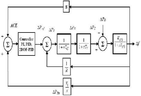
Figure 2 : Single Area ALFC test system with controller
Figure 3: Structure of PID controller
The goal of any controller in a LFC system is that when a disturbance occurs the controller must control the frequency of the system with zero steady state error and less settling time. PI and PID controller used to damp system oscillations, increase stability and reduce steady state error. PID controller continuously calculates an error value as the difference between a desired set point and measured process variable.
Kp, Ki are the gains of proportional, integral part of the controller. These two gains are tuned using PSO.
Kp, Ki, Kd are the gains of proportional, integral, derivative part of the controller. These three gains are tuned using PSO.
( ) (5)
disturbance inputs. The degree of freedom in control system indicates the number of closed loop transfer function that can be adjusted independently. In two degree of freedom controller there is a additional feed forward term which makes a different from the conventional PID controller. Considering that the main advantage of PID controller lies in its simplicity in its structure only the proportional components are added in the feed forward structure.
It consists of Kp,Ki,Kd as in conventional PID and two additional parameters b, c are set points used in the feed forward structure therefore this 2DOFPID is also called as set point weighted PID shown in Fig.4. These set points b and c are assumed as less than one. Due to this feed forward structure of the controller the disturbance due to load change is eliminated and also the controller is robust in case of parameter uncertainties. The load change is given as a step load disturbance. The structure of 2DOFPID is shown in Fig.4
Figure 4: Structure of 2DOFPID controller
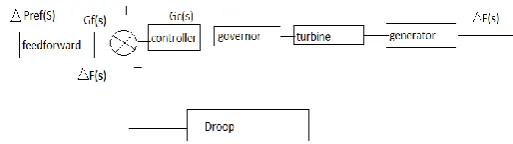
Figure 5: ALFC system with 2DOF-PID controller
The ALFC system with 2DOF-PID controller is shown in Fig 5.The equation Gc(s) and Gf(s) are given by:
Gf(s) = (bKp+cKds2)+(bKpN+Ki)s+Ki(6)
(Kp+KdN)s2+(KpN+Ki)s+KiN
Gc(s) = (Kp+KdN)s2+(KpN+Ki)s+KiN(7)
s(s+N)
III.
OPTIMIZATION USING PARTICLE SWARM
OPTIMIZATION
Particle Swarm Optimization (PSO) is used to explore the search space of a problem to find the parameters required to minimize a particular objective. It is a member of wide category of Swarm Intelligence methods for solving the optimization problems The idea of swarm intelligence based on the observation of swarming habits by animals (such as birds and fish) and the field of evolutionary computation. PSO belongs to the broad class of stochastic optimization algorithms and population-based algorithm that exploits a population of individuals in the search space. The population is called a swarmand the individuals are called particles. Each particle moves with a velocity within the search space, and retains in its memory the best position it ever encountered. In the globalvariant of PSO the best position ever attained by all individuals of the swarm is communicated to all the particles. In the localvariant, each particle is assigned to a neighborhood consisting of a pre specified number of particles. In this case, the best position ever attained by the particles that comprise the neighborhood is communicated among them. Finally, the PSO algorithm maintains the best fitness value achieved among all particles in the swarm, called the global best fitness, and the candidate solution that achieved this fitness, called the global best position.
PSO also keeps the track of the all the best values that the particles have achieved so far. Each particle maintains its position, composed of the candidate solution and its evaluated fitness, and its velocity. It remembers the best fitness value it has achieved, referred to as the individual best position or individual best candidate solution.
The PSO algorithm consists of three steps, which are repeated until some stopping condition is met
1. Evaluate the fitness of each particle
2. Update individual and global best fitness and positions
3. Update velocity and position of each particle
A.Updation of velocity and particle position
velocity. Updating velocity is very important in PSO. The acceleration constants helps in improving the particle position by comparing with the previous particles position and also makes the particle to follow the best neighbour’s direction :
The velocity of each particle in the swarm is
vi(t+1) = w vi (t) + c1 r1 [xˆ i (t) – xi (t)] + c2 r2 [g (t) – xi (t)]
and the position
Xik+1=xik+vik+1 where
Vi(t+1) is the velocity of the particle at t+1th iteration Vi(t) velocity of the particle at t iteration
Xi(k+1) is the position of the particle
c1 and c2 are the acceleration factor constants related to gbest and pbest
r1 and r2 are the random numbers between 0 and 1 i=1,2,3…20
B.PSO parameters Swarm size N=30
Acceleration constants c1=1.5 Acceleration constant c2=1.5
Objective function- ITAE (Integral Time Absolute error) f(x)=ʃ t|e(t)|dt(8)
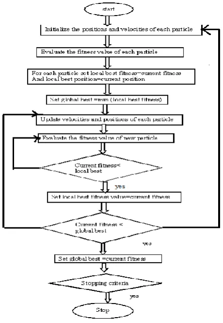
C.Flowchart
The flowchart given below represents the procedure of PSO algorithm implementation.
Figure 6: PSO flow chart
The performance of various control techniques of load frequency control of single area system is analysed in this work through simulation in the MATLAB Simulink environment. The Simulink diagram of ALFC single area test system with 2DOF-PID controller used in this work is shown in Fig.7
Figure 7. Simulink diagram of ALFC single area system
IV.
IV RESULTS AND DISCUSSIONS
A. Case1: analysis of various controllers
undershoot and ITAE. The results are given in table
I.
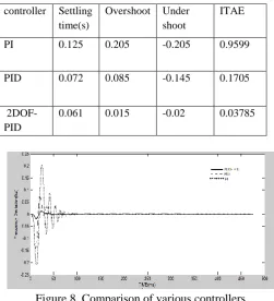
TABLE I. Comparison of various controllers
Figure 8. Comparison of various controllers
From the Fig.8 the proposed controller 2DOF-PID shows less ITAE, less settling time, less overshoot and less undershoot when compared to conventional controllers.
B. case 2: Increase of 10% and 20% Step load disturbance
Increase in Load disturbance of 10% and 20% (1.1pu and 1.2p.u) is given to the ALFC single area test system and its performance is evaluated and results are presented in table II and table III respectively.
TABLE II.10%step load disturbance
Figure 9. 10%step load disturbance
TABLE III.20%step load disturbance
Figure 10. 20% step load Disturbance
Above Fig.9. & Fig.10, show that the 2DOF controller is able to reject disturbance for the increase of 10% and 20% step change in load demand with less ITAE and it exhibits better dynamic performances.
controller Settling
time(s)
Overshoot Under shoot
ITAE
PI 0.125 0.205 -0.205 0.9599
PID 0.072 0.085 -0.145 0.1705
2DOF-PID
0.061 0.015 -0.02 0.03785
controlle r
Settlin g time(s)
Overshoo t
Under shoot
ITAE
PI 0.12 0.2 -0.2 0.9351
PID 0.073 0.082 -0.14 0.1632
2DOF-PID
0.064 0.015 -0.015 0.0364 5
controlle r
Settlin g time(s)
Overshoo t
Under shoot
ITAE
PI 0.13 0.21 -0.215 0.9846
PID 0.079 0.085 -0.145 0.1778
2DOF-PID
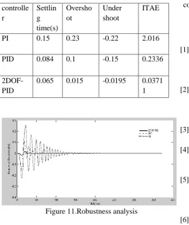
C. case 3: Analysis of 50% Parameter Uncertainty
The change in parameter of the system is considered to check the robustness of the proposed controller. The 2DOF-PID is robust for 50% parameter uncertainty in governor time constant (Tg). The result is presented in table IV
TABLE IV.Robustness analysis
Figure 11.Robustness analysis
Thus the performance of 2DOF-PID seems to be better than conventional controller in terms of dynamic performance like settling time, overshoot, undershoot and performance index (ITAE).
IV.CONCLUSION
By comparing the simulation results of PI, PID, and 2DOF-PID controllers, the performances of the proposed controller proves to be better as it reduces the transient deviations and damp out the frequency for increase in 10% and 20% step load disturbance. Further the proposed controller is robust for ±50% change in governor time constant. It can be extended by changing turbine and generator time constant also. Thus, it is concluded that 2DOF-PID controller in all cases have
lesser settling time, reduced performance index and with less overshoot and undershoot when compared to PI,PID controllers.
V.
Acknowledgment
The authors acknowledge the support provided by the Management, Principal and Faculty of Electrical and Electronics Engineering department of Thiagarajar college of Engineering, Madurai.
VI.
References
[1] D.K.Chaturvedi, P.S.Satsangi , P.K. Kalra “Load frequency control:a generalized neural network approach” Electrical Power and Energy Systems 21(1999)405-415 Elsevier
[2] Dola Gobinda Padhan,Somanath Majhi “ A new control scheme for PID load frequency controller for single area and multi area systems” ISA Transactions 52(2013)242-251 Elsevier
[3] O.I.Elgerd “Electric Energy System Theory;An introduction “Mc Graw Hill.1971
[4] M.K.Sherbiny El “Efficient fuzzy logic load frequency controller”Energy Conversion and Management 43(2002)1853-1863 Elsevier
[5] S.P.Ghosal “Optimizations of PID gains by particle swarm optimizations in fuzzy based automatic generation control”Electric Power Systems research 72(2004)203-212 Elsevier [6] Muwaffaq Irsheid Alomoush “Load frequency
cntrol and automatic generation control using fractional order controllers” Electr Engg(2010)91:357-3688 Springer
[7] Wen tan”tuning of PID load frequency controller for power systems” Energy Conversion and Management 50(2009(1465-1472 Elsevier
[8] V.soni.G.Parmar,M.Kumar and S.Panda “hybrid grey wold optimization-pattern search optimized 2DOF-PID controllers for load frequency control in interconnected thermal power plants”ICTACT journal on soft computing April 2016,volume 06, issue 03.
[9] RV Rao, VJ savsani,DP vakharia “Teaching learning based optimization: an optimization method for continuous non-linear large scale problems”Infinite science 2012;183(10:1-15 controlle r Settlin g time(s) Oversho ot Under shoot ITAE
PI 0.15 0.23 -0.22 2.016
PID 0.084 0.1 -0.15 0.2336
2DOF-PID
[10] P. Kundur.”Power system stability and control”,Tata Mc Graw Hill,2009.
[11] J.Talaq,A.I.Fadel and Basri,”Adaptive Fuzzy Gain Scheduling for Load Frequency control”,IEEE
Transactions on Power
System,Vol.14.No.1,pp.145-150,1999