An approach to a fuzzy problem using the fuzzy Laplace transform under the generalized differentiability

https://doi.org/10.26637/MJM0801/0015

An approach to a fuzzy problem using the fuzzy

Laplace transform under the generalized

differentiability

H ¨ulya G ¨ultekin C

¸ itil

1

*

Abstract

In this paper, the solutions of a second-order fuzzy initial value problem are studied by the fuzzy Laplace transform under the generalized differentiability. An example is solved. Finally, conclusions are given.

Keywords

Second-order fuzzy differential equation, Fuzzy initial value problem, Fuzzy Laplace transform.

AMS Subject Classification 03E72, 34A07, 44A10

1_{Department of Mathematics, Faculty of Arts and Sciences, Giresun University, Giresun, Turkey.} *Corresponding author:1_{[email protected]}

Article History: Received17September2019; Accepted09December2019 c2020 MJM.

Contents

1 Introduction. . . 82

2 Preliminaries. . . 82

3 Main Results. . . 84

4 Conclusion. . . 87

References. . . 87

1. Introduction

There are many approaches to define fuzzy derivative. The first one is Hukuhara derivative[1–3]. But Hukuhara derivative has a drawback. Solution becomes fuzzier as time goes. Thus, fuzzy solution behaves differently from the crips solution. The second one is generalized Hukuhara derivative [4–8]. The third one is Zadeh’s extension principle [9]. Another approach is differential inclusion [10].

Fuzzy Laplace transform is useful to solve fuzzy differen-tial equation. It is found the solution of the fuzzy differendifferen-tial equation satisfying the initial condition by fuzzy Laplace transform directly. Allahviranloo and Barkhordari Ahmadi first introduced fuzzy Laplace transform [11]. In many papers, solution of fuzzy differential equation was studied by fuzzy Laplace transform [12–14].

In this paper, we investigate the solutions of the problem

βu00(t) +δu

0

(t) = [0]α_{, t>0 (1.1)}

u(0) = [Q]α_{, u}0_{(0) = [W]}α_{, (1.2)}

by the fuzzy Laplace transform under the concept of general-ized differentiability, whereβ,δ>0,[0]α= [−1+α,1−α],

Q, and W are symmetric triangular fuzzy numbers with sup-portshq

α,qα

i

,[w_α,wα]and theα−level sets of Q, W are

[Q]α₌h_Q α,Qα

i

=

q+

_q−q

2

α,q−

_q−q

2

α

,

[W]α₌

W_α,Wα

=

w+

w−w

2

α,w−

w−w

2

α

.

This paper is organized as in section 2 Preliminaries, in section 3 Main Results, in section 4 Conclusion.

2. Preliminaries

Definition 2.1. [15] A fuzzy number is a mapping u:R→

[0,1] satisfying the properties{x∈R|u(x)>0}is compact,

u is normal, u is convex fuzzy set, u is upper semi-continuous onR.

LetRFshow the set of all fuzzy numbers.

Definition 2.2. [4] Let be u∈RF. Theα-level set of u is

[u]α_{= [u}

Ifα=0,

[u]0=cl{suppu}=cl{x∈_R|u(x)>0}.

Remark 2.3. [4] The parametric form[u_α,uα] of a fuzzy

number satisfying the following requirements is a validα -level set.

u_αis left-continuous monotonic increasing (nondecreas-ing) bounded on(0,1],

uαis left-continuous monotonic decreasing

(nonincreas-ing) bounded on(0,1],

u_αand uαare right-continuous forα=0,

u_α≤uα,0≤α≤1.

Definition 2.4. [15] Theα−level set of symmetric triangu-lar fuzzy number Q with support[q,q]is

[Q]α=hQ

α,Qα

i

=

q+

_q−q

2

α,q− _q−q

2

α

.

Definition 2.5. [4] Let be u,v∈RF andλ ∈R.u+v and

λu are defined by[u+v]α_{= [}

u]α_{+ [}

v]α

and[λu]α₌

λ[u]α_,

∀α∈[0,1].[u]α_{+ [}

v]α

andλ[u]α

mean the usual addition of two intervals (subsets) ofRand the usual product between a

scalar and a subset of R,respectively.

Definition 2.6. [4,16] Let be u,v∈RF.If u=v+w such that there exists w∈_RF,w is the Hukuhara difference of u and v,it is denoted as w=u v.

Definition 2.7. [4,17] Let be f:[a,b]→_RFand x0∈[a,b].

If there exists f0(x0)∈RFsuch that for all h>0sufficiently small,∃f(x0+h) f(x0), f(x0) f(x0−h)and the limits

hold

lim

h→0

f(x0+h) f(x0)

h =hlim→0

f(x0) f(x0−h)

h =f

0 (x0),

f is Hukuhara differentiable at x0.

Definition 2.8. [4] Let be f:[a,b]→RFand x0∈[a,b].If

there exists f0(x0)∈RF such that for all h>0 sufficiently small,∃f(x0+h) f(x0), f(x0) f(x0−h)and the limits

hold

lim

h→0

f(x0+h) f(x0)

h =hlim→0

f(x0) f(x0−h)

h =f

0 (x0),

f is (1)-differentiable at x0.If there exists f 0

(x0)∈RF such that for all h>0sufficiently small,∃f(x0) f(x0+h),

f(x0−h) f(x0)and the limits hold

lim

h→0

f(x0) f(x0+h) −h =hlim→0

f(x0−h) f(x0)

−h =f

0 (x0),

f is (2)-differentiable.

Theorem 2.9. [7]Let f:[a,b]→_RF be fuzzy function and denote[f(x)]α₌h_f

α(x),fα(x)

i

,for eachα∈[0,1].

(i)If the function f is (1)-differentiable, the lower function

f

α and the upper function fαare differentiable,

h

f0(x)iα=

h

f0

α(x),f 0

α(x)

i

,

(ii)If the function f is (2)-differentiable, the lower function

f

α and the upper function fαare differentiable,

h

f0(x)iα=

h

f

0

α(x),f 0

α(x)

i

.

Theorem 2.10. [7]Let f0:[a,b]→RF be fuzzy function and denote[f(x)]α ₌h_f

α(x),fα(x)

i

, for eachα ∈[0,1],the

function f is (1)-differentiable or (2)-differentiable.

(i)If f and f0 are (1)-differentiable, f0

αand f 0

α are

differ-entiable,hf00(x)iα=hf00

α(x),f 00

α(x)

i

,

(ii)If f is (1)-differentiable and f0 is (2)-differentiable, f0

α

and f

0

α are differentiable,

h

f

00

(x)iα=

f

00

α(x),f 00

α(x)

,

(iii)If f is (2)-differentiable and f0is (1)-differentiable, f0

α

and f

0

α are differentiable,

h

f

00 (x)i

α =

f

00

α(x),f 00

α(x)

,

(iv)If f and f0 are (2)-differentiable, f0

αand f 0

αare

differ-entiable,

h

f00(x)iα=hf00

α(x),f 00

α(x)

i

.

Definition 2.11. [12,13] Let f :[a,b]→RF be fuzzy func-tion. The fuzzy Laplace transform of f is

F(s) = L(f(t)) = ∞ Z

0

e−stf(t)dt

=  lim τ→∞ τ Z 0

e−stf(t)dt,lim

τ→∞ τ

Z

0

e−stf(t)dt



.

F(s,α) =L (f(t))α

=hL

f

α(t)

,L f_α(t)i

,

L

f

α(t)

= ∞ Z

0

e−stf

α(t)dt=τ→lim∞ τ

Z

0

e−stf

α(t)dt,

L f_α(t)

= ∞ Z

0

e−stf_α(t)dt=lim

τ→∞ τ

Z

0

e−stf_α(t)dt.

Theorem 2.12. [12,13]Suppose that f is continuous fuzzy-valued function on[0,∞)and exponential orderαand that f

0

is piecewise continuous fuzzy-valued function on[0,∞).If f is (1)-differentiable,

L

f0(t)=sL(f(t)) f(0),

if f is (2)-differentiable,

Theorem 2.13. [12,13]Suppose that f and f0 are continu-ous fuzzy-valued functions on[0,∞)and exponential orderα

and that f00is piecewise continuous fuzzy-valued function on

[0,∞).

If f and f0are (1)-differentiable,

L

f00(t)=s2L(f(t)) s f(0) f0(0),

if f is (1)-differentiable and f0 is (2)-differentiable,

Lf

00

(t)=−f0(0) −s2

L(f(t))−s f(0),

if f is (2)-differentiable and f0 is (1)-differentiable,

Lf

00

(t)=−s f(0) −s2L(f(t)) f0(0),

if f and f0are (2)-differentiable,

Lf00(t)=s2L(f(t)) s f(0)−f0(0).

Theorem 2.14. [11,13]Let be f(t), g(t)continuous fuzzy-valued functions and c1and c2constants, then

L(c1f(t) +c2g(t)) = (c1L(f(t))) + (c2L(g(t))).

3. Main Results

In this section, we research the solutions of the problem (1.1)-(1.2) by fuzzy Laplace transform under the concept of generalized differentiability. In this paper, (i,j) solution means that u is (i)-differentiable,u0 is (j)-differentiable, i=1,2.

i) (1,1) solution of the problem:

Ifuandu0 are (1)-differentiable, since

L [0]α

= β

s2L(u(t)) su(0) u0(0) +δ(sL(u(t)) u(0)),

we have the equations

L(−1+α) = βs2L(uα(t))−βsuα(0)−βu 0 α(0) +δsL(u_α(t))−δu_α(0),

L(1−α) = βs2L(uα(t))−βsuα(0)−βu 0 α(0) +δsL(uα(t))−δuα(0).

Using the initial values (1.2) , we get

L(u_α(t)) βs2+δs=−1+α

s +βWα+ (βs+δ)Qα,

L(uα(t)) βs2+δs

=1−α

s +βWα+ (βs+δ)Qα.

From this, we obtain

L(u_α(t)) = −1+α

βs3+δs2+ βWα

βs2+δs+

Q

α

s ,

L(uα(t)) =

1−α βs3+δs2

+ βWα

βs2+δs

+Qα

s .

Now, taking the inverse Laplace transform of the above equations, (1,1) solution is obtained as

u_α(t) =

−1+α

δ t

+β

δ

e−βδt−₁

+βWα

δ

1−e−δβt

+Q

α,

uα(t) =

1−α

δ t+

β

δ

e−δβt−₁

+βWα

δ

1−e−δβt

+Q_α,

[u(t)]α_{= [}

u_α(t),uα(t)].

ii) (1,2) solution of the problem:

Ifuis (1)-differentiable andu0 is (2)-differentiable, we have the equations

L [0]α

= β

−u0(0) −s2

L(u(t))−su(0) +δ(sL(u(t)) u(0)),

L(−1+α) = −βu0_α(0) +βs2L(uα(t))−βsuα(0) +δsL(u_α(t))−δu_α(0),

L(1−α) = −βu

0

α(0) +βs

2_L(u

α(t))−βsuα(0) +δsL(uα(t))−δuα(0).

From this, we obtain the equations

βs2L(uα(t))+δsL(uα(t)) =

−1+α

s +βsQα+βWα+δQα

(3.1)

βs2L(u_α(t))+δsL(uα(t)) =

1−α

s +βsQα+βWα+δQα.

(3.2) IfL(uα(t))in the equation (3.1) is replaced by the equation

(3.2), we have

L(u_α(t)) = (1−α)

βs+δ

s2_(β2_s2_−δ2₎

(3.3)

− β δWα

s(β2s2−δ2)

+Qα

s +

β2W_α

β2s2−δ2

Taking inverse Laplace transform of the equation (3.3), the lower solution is obtained as

u_α(t) = (1−α)

  β δ2  

eβδt_+e− δ βt

2 −1

  +1 δ     β

eδβt−_e− δ βt

2δ −t

       

−βWα

δ





eβδt_+e− δ βt

2 −1





+βWα

2δ

eδβt−_e− δ βt

+Q

α.

Similarly, the upper solution is obtained as

uα(t) = (−1+α)

  β δ2  

eδβt_+e− δ βt

2 −1

  +1 δ     β

eδβt−_e− δ βt

2δ −t

       

−βWα

δ





eβδt+_e− δ βt

2 −1





+βWα

2δ

eδβt−_e− δ βt

+Q_α.

iii) (2,1) solution of the problem:

Ifuis (2)-differentiable andu0 is (1)-differentiable, since

L [0]α

= β

−su(0) −s2

L(u(t)) u0(0) +δ(−u(0) (−sL(u(t)))),

we have the equations

L(−1+α) = −βsuα(0) +βs2L(uα(t))−βu 0 α(0)

−δuα(0) +δsL(uα(t)),

L(1−α) = −βsu_α(0) +βs2L(u_α(t))−βu0_α(0)

−δu_α(0) +δsL(u_α(t)).

That is,

L(u_α(t)) = 1−α

βs3+δs2+ βWα

βs2+δs+

(βs+δ)Q

α

βs2+δs ,

L(uα(t)) =

−1+α βs3+δs2+

βW_α

βs2+δs+

(βs+δ)Q_α

βs2+δs .

From this, (2,1) solution is obtained as

u_α(t) =

₁₋

α

δ t+

β

δ

e−δβt−₁

+βWα

δ

1−e−βδt

+Q

α,

uα(t) =

₋₁₊

α

δ t+

β

δ

e−βδt−₁

+βWα

δ

1−e−δβt

+Q_α,

[u(t)]α_{= [u}

α(t),uα(t)]. iv) (2,2) solution of the problem:

Ifuandu0are (2)-differentiable, since

L [0]α

= β

s2L(u(t)) su(0)−u0(0) +δ(−u(0) (−sL(u(t)))),

the equations

L(−1+α) = βs2L(u_α(t))−βsu_α(0)−βu0_α(0)

−δuα(0) +δsL(uα(t)),

L(1−α) = βs2L(uα(t))−βsuα(0)−βu 0 α(0)

−δu_α(0) +δsL(u_α(t))

are obtained. These yield

βs2L(u_α(t))+δsL(uα(t)) =

−1+α

s +βsQα+βWα+δQα,

(3.4)

βs2L(uα(t))+δsL(uα(t)) =

1−α

s +βsQα+βWα+δQα.

(3.5) IfL(uα(t))in the equation (3.5) is replaced by the equation

(3.4), we have

L(u_α(t)) = (−1+α)

βs+δ

s2_(β2_s2_−δ2₎

(3.6)

− β δWα

s(β2s2_−δ2₎+

Q

α

s +

β2Wα

β2s2_−δ2.

Taking inverse Laplace transform of the equation (3.6), the lower solution is obtained as

u_α(t) = (−1+α)

  β δ2  

eδβt_+e− δ βt

2 −1

  +1 δ     β

eδβt−_e− δ βt

2δ −t

       

−βWα

δ





e

δ βt_+e−

δ βt

2 −1





+βWα

2δ

eδβt−_e− δ βt

+Q

Similarly, the upper solution is obtained as

uα(t) = (1−α)





β

δ2





eβδt_+e− δ βt

2 −1





+1

δ



  

β

eδβt−_e− δ βt

2δ −t



  



  

−βWα

δ





eβδt_+e− δ βt

2 −1





+βWα

2δ

eδβt−_e− δ βt

+Q_α.

Example 3.1. Consider the solutions of the problem

u00(t) +u0(t) = [0]α_,

t>0,

u(0) = [0]α_{, u}0_{(0) = [1]}α

by fuzzy Laplace transform, where

[0]α_{= [−}

1+α,1−α],[1]α_{= [}

α,2−α].

(1,1) solution is

u_α(t) = (−1+α) t+e−t+α 1−e−t

= α(t+1)−t−e−t,

uα(t) = (1−α) t+e −t

+ (2−α) 1−e−t

= t+2−e−t−α(t+1),

[u(t)]α_{= [u}

α(t),uα(t)].

(1,2) solution is

u_α(t) = (1−α) et−t−2−(2−α)

et+e−t

2 −1

+α

et−e−t

2

= α(t+1)−t−e−t,

uα(t) = (−1+α) et−t−2

−α

_et_+e−t

2 −1

+ (2−α)

_et_−e−t

2

= t+2−e−t−α(t+1),

[u(t)]α_{= [u}

α(t),uα(t)].

If

∂uα(t)

∂ α ≥ 0,

∂uα(t)

∂ α ≤0,uα(t)≤uα(t),

u0_α(t) ≤ u0_α(t),u

00

α(t)≤u 00

α(t),

(1,1) solution is a valid fuzzy function. If

∂u_α(t)

∂ α ≥ 0,

∂uα(t)

∂ α ≤0, uα(t)≤uα(t),

u0_α(t) ≤ u0_α(t), u

00

α(t)≤u 00

α(t),

(1,2) solution is a valid fuzzy function. For (1,1) solution, since

∂uα(t)

∂ α =t+1>0,

∂uα(t)

∂ α =−t−1<0,

uα(t)−uα(t) =2(1−α) (t+1)≥0,

u0_α(t)−u0_α(t) =2(1−α)≥0,u

00

α(t)−u 00

α(t) =0,

(1,1) solution is a valid fuzzy function. Similarly, (1,2) solution is a valid fuzzy function. Also, for (1,1) and (1,2) solutions, since

u₁(t) =1−e−t=u1(t),

u₁(t)−u_α(t) = (1−α) (t+1) =uα(t)−u1(t),

(1,1) and (1,2) solutions are symmetric triangular fuzzy num-bers for any t>0time. (2,1) solution is

u_α(t) = (1−α) t+e−t−2+ (2−α) 1−e−t

= t−e−t+α(1−t),

uα(t) = (−1+α) t+e −t₋₂

+α 1−e−t

= 2−t−e−t+α(t−1),

[u(t)]α_{= [u}

α(t),uα(t)].

(2,2) solution is

u_α(t) = (−1+α) et−t−α

_et_+e−t

2 −1

+ (2−α)

_et_−e−t

2

= t−e−t+α(1−t),

uα(t) = (1−α) et−t

−(2−α)

et+e−t

2 −1

+α

et−e−t

2

= 2−t−e−t+α(t−1), [u(t)]α_{= [}

u_α(t),uα(t)].

If

∂uα(t)

∂ α ≥ 0,

∂uα(t)

∂ α ≤0, uα(t)≤uα(t),

u0_α(t) ≤ u0_α(t), u

00

α(t)≤u 00

(2,1) solution is a valid fuzzy function. If

∂u_α(t)

∂ α ≥ 0,

∂uα(t)

∂ α ≤0,uα(t)≤uα(t),

u0_α(t) ≤ u0_α(t),u

00

α(t)≤u 00

α(t),

(2,2) solution is a valid fuzzy function. For (2,1) solution, since

∂uα(t)

∂ α =1−t,

∂uα(t)

∂ α =t−1,

uα(t)−uα(t) =2(1−α)(1−t),

if t≤1,we have∂uα(t) ∂ α ≥0,

∂uα(t)

∂ α ≤0,uα(t)≤uα(t).Also,

since

u0_α(t)−u0_α(t) =2(1−α)≥0, u

00

α(t)−u 00

α(t) =0,

(2,1) solution is a valid fuzzy function for t ≤1.Similarly, (2,2) solution is a valid fuzzy function for t≤1. In addition, for (2,1) and (2,2) solutions, since

u₁(t) =1−e−t=u1(t),

u₁(t)−u_α(t) = (α−1) (t−1) =uα(t)−u1(t),

(2,1) and (2,2) solutions are symmetric triangular fuzzy num-ber for any t>0time.

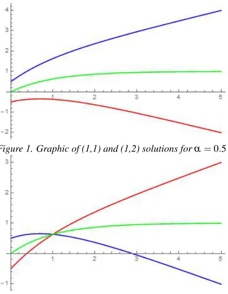
Figure 1. Graphic of (1,1) and (1,2) solutions forα=0.5

Figure 2. Graphic of (2,1) and (2,2) solutions forα=0.5

Blue→y_α(t)

Red→y

α(t)

Green→y₁(t) =y

1(t)

4. Conclusion

In this paper, we study the solutions of a second-order fuzzy initial value problem using the fuzzy Laplace transform under the generalized differentiability. We use symmetric triangular fuzzy number, Hukuhara difference, the properties of fuzzy Laplace transform and fuzzy arithmetic. We solve an example related to the problem. We obtain that (1,1) and (1,2) solutions are valid fuzzy functions and (2,1) and (2,2) solu-tions are valid fuzzy funcsolu-tions fort≤1.Also, we obtain that all of the solutions are symmetric triangular fuzzy numbers for anyt>0 time.

References

[1] _{J. J. Buckley, T. Feuring, Fuzzy differential equations,}

Fuzzy Sets and Systems, 110(1)(2000), 43–54.

[2] _{O. Kaleva, Fuzzy differential equations,Fuzzy Sets and}

Systems, 24(3) (1987), 301–317.

[3] _{H. G¨ultekin, N. Altınıs¸ık, On solution of two-point fuzzy}

boundary value problems, The Bulletin of Society for Mathematical Services and Standards, 11(2014), 31–39.

[4] _{A. Khastan, J. J. Nieto, A boundary value problem for}

second order fuzzy differential equations,Nonlinear Anal-ysis, 72(9-10) (2010), 3583–3593.

[5] _{B. Bede, S. G. Gal, Generalizations of the}

differentiabil-ity of fuzzy-number-valued functions with applications to fuzzy differential equations,Fuzzy Sets and Systems, 151(3)(2005), 581–599.

[6] _{B. Bede, I. J. Rudas, A. L. Bencsik, First order linear}

fuzzy differential equations under generalized differentia-bility,Information Sciences, 177(7)(2007), 1648–1662.

[7] _{A. Khastan, F. Bahrami, K. Ivaz, New results on multiple}

solutions for nth-order fuzzy differential equations under generalized differentiability,Boundary Value Problems, (2009), 1–13.

[8] _{H. G¨ultekin C¸ itil, The relationship between the solutions}

according to the noniterative method and the generalized differentiability of the fuzzy boundary value problem,

Malaya Journal of Matematik, 6(4) (2018), 781–787.

[9] _{M. Oberguggenberger, S. Pittschmann, Differential}

equa-tions with fuzzy parameters,Mathematical and Computer Modelling of Dynamical Systems, 5(3)(1999), 181–202.

[10] _{E. H¨ullermeier, An approach to modelling and simulation}

of uncertain dynamical systems,International Journal of Uncertainty, Fuzziness and Knowledge-Based Systems, 5(2)(1997), 117–137.

[11] _{T. Allahviranloo, M. Barkhordari Ahmadi, Fuzzy Laplace}

transforms,Soft Computing, 14(3)(2010), 235–243.

[12] _{S. Salahshour, T. Allahviranloo, Applications of fuzzy}

Laplace transforms,Soft Computing, 17(1)(2013), 145– 158.

[13] _{K. R. Patel, N. B. Desai, Solution of variable coefficient}

fuzzy differential equations by fuzzy Laplace transform,

[14] _{K. R. Patel, N. B. Desai, Solution of fuzzy initial value}

problems by fuzzy Laplace transform,Kalpa Publica-tions in Computing, 2(2017), 25–37.

[15] _{H.-K. Liu, Comparison results of two-point fuzzy}

bound-ary value problems,International Journal of Computa-tional and Mathematical Sciences, 5(1)(2011), 1–7.

[16] _{M. L. Puri, D. A. Ralescu, Differentials of fuzzy}

func-tions,Journal of Mathematical Analysis and Applications, 91(2)(1983), 552–558.

[17] _{B. Bede, Note on “Numerical solutions of fuzzy}

differen-tial equations by predictor-corrector method”, Informa-tion Sciences, 178(7)(2008), 1917–1922.

? ? ? ? ? ? ? ? ?

ISSN(P):2319−3786 Malaya Journal of Matematik

ISSN(O):2321−5666