Abstract- The indentation of layered viscoelastic solids is a
nonlinear and time-dependent problem. Consideration of the time-dependency of viscoelasticity and inclusion of the friction complicates the analysis of the problem. This paper presents a numerical study to detect the indentation response of a viscoelastic solid layered by an elastic layer and indented by a flat rigid indenter. Interfacial indentation stresses and deformations at the indentation surface are completely determined. Furthermore, effects of two layer characteristics, layer thickness and layer stiffness, and two interfacial frictional parameters, micro-slip and coefficient of friction, upon the indentation response are investigated.
Index Term— finite element method (FEM), friction,
indentation problem, viscoelasticity.
I. INTRODUCTION
Interfacial indentation stresses and deformations at the indentation surface investigate the response of the intended viscoelastic solids. The indentation response depends on the geometry of the system, material properties of the indented solids and frictional parameters at the indentation surface. Under the action of normal loads, indentation press ure and tangential stresses are built up at the indentation surface. Such stresses are compensated by the indentation depth and the relative tangential displacements, respectively. The indentation response may be controlled by layering the indented solid. In addition to the layer characteristics, the indentation response is affected by the interfacial frictional parameters at the indentation surface. Such type of problems is belonging to a nonlinear and time-dependent class of contact problems. The nonlinearity is due to the continuous changing of the boundary conditions throughout the indentation surface. On the other hand, the time dependency is due to the time dependent stress -strain relationships for either creep or stress relaxation responses of viscoelatic materials.
Analytical solutions for the indentation of linear isotropic viscoelastic solids have been obtained by using the
A. G. El-Shafei, Associate professor, Department of Mechanical Design and Production Engineering, College of Engineering, Zagazig University,
Zagazig, 44511, Egypt, e-mail: [email protected]. Currently, on sabbatical leave to College of Engineering, Jazan University,
Jazan 45142, Kingdom of Saudi Arabia
correspondence principle of viscoelasticity [1]. The elastic modulus is replaced by the hereditary integral of the relaxation modulus to obtain an expression for the pressure distribution for a spherical indentation of a linear viscoelastic body [2]. This model provided a negative pressure with the reduction of the contact area [3]. This drawback is overcome by the formulation [4]. For incompressible and compressible viscoelastic materials, the contact radius and the contact pressure for frictionless indentation of a viscoelastic layer bonded to a rigid substrate are obtained by [5]. The Maxwell model is used to obtain an expression for the indentation depth for simple load histories [6]. Utilizing the Prony series, the creep response is detected from the slope of the measured indentation depth [7]. The solution for the indentation of viscoelastic material by of an axisymmetric flat punch [8] is extended for the indentation of a viscoelastic half space by a spherical tip indenter [9]. Reference [10] derived constitutive equations governing the time-dependent indentation of an axisymmetric indenter into a fractional viscoelastic h alf-space. In spite of the limitations of these analytical models for simple geometry and loading conditions, they gave an insight into the indentation of viscoelastic solids. However, validation of the indentation theory of viscoelastic solids needs to be carefully assessed by the comparison with experimental tests or accurate numerical solutions.
Numerical solutions for the indentation problems of viscoelastic or layered solids are obtained by using the FEM. The indentation of a viscoelastic layer by a rigid spherical indenter is analyzed in [11]. A comparison for some instants of time is made with the analytical solution [2]. The frictionless indentation problem of a compressible viscoelastic layer bonded to a rigid substrate is modeled using the FEM [12]. Results of this model are compared with the solutions that obtained by the correspondence principle of viscoelasticity [5]. Based on the asymptotic solutions [13], a load–depth curve is obtained for an arbitrary ratio of indenter radius to layer thickness for the indentation of a flat punch into a compressible elastic layer bonded to a rigid substrate [14]. Indentation tests of glassy polymeric materials to analyze the behavior of materials at micron and submicron indentations are investigated in [15]. Nano-indentation processes, to study
Interfacial Indentation Stresses and
Deformations of Elastically Layered
Viscoelastic Solids
loading and unloading stress and strain fields of both bulk materials and thin films, are investigated using the FEM [16].
The objective of this paper is to determine the quasistatic frictional nonlinear time-dependent indentation response; indentation pressure, indentation depth, tangential stress and relative tangential displacement, for a viscoelastic solid layered by elastic layer and indented by a flat rigid indenter. Furthermore, effects of the layer characteristics and interfacial frictional parameters upon the indentation response are investigated. The problem will be handled numerically using a 2D FE model. The constitutive equations of viscoelasticity presented by the Schapery model [17] are transformed into a recursive incremental form suitable for the FE formulations. The variational inequality constrained model of the indentation problem is solved by the incremental convex programming method [18], while the Lagrange multiplier method is used to enforce the inequality contact constraints. The local-nonlinear friction law [19] is adapted to model friction at the indentation surface.
II. STATEM ENTOFTHEINDENTATIONPROBLEM
Consider the indentation problem of a viscoelastic substrate layered by an elastic layer and indented by a rigid indenter, shown in Fig. 1. Assuming that the system occupies a domain
Ω in RN, N ≤ 3. On the portions of boundary Γd and Γf, displacement and normal traction are prescribed, respectively.
Γc is the portion of the boundary that contains material surfaces which candidate to come into contact upon the application of loads. In addition to the boundary conditions that prescribed on the boundary Γd, a set of contact conditions must be imposed throughout the indentation surface Γc.
Fig. 1. A representation of the indentation problem
This indentation problem is belonging to a class of nonlinear initial boundary value problems having inequality constraints at the indentation surface. If the applied loads vary slowly with time, the inertia term may be neglected. This leads to a quasistatic problem defined by the following equilibrium equations with the associated boundary conditions:
) , ( 0 )
( ,j fi inΩ t ij u
(1)
) , ( )
(
) ( 0
t Γ on n
F
Γ on u
f j
ij i
d i
u
(2)
where ζij(u) is the Cauchy stress tensor which is a function of the displacement vector u, fi is the body force per unit volume, ui is the prescribed displacement, n is the outward normal vector to Γf, Fi is the prescribed normal traction per unit area and t is the time. The elastic material is assumed to obey Hooke’s law, while the constitutive relationships for linear homogeneous non-aging viscoelastic materials can be expressed by [17], such that
) , ( ) , ( ) ( )
, (
0
t Ω in t d t
t x e t t C
t kl k
t
ijkl
ij
x (3)
where xis the space variable and Cijklis the fourth order tensor of relaxation modulus that relating the second order Cauchy stress tensor ζij to the second order infinitesimal strain tensor
ekl.
Instead of using the classical Coulomb's law of friction, a local-nonlinear friction law is adopted to model friction at the indentation surface. According to the welding shearing and ploughing theory [20], the indentation surface may be composed of micro-slip and macro-slip contact zones. Micro-slip contact zones involve relative micro-Micro-slip displacements occur by tangential stresses below the friction capacity. This frictional capacity depends on the indentation pressure, the coefficient of friction and the tangential contact stiffness. On the other hand, macro-slip contact zones exhibit relative macro-slip displacements occur when the relative tangential displacement reaches a certain limit that depends on the tangential stiffness at the indentation surface. The nonlinear relationship between the tangential stress vector σT and the relative tangential displacement vector uT can be expressed as [19]
T T T n
T
u u u u σ u
σ ( ) ( )( )
(4)
where σn(u) is the indentation pressure vector, μ is the static coefficient of friction and is a continuous, monotone and
real-valued function of the relative tangential displacement, which defined by the following form:
mode c macroscopi for
1
mode c microscopi for
T T T
T
if if
u u u
u
(5)
where the micro-slip parameter ε is a positive parameter that used as a measure to the tangential contact stiffness. It is noticed that the macro-slip displacement occurs only when the relative tangential displacement uT is greater than the value of ε. An interesting feature of the local-nonlinear friction law is that the response depends on two frictional parameters, the coefficient of friction and the micro-slip parameter.
In addition to the boundary conditions (2) and based on the local-nonlinear friction model, the following contact conditions must be imposed for all contact points at the indentation surface:
ΓF
Rigid indenter
Viscoelastic substrate
Elastic layer
F
Γd
n T
) , ( )
( ) ( )
(
0 ) ( , 0 ) ( , 0
t Γ on c
T T T n
T
n n n
n n n
u u u u σ u
σ
G u σ u g
u G
(6)
where Gn is the normal gap function. For the ith contact pair on the indentation surface Γc, uniui.ni is the component of the unilateral normal displacement un, ni is the outward normal vector to Γc, gni is the current gap measured along the outward normal. Equation (6) describes boundary conditions at the indentation interface, such that, the first inequality represents the compatibility contact constraints, the second inequality states that no tens ile normal stresses can develop, while the third condition implies that the indentation pressure can only be nonzero when there is contact. The last equation expresses the induced tangential stress due to friction according to the adopted local-nonlinear friction model, defined by (4).
III. THEVARIATIONALFORM ULATIONOFTHEPROBLEM
The principle of virtual work is an equivalent formulation of equilibrium and is called the weak form of equilibrium. Since no constitutive equations enter a priori the weak form, it is valid for all problem classes. The weak form of the equilibrium equation (1) can be written as
f c
Γ Γ
T T T T
Ω T Ω
T
dΓ dΓ
dΓ
dΩ 0
)
(u u f u F u λ
σ
e
(7)
where e is the infinitesimal strain vector corresponding to the virtual displacement vector δu and λT is the tangential force vector at the indentation surface. The first three integrals of (7) represent the virtual work due to internal stresses, body force and surface traction, respectively. The last integral is the virtual work due to the tangential force. Since the tangential force depends on the normal indentation force and the relative tangential displacement, as stated by (4), this force is considered to be a dependent variable. Consequently, such a force can be treated as an applied force working on the virtual tangential displacement δuT.
According to [21] and the extension to consider friction [22], define V to be a space of an admissible displacement, and v is a displacement vector, virtual displacement, belonging to V, such that v = 0 on Γd and a subset K of V consisting of all admissible displacement v in V for which un –
gn ≤ 0 at all points on the indentation surface Γc. Let u be the solution of the problem, the inequality constrained variational model for frictional indentation can be expressed as ;
Find the admissible displacement vector u in set K such that )
( ) , ( ) , ( ) ,
(uvu J uv J uu F vu
a (8)
for all admissible displacements v in K
) , (uv
a is the virtual work by the internal stress ζij(u) and strain eijcaused by the virtual displacement v, such that
Ω
dΩ a(u,v u) ij(u)
e
ij(v u)(9)
Jε(u, v) is the virtual work by the tangential contact forces on the virtual displacements v, such that
c Γ
T
n dΓ
J(u,v) λ (u) (u )
(10)
where φε is the primitive of ,(uT)(uT), defined as
T T
T T
T
if if
u u
u u
u
2 / 2 / 2
(11)
F(v - u) is the virtual work done by both body force and surface traction, respectively, on the virtual displacement v, such that
f
Γ Ω
dΓ dΩ
F(v u) f.v F .v
(12)
The inequality constrained model (8) is a statemen t of the virtual work principle for deformable bodies. The actual indentation surface depends on the solution u, which is not known in advance. The inequalities (6) constrain the displacement field u, and consequently, lead to variational inequalities cons traints. Such variational inequalities can't be directly applied to solve the indentation problem. The Lagrange multiplier method is adopted to incorporate such inequality constraints into the model. Accordingly, the variational inequality constrained model (8) could be transformed into unconstrained model by relaxing the inequality constraints (6). This is done by directly adding (6) to (7), such that
0 ) ( )
(
c c
f
Γ
n n Γ
T T T
Γ T Ω
T Ω
T
dΓ dΓ
dΓ dΓ
dΩ
G λ λ
u
F u f
u u
σ e
(13)
where λn is the Lagrange multiplier vector, which physically equivalents to the normal indentation force vector. The last term of (13) is known as the Lagrangian function. Since both
δu and δλn are varied independently, variation of (13) leads to the following set of equations:
0 )
(
c c
f
Γ n n Γ
T T T
Γ T Ω
T Ω
T
dΓ dΓ
dΓ dΓ
dΩ
G λ λ
u
F u f
u u
σ e
(14-a)
0
c Γ
n nG dΓ
λ
(14-b)
which represent the variational inequality form of the equilibrium equations for the frictional indentation problem with a local-nonlinear friction law. The last integral of (14-a) is the virtual work of the Lagrange multiplier along the variation of the normal gap function Gn, while (14-b) describes the enforcement of the inequality contact constraints (6).
IV. THEFINITEELEM ENTMODELOFTHEPROBLEM
convex programming method [18] with the Lagrange multiplier method is applied to transform the variational inequality constrained model (8) into a sequence of unconstrained models of the form defined by (14). Each one of these unconstrained models is manipulated at one increment of load. Solution of the incremental equilibrium eq uations yields the incremental indentation response. The progression from one model to another depends on the predicted contact events in that model, such that each model has only one additional contact constraint more than the preceding one. Therefore, th e transformation of the original constrained model occurs in an incremental adaptive procedure, such that the total number of increments or unconstrained models does not exceed the number of contact events that detected along the loading history. This adaptive procedure is applied to problems having neither geometrical nor material nonlinearity, and consequently, no iterative scheme is required. Such adaptive procedure is successfully used to predict the time-dependent response of viscoelastic and thermoviscoelastic frictional contact problems [23] and [24], respectively. Following is the formulation of the nonlinear time-dependent frictional contact model.
A. Visccoelastic Constitutive Equations
The first point is concerned with the recasting of the constitutive equations of viscoelasticity into a recursive incremental form suitable for the FE implementation. Generally, working on the constitutive equations (3) leads to the requirement of solving a set of integrals [25]. To overcome this difficulty the constitutive equations will be transformed into a recursive incremental form. Once the time domain is divided into discrete intervals Δt, such that tn+1 = tn+Δt, and knowing the stress state
ij(x,tn) at the time tn, the stress state at time tn+1 can be expressed as) , ( ) , ( ) ( )
,
( 1
0 1
1
t Ω in t d t
t e t t C
t kl
n t
ijkl n
ij
n
x x
(15)
The stress increment from time tn to time tn+1 is given by
t d t
t e C
t d t
t e t t C
t t
t
kl t
ijkl t
t
kl n
ijkl
n R ij n
ij n
ij
n n
n
) , ( Δ
) , ( ) (
) , ( Δ ) , ( Δ ) , ( Δ
0 1
1 1
1
1
x x x x
x
(16)
According to the Wiechert model [26], the fourth order relaxation modulus tensor Cijkl, for homogeneous and non-aging viscoelastic materials, can be expressed as
mijkl n t t M
m m ijkl ijkl
n
ijklt t C C
C ( )/
1 1
1
exp
(17)
where
m ijkl m ijkl m
ijkl
C
(no sum on i, j, k , l) (18)where Cijkl is the equilibrium spring constant, m ijkl C , m
ijkl
and
m ijkl
are the spring constant, dashpot coefficient and relaxation time, respectively, of the mth Maxwell element, and M is the number of Maxwell elements that used to model the mechanical response of the material. Assuming that the rate of change of the strain within the time step is constant, the incremental strain rate can be expressed ast e e t
t
e kl
kl kl
(x, )
(19)
Substituting of (17) and (19) into (16) and then evaluating the integrals, yields
M
m
n m ij t
kl ijkl kl ijkl n
ij t C e C e S t
m ijkl
1 /
1) (exp 1) ( )
, (
Δ x (20)
where
) exp 1 (
1 /
1
m ijkl t M
m m ijkl ijkl
ijkl
t C
C
(21)
exp / ( )(1 exp / )m ijkl m
ijkl t
n kl m ijkl t
n m ij n m
ij t S t t e t
S (22)
B. Modeling of the Indentation Surface
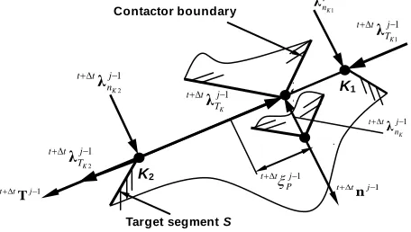
The second point is the modeling of the indentation surface considering friction. The indentation interface is modeled by the node-to-segment contact approach [27], where the contactor nodes are coming into contact with the target segments. In the context of the FEM, both contactor and target are discretized into quadrilateral four node finite elements. The non-penetration condition, defined by the first inequality of (6), is tested for all contactor contact nodes. A typical contact set composed of a contactor physical contact point P
touching a target segment S, after (j-1) increments at the time
t+Δt, and the corresponding indentation forces are shown in Fig. 2.
The physical contact point P initially penetrated the target segment S along the normal vector n taking the position K. Elimination of this penetration locates the point K in the position P. Position of the point P is a function of the natural coordinate ξP measured from the center of the target segment. This position can be expressed in terms of the positions of points K1 and K2 of the target segment S. The target segment
1) K
Fig. 2. Modeling of the indentation surface.
1
t j t
T
Contactor boundary
1
j
P t
t
1
t j t
n 2) P
Target segment S
1
j
n t t
K
λ
1 1
j
T t t
K λ
1
j
T t t
K λ
1 2
j
T t t
K λ
K1
K2
1 2
j
n t t
K λ
1
1
j
n t t
that contains the point P is detected by the dot product of the tangent vector T and the vector of projection of the node K on the normal direction, such that
( )
0)
( 1 1 1
1 1
j P t t j P t t j K t t j P t t j P t t x x x (23)
where j1 K t t
x and j1 P t t
x are the position vectors of the node
K and the physical contact point P, respectively. Since j1 P t t
x
is a function of j1 P t
t
, solution of (23) yields the value of 1 j P t t
.For the shown contact set, the normal indentation depth
1 j n
u
, the normal indentation force vector j1
n
λ
, the
relative tangential displacements j1
T
u
and the tangential
force vector j1
T
λ
can be expressed, respectively, as
) ( 1 1 1 1 1 1 1 1 1 1 1 1 1 j c t t j T t t j T t t j T t t j t t j T t t j T t t j n t t j n t t j n t t j t t j n t t j n t t Γ on u u T T C λ u C C λ u C (24)
where ttuj1is the displacement vector, and C
n and CT are operator vectors that working on the contact constraints, and defined by 1 2 1 1 2 1 1 1 1 2 1 1 2 1 1 1 ) 1 ( ) 1 ( ) 1 ( ) 1 ( j t t p t t j t t p t t j t t j T t t j t t p t t j t t p t t j t t j n t t T T T C n n n C (25)
According to the local-nonlinear friction model, the tangential force vector in a contact point belonging to the micro -slip zone can be expressed as
1 1 1 1 1 j T t t j T t t j T t t j n t t j T t t u u u λ λ (26)
In the micro-slip contact zones, the tangential contact force should be compensated by a tangential contact stiffness, which should be incorporated into the equilibrium equations of the contact system. Differentiation of (26) with respect to the relative tangential displacement vector yields the following definition of the tangential contact stiffness, in the micro -slip contact zones, such that
1 1 1 1 j n t t j T t t j T t t j T t t d d K λ u λ (27)
Based on the spatial dis cretization of the geometry at the indentation surface, the tangential stiffness KT for the shown contact set can be expressed as
T j T t t j T t t j T t t j T t t
K 1 1
1
1
C C
K (28)
Considering (25), (26) and (28), and for all contact constraints,
1 j c t t Γ
i , let us define the following vectors and matrix:
} { } { } { } { } { } { } { } { 1 1 1 1 1 1 1 1 1 1 1 1 1 1 1 1 1 1 1 j n t t j n t t j n t t j t t j n t t j n t t j i t t j n t t j n t t j n t t j n t t j n t t j n t t j n t t j n t t j n t t j n t t j n t t j n t t j T t t j T t t j T t t j T t t i i T i i i i i i i i i i g λ λ λ C C g u C u C G λ C C λ λ C λ λ C λ λ (29-a) 1 1 1 1 1 & , ] [
j
c t t j mic t t j mic t t j T t t j T t
t Γ Γ Γ
m m
K
K (29-b)
These vectors and matrix define the terms at the end of (j-1) increment; j1
n t t
g is the violation vector of the normal gaps,
1 j n t
t λ and j1 T t
t λ are the accumulated normal indentation and tangential force vectors, respectively, and j1
T t t
K is the tangential stiffness matrix for all contact points belonging to
micro-slip contact zones j1 mic t
t Γ . The vector n t
tλ is the incremental Lagrange multiplier vector which physically represents the incremental normal indentation force vector.
C. Incremental Form of the Equilibrium Equations
The last point is the incremental form of the variational inequality model. Assuming that the response is completely known at time t and (j-1) increments have been performed to obtain the solution at time t+Δt. Also, through the time step Δt, j1
c
t is the elapsed or consumed time and trj is the
remaining time, such that j
r j
c t
t t
1 . To obtain the
solution for the jth increment of time t+Δt, the variational inequality form of the equilibrium equations, defined by (14), are reformulated into a discrete and incremental form utilizing the FEM.
Based on the residual increment of time j1
r
t , the relaxation modulus matrix Cof the viscoelastic material, previously defined by (21), can be expressed as
M m t m j r j tt ijklm
j r t 1 / 1 1 ) exp 1 (
1 1
η C
C
(30)
Substituting of (20) into the first integral of (14-a) yields
Ω j R t t T j t t Ω j t t T j t t Ω j t t j t t T j t t Ω T dΩ dΩ dΩ dΩ T T T 1 1 1 ) ( σ B u σ B u u B C B u u σ e
(31)and the third integrals, respectively, of (14-a) can be expressed as
f
T T
f
Γ
t t j t t Ω
t t j t t Γ
T Ω
T
dΓ dΓ dΓ
dΓ
F u
f u F
u f
u
(32)
The fourth integral of (14-a) can be expressed by substituting the first of (29-a) and (29-b) into the fourth integral of (14-a) and then linearization, this yields
dΓ
dΓ Tj t t j
t t Γ
j T t t j t t Γ
T T t
c
T
c
)
( λ 1 K 1 u
u λ
u
(33)
Note that the second term of the last equation is only applied to micro-slip contact zones j1
mic t
t Γ . Also, the last integral of
(14-a) can be expressed by substituting the second and third Eqs. of (29-a) into the last integral of (14-a), and then linearization, this yields
c T
c Γ
j n t t j n t t j n t t j t t Γ
n
n dΓ ( )dΓ
1
1 λ
C λ
u G
λ
(34)
The enforcement of the contact constrains are manipulated by (14-b). Substituting the third and fourth Eqs. of (29-a) into (14-b), and then linearization, yields
c
T T
c Γ
j n t t j t t j n t t j n t t Γ
n
n dΓ [( ) ]dΓ
1 1
g u
C λ
G
λ
(35)
With the theory of variation, (31) to (35) can be arranged in the following matrix form:
1
1 1 1 int 1
1 1
1
] 0 [
j n
j T j n j t
t
j n j t t j
n
j n j T j t t
T
g
λ λ F F f
λ u
C
C K
K
(36)
Kj-1 is the overall stiffness matrix defined by the first integral of the R.H.S. of (31). 1
int
j
F is the contribution of the internal force vector due to both the internal stresses and material damping. This contribution is defined by the second and third integrals of the R.H.S. of (31).
As mentioned previously, the space domain of the problem is discretized into finite elements. Element equations are evaluated by using Gauss quadrature integration scheme [28]. The solution procedure for each increment involves three main modules. The first one is the solution of the equilibrium equations (36), considering all active contact constraints, to obtain the incremental displacement and normal indentation force vectors. The second module is concerned with the detection of the incremental scale factor based on the detected contact event and updating active and inactive contact constraints. This is done according the developed adaptive incremental procedure. Based on the calculated scale factor, the last module is devoted to update the incremental and accumulated vectors of internal stresses and the whole indentation response.
D. Verification of the Model
In the literatures concerning viscoelastic stress analysis problems, results are verified by the comparison with the analytical solutions based on either the Laplace transformation or the elastic-viscoelastic correspondence principle [29]. In these analytical models, the contact body is modeled as a half-space, which is misleading when real problems are considered. Therefore, comparison of results with the elastic-viscoelastic correspondence principle-based solutions is not valid. Reference [12] adopted a comparison scheme, in which only the instantaneous viscoelastic contact pressure is compared with the corresponding equivalent elastic solution.
Validation of the present model is focused on three distinct areas; the use of the Wiechert model to simulate the linear response of viscoelastic material, the contact algorithm to solve viscoelastic contact problems and the use of the local-nonlinear friction law to model friction at the indentation surface. The first two points are completely presented in [24]. The the Wiechert model is compared with either the well known Maxwell model or analytical solution [30]. To verify the contact algorithm to solve frictionless viscoelastic contact problem, the validation scheme [12] is extended and applied not only to the instantaneous point but also to the steady state one. Finally, the existence and uniqueness of solution of contact problems with the local-nonlinear friction model are mathematically proved in [21].
V. THE CASE STUDY
V. CASE ST UDY
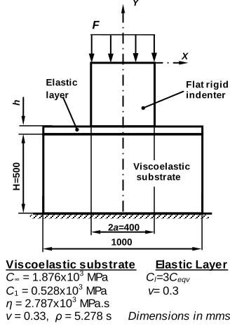
This case study presents a complete analysis of a plane strain frictional nonlinear time-dependent indentation problem. As shown in Fig. 3, a viscoelastic substrate is layered by an elastic layer and indented by a long flat rigid indenter having a width 2a of 400 mm. The layer is assumed to be
H=
500
1000
X Y
Flat rigid indenter
F
Elastic layer
h
2a=400
Viscoelastic substrate
Fig. 3. Indent ation of an elastically layered viscoelastic substrate by a long flat rigid indenter. Viscoelastic substrate Elastic Layer C∞ = 1.876x10³ MPa Cl=3Ceqv
C1 = 0.528x10³ MPa v= 0.3
η = 2.787x10³ MPa.s
v = 0.33, ρ = 5.278 s Dimensions in mms.
perfectly bonded to the substrate. The modulus of elasticity of the layer Cl is assumed to be three times of the viscoelastic equivalent modulus of the substrate Cs, where Cs = C∞+C1, and therefore, a hard layer is considered. The indenter is loaded by a distributed traction F of 10.5 kN/mm. The micro-slip parameter ε and the coefficient of friction µ are 0.75 mm and 0.3, respectively. Due to the symmetry, only a one-half of the problem is modeled. The space domain of the layered substrate is discretized into 1800 four node quadrilateral elements with 1879 nodes. For this indentation problem, indentation pressure, tangential stress, indentation depth and relative tangential displacement at the indentation surface are completely determined. Furthermore, effects of two layer parameters, layer thickness h and layer stiffness Cl, and two interfacial frictional parameters, micro-slip ε and coefficient of friction μ, upon the indentation response are investigated.
A. Effect of the Layer Thick ness
To investigate the effect of the layer thickness upon the frictional indentation response, different layer to substrate thickness ratios h/H of 0.01, 0.02, 0.04, and 0.06 are considered. For all layers Cl/Csof 3 is kept constant, and therefore, hard layering is considered. However, it is important to mention that the effect of the layer thickness is significan tly influenced by the layer stiffness Cl.
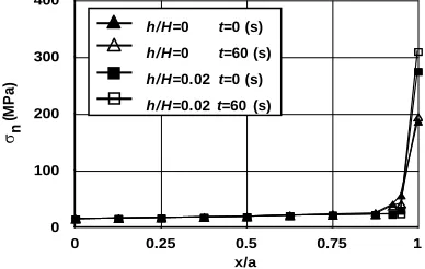
Figure 4 shows the distribution of the indentation pressure
σn along the indentation surface for non-layered h/H=0 and layered substrate h/H=0.02 at the instantaneous and steady state instants of time. It is noticed that the indentation pressure is slightly increased throughout the indentation surface, and then suddenly increased to reach its maximum value at the edges of the indenter. The layer thickness has a considerable effect on the indentation pressure at the edges of the indenter, while this effect is negligible elsewhere. This distribution qualitatively agrees with [31]. Figure 5 indicates that the maximum indentation pressure σn [max], at the two edges of the indenter, increases with increasing of the layer thickness. Due to creep with the time marching, the maximum indentation pressure increases with a constant contact area.
The maximum indentation depth is one of the most important indentation parameters. Figure 6 displays the distribution of the indentation depth un on the top surface of the layer, for non-layered and layered substrate, and at the instantaneous and steady state instants of time. Due to the rigidity of the indenter, the indentation depth has a maximum uniform distribution throughout the indenter contact surface. Such distribution also qualitatively agrees with [31]. Figure 7 indicates that the maximum indentation depth un [max], at the indentation surface, decreases with increasing the layer thickness, even with time marching. These results emphasize that hard layering increases the stiffness of the indented solids, and therefore, decreases the maximum indentation depth. On the contrary, with time marching the creep of the intended viscoelastic solid takes place and the maximum indentation depth increases.
Due to friction, the tangential stress at the indentation surface is also affected by the layer thickness. Figure 8 shows the distribution of the tangential s tress σT throughout the indentation surface, for non-layered and layered substrate, and at the instantaneous and steady state instants of time. Similar to the distribution of the indentation pressure, the tangential stress is almost uniformly distributed throughout the indented surface, and then increased to reach its maximum value at the edges of the indenter. It is noticed that the layer thickness has a considerable effect on the tangential stress at the edges of the indenter. Figure 9 shows that the maximum tangential stress
σT [max], at the two edges of the indenter, increases with the increasing of the layer thickness, even with time marching. This response is due to the increasing of the indentation pressure according to (4).
0 0.02 0.04 0.06
h/H 150
200 250 300 350
n
[
m
a
x
]
(M
P
a
)
Fig. 5. Variation of the maximum indentation pressure with the layer thickness.
t = 0 (s) t = 60 (s)
Fig. 6. Indentation depth distribution at instantaneous and steady state times with two different layer thicknesses.
0 0.5 1 1.5 2 2.5
x/a
-4 -3 -2 -1 0
Un
(
m
m
)
h/H=0 t=0 (s) h/H=0 t=60 (s) h/H=0.02 t=0 (s) h/H=0.02 t=60 (s)
0 0.25 0.5 0.75 1 x/a
0 100 200 300 400
n
(
M
P
a
)
Fig. 4. Indentation pressure distribution at instantaneous and steady state times with two different layer thicknesses.
The distribution of the relative tangential displacement uT at the indentation surface is displayed by Fig. 10. The maximum relative tangential displacement occurs very close to the edges of the indenter. Also, it is noticed that all contact points of the indentation surface experience micro-slipping mode. Figure 11 shows the variation of the maximum relative tangential displacement uT [max] with layer thickness and time. It is clear that uT [max] decreases with the increasing of the layer thickness and increases with time marching. Similar to the indentation depth, this response is attributed to the increasing of the rigidity of the indented solid by increasing the layer thickness, and in turn, reduces the relative tangential displacement. On the contrary, with time marching the creep
of the intended viscoelastic solid is progressing, and therefore, increases the maximum relative tangential displacement.
0 0.02 0.04 0.06
h/H
-4 -3.5 -3 -2.5
Un
[
m
a
x
]
(m
m
)
Fig. 7. Variation of the maximum indentation depth with the layer thickness.
t = 0 (s) t = 60 (s)
0 0.25 0.5 0.75 1
x/a 0
5 10 15 20 25
T
(
M
P
a
)
Fig. 8. T angential stress distribution at instantaneous and steady state times with two different layer thicknesses.
h/H=0 t=0 (s) h/H=0 t=60 (s) h/H=0.02 t=0 (s) h/H=0.02 =60 (s)
0 0.02 0.04 0.06
h/H 5
10 15 20 25
T
[m
a
x
]
(M
P
a
)
Fig. 9. Variation of the maximum tangential stress with the layer thickness.
t = 0 (s) t = 60 (s)
0 0.02 0.04 0.06
h/H 0.1
0.2 0.3 0.4
UT
[
m
a
x
]
(m
m
)
Fig. 11. Variation of the maximum relative tangential displacement with the layer thickness.
t = 0 (s) t = 60 (s)
0 2 4 6 8 10
Cl/Cs 150
250 350 450 550
n
[
m
a
x
]
(M
P
a
)
Fig. 12. Variation of the maximum indentation pressure with the layer stiffness.
t = 0 (s) t = 60 (s)
0 2 4 6 8 10
Cl /Cs
-4 -3.5 -3 -2.5
Un
[
m
a
x
]
(m
m
)
Fig. 13. Variation of the maximum indentation depth with the layer stiffness.
t = 0 (s) t = 60 (s)
0 0.25 0.5 0.75 1
x/a 0
0.1 0.2 0.3 0.4
UT
(
m
m
)
Fig. 10. Relative tangential displacement distribution at instantaneous and steady state times with two different layer thicknesses.
B. Effect of the Layer Stiffness
To investigate the effect of the layer stiffness upon the frictional indentation response, different layer to substrate stiffness ratios Cl/Cs of 1, 2, 3, 4, 6, 8, and 10 are considered. For all layers, h/Hof 0.02 is kept constant. Figure 12 shows the effect of the layer stiffness on the maximum indentation pressure, at the instantaneous and steady state instants of time. It is clear that as the layer stiffness increases the maximum indentation pressure is also increased, however, the maximum indentation depth is decreased, as shown in Fig. 13. On the other hand, increasing of the layer stiffness increases the maximum tangential stress and reduces the maximum relative tangential displacement, as illustrated by Figs. 14 and 15, respectively. With the time marching, the maximum indentation depth is increased due to creep, while the contact area is still unchanged. This in turn increases the maximum indentation pressure and reduces the tendency to the micro -slipping at the indentation surface. Such response increases the maximum values of both the relative tangential displacement and the maximum tangential stress.
C. Effect of the Micro-Slip Parameter
To detect the effect of the micro-slip parameter upon the frictional configuration of the considered indentation problem, different values of the micro-slip parameter ε of 0.5, 0.75, 1.0, 1.25, 1.5, 1.75 and 2.0 mm will be used. For all layers, h/Hof
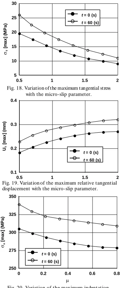
0.02 and Cl/Cs of 3.0, are kept constant. The effect of the micro-slip parameter upon the indentation pressure is depicted in Fig. 16. It is seen that the maximum indentation pressure is increased by increasing the micro-slip parameter. As shown in Fig. 17, the micro-slip parameter of value greater than 1.0 mm does not influence the maximum indentation depth. As illustrated in Figs. 18 and 19, respectively, increasing of th e micro-slip parameter results in decreasing the maximum tangential stress and increasing the maximum relative tangential displacement. This response is due to the reduction of the tangential stiffness, at the indentation surface, with increasing of the micro-slip parameter. This result is also agreed with the adopted local-nonlinear friction model. It is also noticed that the micro-slip parameter has a considerable effect on both instantaneous and steady state values of the maximum indentation pressure and maximum tangential stress. With the time marching, the maximum values of all indentation outcomes are increased due to creep.
D. Effect of the Coefficient of Friction
The coefficient of friction at the indentation surface has a great effect upon the indentation response. To investigate this effect, different values of the coefficient of friction μ ranges from 0.0 to 0.8 are considered. For all layers, h/Hof 0.02 and
Cl/Cs of 3.0 are also kept constant. Variation of the maximum indentation pressure versus the coefficient of friction is presented in Fig. 20. It is found that increasing of the coefficient of friction reduces the maximum indentation
0 2 4 6 8 10
Cl / Cs
5 10 15 20 25
T
[
m
a
x
]
(M
P
a
)
Fig. 14. Variation of the maximum tangential stress with the layer stiffness.
t = 0 (s) t = 60 (s)
0 2 4 6 8 10
Cl /Cs
0.1 0.2 0.3 0.4
UT
[
m
a
x
]
(m
m
)
Fig. 15. Variation of the maximum relative tangential displacement with the layer stiffness.
t = 0 (s) t = 60 (s)
0.5 1 1.5 2
(mm)
250 275 300 325 350
n
[
m
a
x
]
(M
P
a
)
Fig. 16. Variation of the maximum indentation pressure with the micro-slip parameter.
t = 0 (s) t = 60 (s)
0.5 1 1.5 2
(mm)
-4 -3.5 -3 -2.5
Un
[
m
a
x
]
(m
m
)
Fig. 17. Variation of the maximum indentation depth with the micro-slip parameter.
pressure, at both the instantaneous and steady state instants of time. Also, the maximum indentation depth is relatively decreased with increasing of the coefficient of friction, as depicted in Fig. 21. The obtained results are qualitatively agreed with [31] and [32]. In contrast with the distribution of the indentation pressure, the maximum tangential stress is increased with increasing the coefficient of friction, as shown in Fig. 22. This response is due to the direct proportionality between the tangential stress and the coefficient of friction. However, increasing the coefficient of friction considerably reduces the maximum relative tangential displacement, as displayed by Fig. 23. Increasing of the coefficient of friction increases the tangential stiffness, defined by (27). This leads to the reduction of the maximum relative tangential displacement. With the time marching, peaks of all stresses and deformations are increased due to creep of the intended viscoelastic solid.
VI. CONCLUSIONS
Interfacial indentation stresses and deformations of elastically layered viscoelastic solids are significantly influenced by the layer characteristics and the interfacial frictional parameters. A nonlinear time-dependent 2D FE model is exploited to explore the response of frictional viscoelastic indentation problems. Indentation pressure, indentation depth, tangential stress and relative tangential displacement at the indentation surface are determined. Furthermore, effects of layer thickness, layer stiffness, micro -slip parameter and coefficient of friction upon the indentation response are investigated. The frictional indentation response of an elastically layered viscoelastic solid indented by a flat rigid indenter is summarized as follows.
0.5 1 1.5 2
(mm)
5 10 15 20 25 30
T
[
m
a
x
]
(M
P
a
)
Fig. 18. Variation of the maximum tangential stress with the micro-slip parameter.
t = 0 (s) t = 60 (s)
0 0.2 0.4 0.6 0.8
0 10 20 30 40
T
[
m
a
x
]
(M
P
a
)
Fig. 22. Variation of the maximum tangential stress with the coefficient of friction.
t = 0 (s) t = 60 (s)
0 0.2 0.4 0.6 0.8
0.1 0.2 0.3 0.4
UT
[
m
a
x
]
(m
m
)
Fig. 23. Variation of the maximum relative tangential displacement with the coefficient of friction.
t = 0 (s) t = 60 (s)
0.5 1 1.5 2
(mm) 0.1
0.2 0.3 0.4
UT
[
m
a
x
]
(m
m
)
Fig. 19. Variation of the maximum relative tangential displacement with the micro-slip parameter.
t = 0 (s) t = 60 (s)
Fig. 21. Variation of the maximum indentation depth with the coefficient of friction.
0 0.2 0.4 0.6 0.8
-4 -3.5 -3 -2.5
Un
[
m
a
x
]
(m
m
)
t = 0 (s) t = 60 (s)
0 0.2 0.4 0.6 0.8
250 275 300 325 350
n
[
m
a
x
]
(M
P
a
)
Fig. 20. Variation of the maximum indentation pressure with the coefficient of friction.