A Comparison Of Various Machine Learning Algorithms In Designing An Intrusion Detection System

A Comparison Of Various Machine Learning

Algorithms In Designing An Intrusion Detection System

Dr. D. Bhavana, Dr. K. Kishore Kumar, Vishnu Chilakala, Hemanth Gupta Chithirala, Tejesh Reddy Meka

Abstract : The aim of this paper is to effectively utilize the popular machine learning algorithms and train them on the UNSW-NB15 dataset to design a Network Intrusion Detection System (NIDS) based on the algorithm. This system is trained and tested to detect 9 different types of common cyber-attacks as defined in the dataset, namely - Fuzzers, Analysis, Backdoors, DoS, Exploits, Generic, Reconnaissance, Shell code and Worms. This dataset developed in 2015, has 49 varied features for each of the training data and the testing data records. The eventual conclusion would be to compare each of the results on various parameters and understand their limitations and advantages to provide a comprehensive report on each of them.

Index terms: Machine Learning, Intrusion Detection, Network Security, Cyber Security, Cyber-attacks, UNSW – NB15, IDS.

——————————  ——————————

1.

INTRODUCTION

Machine Learning is fast becoming the Industrial Revolution that the present world is so prone to. It is an age-old technology that started gaining traction only recently. Machine Learning dates back to the 1950s when John McCarthy first developed the LISP programming language which is often referred to as the foundation of Machine Learning programming tools used today. The core of this fascinating technology is to design systems that can ‗learn‘ to program themselves for various scenarios, minimizing the need for manual human interventions as far as possible. It has been spreading its wings into many fields like Agriculture, Medicine, Image Processing, Networking, etc. and changing them from the ground up.

1.1 Machine Learning

Machine Learning has two main stages, namely, training and testing. In the training phase, the system is made to ‗learn‘ by providing it with a dataset and an algorithm. Dataset refers to a set of comprehensive, generally huge, data that is used to teach the system. Datasets are one of the integral parts of a machine learning system. It has to be comprehensive and large enough for the system to learn to function under various circumstances. Algorithm is the other important feature which defines ‗how‘ the system is supposed to perceive the provided dataset. The popular, most simple algorithms like Regression, Random Forests, Decision Trees, etc. are being used in various applications. Each algorithm has its own advantages and limitations, which makes the choice of algorithm one of the fundamental steps of developing a machine learning system. In the testing phase, the now-trained system is tested using various data records and the predictions‘ accuracy is used to further train the system, which makes it a continuous and generally iterative process.

1.2 Intrusion Detection System

A Network Intrusion Detection System (NIDS) is a mechanism that is supposed to analyze each request coming and going from the network‘s server to the clients to find the risk of a possible cyber-attack. The 1972 USAF paper written by James P. Anderson [1]is usually cited as the first attempt at developing a network security system. At that point of time, the USAF had the overwhelming job of giving the same level of restricted use of their PC frameworks, which contained different degrees of groupings with each of the clients having varying degrees of system access. This formed the base of another paper written by Anderson in 1980titled ‗Computer Security Threat Monitoring and Surveillance [2] that outlines a network security system to improve computer security auditing and surveillance at customer sites. In August 1985, Dorothy Denning and Paul Neumann pioneered the building of a real-time Intrusion Detection System [3]. This prototype was named the Intrusion Detection Expert System (IDES). This model has been at the core of various enhancements and studies in the network security space, even today. Of the various types of IDS‘, this paper outlines the design of a simple IDS used for anomaly detection.

2. DATASET

The widely used datasets used for designing an IDS are KDDCUP 99, NSLKDD and UNSW – NB15. This paper describes an IDS that uses the UNSW – NB15 dataset due to its significant advantages over the other two [4].

2.1 KDDCUP 99

KDDCUP 99, the upgraded version of DARAP98, has five million connection records with two million connection records for testing. Each record has 41 features along with a class label. The dataset has records regarding 4 different network attacks, namely, Probe, DoS, U2R and R2L. This dataset has been widely used by researchers across the globe due to its availability and comprehensibility. However, three main disadvantages are noted. Firstly, the time to live (TTL) value of packets in the dataset is 126 or 253, whereas most data packets in common network traffic have a general time to live value of 127 or 254. Secondly, the introduction of unfamiliar attack records, which are not available in the training set but are in the testing set, creates a difference between the probability distribution of training set and the probability distribution of testing set. This leads to a prejudice in the system towards the training set‘s attack types, which leads to irregular predictions. ____________________________

 Dr. D. Bhavana, Associate professor ,Department of Electronics and

communication, koneru Lakshmaiah Education foundation,

vaddeswaram,Guntur, A.P,india

 Dr. K. Kishore Kumar, Associate professor, Department of Mechanical

Engineering, koneru Lakshmaiah Education foundation,

vaddeswaram,Guntur ,A.P, india

 Vishnu Chilakala, Hemanth Gupta Chithirala, Tejesh Reddy Meka Graduating students Department of Electronics and communication koneru Lakshmaiah Education foundation,

Finally, the dataset is does not include the more recent types of low footprint network attack projections.

2.2 NSLKDD

After receiving the feedback on the KDDCUP99 dataset and its drawbacks, a new upgraded dataset was created which is referred to as the NSLKDD dataset. The first significant improvement of the NSLKDD dataset over the KDDCUP99 was the removal of duplicate records from the training and testing sets. This reduced the biasing of classifiers towards the repeated records, allowing more accurate predictions. The second advantage is by selecting a wide range of data from a varied range of the KDDCUP99 dataset. This results in the classifiers being trained against a far more diverse range of records. Finally, disposing of the unbalancing problem among a number of records in the training and testing stage to diminish the False Alarm Rates (FARs) is a significant addition over the previous dataset. However, a considerable drawback of NSLKDD is that it is outdated to the present-day low footprint network attacks, which makes it futile to train an IDS for today‘s networks.

2.3 UNSW – NB15

The UNSW – NB15 dataset was released in 2015 by the IXIA Perfect Storm tool in the Australian Centre for Cyber Security (ACCS). The dataset has a total of 175,341 data-entries with a testing set of around 82,000 records from the different types of network interactions. It has 49 features for each record, which are named with descriptions in Table 1. It has data from 9 different network attacks. It is significantly more updated compared to the other two datasets and serves as the base of the IDS described in this paper.

3. NETWORK INTRUSIONS AND IDS

Since Networks are made up of a number of connected devices, they are more prone to cyber-attacks than any other technology. This unauthorized or malicious usage of network is known as a Network Intrusion. To prevent these intrusions, network engineers have pioneered the usage of Network Intrusion Detection Systems (NIDS) and Network Intrusion Prevention Systems (NIPS). There are many IDS and IPS based software available in the market such as Solar Winds Security Event Manager, Snort, OSSEC, Suricata, Bro, Sagan, Security Onion, etc. These aforementioned software at the core of their Security as a Service (SecAAS) companies that provide these services to networks. As we are training our IDS on the UNSW – NB15 dataset, it can detect the 9 types of cyber attacks defined in it. They are Fuzzers, Analysis, Backdoors, DoS, Exploits, Generic, Reconnaissance, Shell-code and Worms[5].

3.1 Intrusion Detection System (IDS)

This paper has simple IDS that are trained using various machine learning algorithms. Since the focus of this paper is to analyze the best algorithm for a machine learning based IDS and not developing the most efficient system, we used a

minimal IDS just for testing out the system‘s accuracy. The concerned system is a network based IDS. It sniffs each of

the data packets traveling in the network for extracts features from it. These features are then sent to the machine learning based model for detecting any abnormalities. If any suspicious model is detected, the system communicates it to the network. This is the perfect example of showing how an IDS works – the most simplistic approach to network security. Since the aim of

the paper is to develop a machine learning based model for IDS, we have trained the system with UNSW – NB15 dataset which can detect 9 different kinds of network intrusions. However, to implement an IDS practically, one has to develop a system that can analyze the data packets and extract features from it to send it to the machine learning based model for any anomaly detection. This paper deals with the latter part of this issue while using a simple IDS as a placeholder for the former.

3.2 Concerned Network Intrusions

The machine learning model developed in this paper is trained with the UNSW -NB15 dataset, which has records concerning 9 different types of network intrusions. They are described in the below subsections.

3.2.1 Fuzzers

Fuzzers is a cyber attack and testing procedure wherein the assailant endeavours to abuse security glitches in an application, working framework or a network by bolstering it with repeated random inputs to crash it.It is a common and simple attack whose model is widely used as a testing technique.

3.2.2 Analysis

Analysis is a network intrusion that aims to penetrate web-based applications via ports, emails and web scripts.

3.2.3 Backdoor

Backdoor is a network intrusion that aims to gain unauthorized access to networks by bypassing an authentication system. This is commonly done remotely using a network connected device to gain access to the secured levels of the network.

3.2.4 DoS

DoS, standing for ‗Denial of Service‘, is a network intrusion that aims to consume all of the computer‘s memory and eventually crash it by sending repeated requests which need to be rejected by the server and thereby taking up memory. It also prevents new devices from hopping on to the network and also disrupts the service to the existing devices. It is a common network attack and one of the most effective.

3.2.5 Exploit

Exploit is a network intrusion that takes advantage of the existing bugs or glitches in the security of a network to cause unintentional, unsuspected behaviour of the network as a whole. It might also lead to an eventual network crash.

3.2.6 Generic

Generic is a cyber-attack that sets up against each cipher block utilizing hash methods to induce a crash irrespective of the configuration of the cipher.

3.2.7 Reconnaissance

Reconnaissance is a cyber-attack where initiator accumulates data about the focused-on PC, which, by and large, goes before a real access or DoS assault.

3.2.8 Shell code

3.2.9 Worm

Worm is a cyber-attack wherein the assailant programs a malware that replicates itself to spread on different PCs on the network. Generally, the extent of the spread is mostly contingent on the security level of the initially targeted system.

4. MACHINE LEARNING AND ALGORITHMS

Machine Learning (ML) is the core technology component of this paper. Using the UNSW-NB15 dataset for training and testing, we are using various popular ML algorithms to train the IDS and comparing the results. This will give a definitive answer of a superior algorithm on a relative level.

4.1 Tensor Flow

This paper uses the commonly used, popular Machine Learning algorithms for training the system. The training has been done using Tensor Flow, which can be accessed from ―https://www.tensorflow.org/‖.Tensor Flow is a free-to-use, open-source programming library. It is a representative math library and is mostly used for machine learning based applications. (akin the IDS we are trying to train.) Tensor Flow was initially engineered by the Google Brain group as a Google internal tool. It was open sourced under the Apache License 2.0 in 2015. Beginning in 2011, Google Brain assembled Dist Belief as a restrictive AI framework dependent on deep learning neural networks. Google allocated various PC researchers to rearrange and re-factor the codebase of Dist Belief into a quicker, progressively robust application-grade library, which became the start of Tensor Flow. Tensor Flow is the Google Brain team's second-age framework. The initial version was released in 2017. Tensor Flow can run on numerous CPUs and GPUs. Tensor Flow is accessible on all major operating systems such as the 64-bit Linux, mac-OS, Windows, and also smart mobile platforms like Android and iOS.

4.2 Algorithms

Machine Learning is a rapidly changing technology today with new advancements being made every day from every corner of the world. While the age old algorithms are still being used, new algorithms that have significant changes over the universally

accepted algorithms are being developed quickly. This paper employs Logistic Regression, Support Vector

Machines, Gradient Boosted Decision Trees, Random Forests and Neural Networks to train the IDS. Each algorithm is used to train the system initially. The system is then sufficiently tested on the testing set of UNSW – NB15 and the results are marked. These results are then compared with each other to reach an eventual conclusion about the best algorithm for training IDS in general.

4.2.1. Logistic Regression

Regression is one of the primal algorithms of ML. It is the base of various algorithms that use regression at varying degrees for predictions. Logistic Regression is one of them and also one of the most used algorithms in Machine Learning in general. Logistic Regression is a machine learning algorithm used for dissecting a dataset in which there is at least one free variable that determines the final predictive outcome. The result is estimated with a binary variable (only two potential results).The main aim of logistic regression is to find the best fitting model that describes the relationship between the binary features of interest (dependent variable refers to the variable that has the final result) and a set of independent (the variables over which

operations are performed to arrive at the resultant variable) variables. Logistic regression generates the coefficients of a formula to predict a logit value of the probability of existence of the desired characteristics:

where p is the probability of the existence of desired characteristics. The logic function is the representation of logged odds as shown below:

and

Estimation in Logistic Regression picks parameters that

augment the probability of observing the sample values. Logistic Regression also uses an Activation Function that is

used to define whether a value belongs to the upper or lower threshold. Generally, sigmoid function is used for activation in Logistic Regression as it approximates a value to one of the two given boundaries. Logistic Regression is a fairly simple algorithm compared to other popular algorithms. It requires minimal human supervision and resources. Input feature tuning and scaling is greatly reduced because of its simplistic approach. The outputs are also well calibrated. However, its simplicity works against itself when it comes to outlier and non-dichotomous data. Also, the chances of misclassification increase with the increasing complexity of data. To conclude, Logistic Regression is a rudimentary approach that is suitable better for simple data.

4.2.2. Support Vector Machines

much you want to avoid misclassifications. For large values of Regularization, the hyper plane margin is constructed in a way to have the smallest margins so that each category is defined to the maximum possible extent. Conversely, for small values, the hyper plane margin is larger and simple which might allow for some misclassifications. Regularization value is directly proportional to processing time i.e. the greater the value, the more time the system takes to generate the hyper plane and get the results. The Gamma parameter simplistically is a measure of the effect of the proximity of points to the hyper plane margin in determination of the hyper plane points i.e. if Gamma is low, even the farthest points from the hyper plane are considered in calculation of the hyper plane. On the other hand, a high Gamma defines to only consider points that are closer to the hyper plane. It has significant impact on the determination of results at a macro level. Margin is a measure of the level of separation to be done between different classes. It is essentially the width of the hyper plane. A big margin shows that the data has been well split into their classes, whereas a small margin shows that the data predictions have been more similar. SVM works relatively better when there is a clear margin of separation between the classes provided in the training data. It is particularly useful compared to other algorithms on data which have more dimensions but not a proportionate number of samples. It is also very memory efficient. However, SVM cannot function on large and diverse datasets. It struggles the most not on the outliers but on the overlapping records of the data, where determining a clear hyper plane between the classes becomes complex. Also, the absence of a clear probability distribution of its predictions brings up problems of its own in time.

4.2.3. Gradient Boosted Decision Trees

Decision Tree is a flowchart-like structure in which each node speaks to a test on an element, each leaf node speaks to a class label, and branches speak to conjunctions of highlights that lead to those class label. The best example to illustrate this would be to consider a coin toss. Each outcome of the toss has a separate node (Heads, Tails) and each of these nodes continue to diversify into even more nodes and branches. It is one of the simplest machine learning algorithms. Decision Trees are is a supervised learning method with no parameters of any kind. It is used for both classification and regression tasks. The model where the final prediction is a set of discrete values is called a Classification tree. Decision trees where the final prediction is continuous information are called Regression trees. These models are generally referred to as Classification and Regression Trees (CART). The level of complexity to be maintained at each node derived from the training data is called Information Gain. It is a measure of the level of information that can be extracted from the features regarding the class itself i.e. it represents a measure of the number of branches coming from each node. The first split will be the one which has the most information gain. This step is repeated until all children nodes are pure, or until the information gain is 0. Boosting is a Machine Learning meta algorithm that is used to amplify a weak learner to become a strong learner. It can an ensemble method that can be applied atop any machine learning algorithm for improving its accuracy. The basic idea of boosting is for each learner to train its weak predecessor. It generally employs a sequential approach. Most boosting algorithms have a model of improving the weak learners iteratively and adding them to a final strong classifier. A weight is assigned to each of the

classifiers, which is generally a measure of its accuracy. When a weak learner is added to a strong learner, the weights are recalculated which results in an overall increase in accuracy. This approach is known as "re-weighting". Re-weighting makes sure that while the misclassified input data has a significant weight gain, the accurate predictions lose weight proportionately. This approach ensures that all the classifiers are weighted, determined as weak or strong, and appropriate approach is followed in the future iterations. There are many Boosting Algorithms like Adaptive Boosting, Gradient Boosting, XG Boosting, etc. each with their own advantages and vices. Gradient Boosting is a type of Boosting algorithm that aims to minimize the errors of each classifier based on its preceding classifier. This approach is employed sequentially. Unlike other Boosting algorithms like Adaptive Boosting, Gradient Boosting aims to fit a new classifier to the residual errors made by the previous classifier. A step by step approach towards Gradient Boosting would be:

1. Create a model and train it with a dataset.

2. Calculate residuals i.e. Actual target value minus the predicted target value.

3. Fit the model to residuals by considering the errors made by the previous classifier.

4. Create a new model by calculating and considering the new weights.

5. As the number of iterations increase, each weak learner is added to a strong learner and the overall accuracy of the model increases.

This approach to Decision Trees is fairly recent and has only been getting popular ever since. It provides greater accuracy compared to other Boosted algorithms or decision trees. Its sequential approach is fairly simple when the accuracy achieved is considered. Also, data preprocessing is greatly reduced in this algorithm as it can handle both categorical and numerical data. However, it is very prone to over fitting as it is a sequential approach. They require lot of resources and time to develop. These tradeoffs might not be feasible for specific applications, as if an error tolerance is significant, there are better algorithms to choose from.

4.2.4 Random Forest

samples. This results in the formation of totally different trees with least correlation. The other method of achieving randomness is Feature Randomness. While general Decision Trees are modeled by considering all available features in the data, Feature Randomness suggests providing a random subset of features to choose from for each tree. This results in an exponential level of randomness for each tree. While any other methods or one of the aforementioned methods can be employed to achieve randomness and decrease correlation between models, using more than one method yields better results and eventual accuracy increase. Random Forest is a great algorithm to use when the dataset is not huge. It can be used for even small number of samples and it yields relatively more accurate results. The use of a number of Decision Trees cancels out the problem of over fitting, as each of the tree‘s fitting levels are countered by the other. They are also very flexible as they can work on all kinds of data with great accuracies. However, their complexity is a main issue when training the system. It requires more resources and time to accommodate the huge model. While it is better at classification, it does a relatively poor job at regression systems as it cannot give precise, continuous predictions. This makes them very prone to over fitting in regression systems. Also, the control over the model is very limited. This makes tuning the model for better accuracy a complex and computationally expensive task. Thus, Random Forest is a better choice where the dataset is not large, and classes are as non-overlapping as possible.

4.2.5 Neural Networks

Artificial Neural Networks (ANN), which are commonly referred to as Neural Networks, are machine learning models inspired by the functioning of the human brain. The model has nodes referred to as ―Artificial Neurons‖ and each neuron is connected to the others and influence it. The network also has various layers of neurons. These layers are generally expected to be the sub problems of the whole computation. If the network has a greater number of layers, typically 2-8, the network is referred as a Deep Neural Network (DNN).Thus, the final prediction is a summarization of the various changes that occur while processing the data through the network. Warren McCulloch and Walter Pitts published a paper in 1943[6] that is widely accepted to have started the conversation of the creation of artificial neural networks. Around the same time, D. O. Hebb created a new learning hypothesis called Hebbian Learning. These authors are credited to be the pioneers of ANN modeling. A neuron is defined to have two states – activeor fired, and in activator not fired. Each neuron has a Weight that changes according to the inputs given to it. Every neuron has two parameters, namely, a threshold value and an activation function. A threshold value is the minimum amount of weight required to be given to a neuron to activate it. The activation function refers to any computation that is needed to be done to the incoming weights before thresholding it. These parameters are responsible for all the changes that occur in the neural

network and are responsible for the final predictions. The activation of each neuron depends on the input weights it

gets from other neurons. If the function of the incoming weights is greater than its Threshold, the neuron is said to be activated. This function that influences the weights is Activation Function. These activation functions must be as computationally efficient as the number of neurons on the network. The three main types of activation functions are Binary Step functions, Linear

Activation functions and Non-Linear Activation functions. Each one of them have their own advantages and vices, and a preference must be made after carefully studying the application for which the model is to be employed. Sigmoid, Hyperbolic, Rectified Linear Unit (ReLU), Softmax, Swish, etc.

are the common activation functions used in ANN. In Neural Networks, information is stored and processed over

the entire stretch of the network. This makes sure that the processing as a whole does not stop if any data is missing. It has a great fault tolerance, owing to its decentralized approach. It can also process information parallelly, reducing processing time to great lengths. However, they are hugely dependent on the hardware and require great processing powers to function. Also, the decentralized approach prevents easy locating of any errors in the network. It provides no information as to its approach towards the problem. In conclusion, while Neural Networks offer great accuracies and function even with irregular data, their huge computational needs and long training times means they can only be applied to specific applications.

4.2.6 Convolution Neural Networks

5. RESULTS

This section summarizes the final results of our research. For every algorithm, the IDS is trained from scratch and is tested again on the UNSW – NB15 dataset. This unbiased, clear approach made sure that each algorithm‘s accuracy is unaffected in any way by the previous test. All the models have been trained on Google‘s Tensor Flow platform.

5.1 Logistic Regression

The IDS has been trained with Logistic Regression for 10000 epochs. The status has been noted for every 500 epochs, as shown in Figure 1.

Figure 1

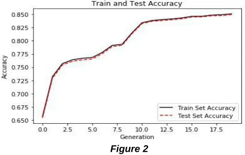
From the above mentioned results, it can be inferred that as the number of epochs increases, the accuracy of the model increases. The accuracy stays largely unchanged on the testing set compared to the training set, as shown in Figure 3. The final accuracy after training the system for 10000 epochs is 84.9551%, which can be approximated to 85%.

Figure 2

5.2 Support Vector Machine

This model has been trained by employing the SVM algorithm. It has been trained for 10000 steps with a zero bias weight to get the most natural results, The results are shown in Figure 3.

Figure 3

As shown in the above figure, the model has been trained for 10000 steps and the final result is shown. It achieves an accuracy of 89.55137%, which can be approximated to 90%.

5.3 Gradient Boosted Decision Trees

This model has been trained using the Decision Trees algorithm by employing Gradient Boosting on top of it. It has been trained for 603 steps and the final results are shown in Figure 4.

Figure 4

As shown in the above figure, the model achieves an accuracy of 94.8384%, which can be approximated to 95%.The model also has a precision of 96.317%.

5.4 Random Forest

This model has been trained by employing the Random Forest algorithm, It has been trained for 1000 steps with a result at every 500 steps as shown in Figure 5.

The above mentioned results show that the model achieved an overall accuracy of 54.6728%, which can be approximated to 55%.

5.5 Neural Networks

This model has 3 hidden layers with 50,100 and 50 neurons in each of them. It uses ReLU and Softmax activation functions over 10 epochs to determine the results as shown in Figure 6.

Figure 6

As shown in the above figure, the model achieves an accuracy of 93.05% which can be approximated to 93%.

5.6 Convolution Neural Networks

This model has 7 layers, each having a ReLU activation function. They are followed with pooling layers and are enveloped by the input and output layers. This model has then been trained for 10 epochs and the results are as shown in Figure 7. As shown in the below figure, the model achieves an accuracy of 93.27%, which can be approximated to 93%.

Figure 7

6. COMPARISON

All the results mentioned in the previous section can be summarized as shown below in Table 1.

TABLE 1

COMPARATIVE TABLE ON DIFFERENT ALGORITHMS

S. No. Algorithm Accuracy

1. Logistic Regression 85% 2. Support Vector Machine 90% 3. Gradient Boosted

Decision Trees 95%

4. Random Forest 55%

5. Neural Network 93%

6. Convolutional Neural

Network 93%

7. CONCLUSION

As can be concluded from the above results, Gradient Boosted Decision Trees provided the most accurate predictions on the UNSW – NB15 dataset. Ignoring the effect of the number of iterations, this algorithm can be concluded to be the best among the aforementioned four algorithms to develop an IDS. The next best would be to use Neural Networks to program the system.

7. REFERENCES

[1] Anderson, James P. "Computer security threat

monitoring and surveillance." Technical Report, James P. Anderson Company (1980).

[2] Anderson, James P. Computer Security Technology

Planning Study. Anderson (James P) and Co Fort Washington PA, 1972.

[3] Denning, Dorothy, and Peter G.

Neumann. Requirements and model for IDES-a

real-time intrusion-detection expert system. SRI

International, 1985.

[4] Moustafa, Nour, and Jill Slay. "UNSW-NB15: a

comprehensive data set for network intrusion detection systems (UNSW-NB15 network data set)." In 2015 military communications and information systems

conference (MilCIS), pp. 1-6. IEEE, 2015.

[5] Moustafa, Nour, and Jill Slay. "The significant features

of the UNSW-NB15 and the KDD99 data sets for network intrusion detection systems." In 2015 4th international workshop on building analysis datasets and gathering experience returns for security (BADGERS), pp. 25-31. IEEE, 2015.

[6] McCulloch, Warren S., and Walter Pitts. "A logical