Simulation Study of Alfv´en-Eigenmode-Induced Energetic Ion
Transport in LHD
∗
)
Seiya NISHIMURA, Yasushi TODO, Donald A. SPONG
1),
Yasuhiro SUZUKI and Noriyoshi NAKAJIMA
National Institute for Fusion Science, Toki 509-5292, Japan
1)Oak Ridge National Laboratory, Oak Ridge, Tennessee 37831, USA
(Received 22 November 2012/Accepted 22 April 2013)
The interaction between toroidal Alfv´en eigenmode (TAE) and energetic ions in the Large Helical Device (LHD) is investigated using a reduced version of the MEGA code that implements a realistic equilibrium magnetic field with the HINT code and corresponding TAE profile with the AE3D code. In simulations, the linear growth rate of TAE amplitude is proportional to energetic ion density; consequently, the nonlinear saturation level of the TAE amplitude is enhanced by the increase in the energetic ion density. Energy transfer analysis is performed to clarify destabilization and saturation mechanisms of the TAE and to identify resonant energetic ions. An analysis of test particles in the electromagnetic field perturbed by the TAE shows that the magnitude of fluctuations in the energetic ion orbits is proportional to the square root of the TAE amplitude. Our results qualitatively reproduce the radial transport of energetic ions by the TAE in the LHD.
c
2013 The Japan Society of Plasma Science and Nuclear Fusion Research
Keywords: Alfv´en eigenmode, energetic ion, three-dimensional equilibrium, hybrid simulation, particle-in-cell method
DOI: 10.1585/pfr.8.2403090
1. Introduction
To achieve magnetic confinement fusion, the interac-tion between Alfv´en eigenmodes and energetic ions is an important issue to be resolved [1]. In the Large Helical De-vice (LHD), which is a stellarator, bursts of toroidal Alfv´en eigenmode (TAE) and associated energetic ion transport and losses have been observed during neutral beam injec-tion [2]. TAE-induced energetic ion transport has been in-vestigated in axisymmetric systems such as tokamaks [3], but that in stellarators relies on an analogy with tokamaks and is not yet fully described. In this paper, we approach this problem using areducedversion of the MEGA code [4–6]. In this code, data from the HINT code [7, 8], which solves the resistive magnetohydrodynamic (MHD) equa-tions, is used to obtain the realistic equilibrium magnetic field in the LHD. The TAE spatial profile in the equilib-rium field is given by the AE3D code [9], which solves the reduced MHD equations for stellarators [9–11]. The energetic ion orbits in the superposition of the equilibrium and perturbed fields are calculated by the particle-in-cell method with the so-calledδf method [12]. Using the code, the time evolution of the TAE amplitude and the conse-quent energetic ion transport in the LHD are simulated.
This paper is organized as follows. In§2 and§3, we briefly introduce the simulation model. In§4, the linear growth rate of the TAE and the nonlinear saturation level
author’s e-mail: [email protected]
∗)This article is based on the presentation at the 22nd International Toki
Conference (ITC22).
of the TAE amplitude are surveyed. In§5, the magnitude of the fluctuation in energetic ion orbits due to the TAE is investigated by test particle analysis. Finally, a summary is presented in§6.
2. Data from HINT and AE3D Codes
The HINT code and AE3D code employ the Boozer coordinates (ρψ, ϑ, ζ) are employed, whereρψ∝ √ψtis the
normalized minor radial position, ψt is the toroidal
mag-netic flux,ϑis the effective poloidal angle, andζis the ef-fective toroidal angle. In the MEGA code, data described by the Boozer coordinates are converted to the cylindrical coordinates (R, φ,Z), whereRis the major radial position, φis the toroidal angle, andZis the vertical position.
Figure 1 shows (a) the poloidal cross section of the equilibrium magnetic field in the LHD at different toroidal angles,φ =0 [rad] andφ =π/10 [rad], and (b) the radial profile of the rotational transform. In the LHD, helically wound coils have a pole number (symmetry number in the poloidal direction) ofl=2 and a pitch number (symmetry number in the toroidal direction) ofM =10. The average minor radius is approximatelya = 60 [cm]. Because the AE3D code requires a nested magnetic surface, the VMEC code [13] is also used to construct the nested equilibrium magnetic field which is comparable to that in Fig. 1.
Figure 2 shows the Alfv´en continua of the n = 1 mode family calculated by AE3D. Many eigenmodes are observed in Fig. 2, but we focus on the TAE withn = 1 andm = 0,1,2,and 3 for the reduced simulation, which
c
2013 The Japan Society of Plasma
Fig. 1 Equilibrium magnetic field in LHD calculated by the HINT code: (a) Poincar´e plots of equilibrium magnetic field at toroidal anglesφ=0 [rad] andφ=π/10 [rad] and (b) radial profile of rotational transform in the Boozer co-ordinates.
Fig. 2 Alfv´en continua ofn = 1 mode family calculated by AE3D.
corresponds to the slowly changing bold curves, wheren
is the toroidal mode number andmis the poloidal mode number.
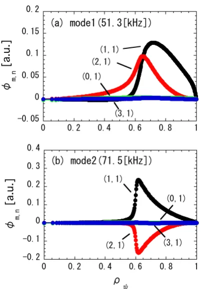
Figure 3 shows the radial profile of the electrostatic potential of the TAE for modes with frequencies of (a) 51.3 [kHz] and (b) 71.5 [kHz]. In both modes, (m,n) = (1,1) and (m,n) = (2,1) are dominant. Those modes are located inside the continuum gap owing to the toroidal cou-pling of the (1,1) and (2,1) modes. In AE3D, the boundary condition with the perfect conductor is used [9]; that is, the
[a.u.]
[a.u.]
Fig. 3 Radial profile of the electrostatic potential of TAE cal-culated by AE3D for modes with frequencies of (a) 51.3 [kHz] and (b) 71.5 [kHz].
electrostatic potential perturbation is zero atρψ=1, which might give rise to rapid radial decay of 51.3 [kHz] (1,1) mode at the edge boundary.
The rotation frequency of the shear Alfv´en wave is given byωm,n =±km,nvA, wherekm,n =(1/R0)(mι−n) is
the parallel wave number,R0is the major radial position of
the magnetic axis,vAis the Alfv´en velocity, and the sign
indicates the direction of propagation. The resonance con-dition,ω1,1 = −ω2,1 determines the center of the gap as
ι=2/3 at the radial position ofρψ =0.65 [see Fig. 1 (b)], which is close to the peaks of the eigenfunctions in Fig. 3. Aroundρψ = 0.65, a gap in the eigenfrequency forms, where the frequencies at the lower and upper accumulation points are 49.5 [kHz] and 72.0 [kHz], respectively.
3. Simulation Model
The nonlinear energetic ion dynamics are determined by the electromagnetic field, which is the sum of the equi-librium field and TAE perturbation. The energetic ions are represented by marker particles, and the electromagnetic field at the particle position is given by the particle-in-cell method with linear interpolation.
The time evolution of the guiding center velocity of energetic ions,ugc, is determined by the drift-kinetic
drift velocity),E×Bdrift velocity, curvature drift velocity, and∇Bdrift velocity:
ugc=u∗+uE∗+u∗c+u∗B
=vB
B∗ b+
1
B∗E×b+
ρvB
B∗ ∇ ×b
− μ
qepB∗∇
B×b. (1)
The original velocity parallel to the magnetic field line,v, obeys the evolution equation:
mep
dv dt =
B∗
B∗ ·
qepE−μ∇B
, (2)
where E is the electric field, b is the unit vector of the magnetic field, Bis the magnitude of the magnetic field,
B∗ = B(1+ρb · ∇ ×b) is the magnitude of the eff ec-tive parallel magnetic field, ρ = mepv/qepB is the
par-allel Larmor radius,μ = mepv2⊥/2B2 is the magnetic
mo-ment,mepis the energetic ion mass,qepis the charge, and
v⊥ is the perpendicular velocity. The equilibrium ener-getic ion distribution function f0 is modeled by coupling
the Gaussian, and slowing-down distributions [15] such that f0 ∝ exp (−ρ2ψ/δρ2ψ)/(v3+v3c)erfc((v−v0)/δv), where
vis the absolute value of the energetic ion velocity and the complementary error function is defined as erfc (s) = (1/√π)s∞exp−t2dt, wheresis arbitrary. In the
simu-lations, we chooseδρψ =0.4,vc/vA =0.5,v0/vA =1.18,
andδv/vA = 0.1. The numerical factor of f0 is specified
when we choose the energetic ion density at the plasma center. The initial distribution of the pitch angle parameter λ=v/vis assumed to be isotropic inv−v⊥space, where v= v2
+v2⊥.
The electric field and the magnetic field perturbed by the TAE are given by E = Ec +Es = −∇⊥(Φs+Φc)
and B = B0 +∇ ×
As+Ac
b , respectively, where B0 is the equilibrium magnetic field given by the HINT
code. The sine and cosine components of the electro-static potential perturbation and the parallel vector poten-tial perturbation are modeled byΦs = Xm,nφm,nsinΘ,
Φc=Ym,nφm,ncosΘ,As=Xm,nam,nsinΘ, andAc=
Ym,nam,ncosΘ, respectively, whereΘ=mϑ−nζ−ωt,ω
is the eigenfrequency given by AE3D,{φm,n,am,n}are the
eigenfunctions given by AE3D, and {X,Y} are the time-dependent amplitudes. The rate of increase in the ener-getic ion energy is given byjep·E, where jepis the en-ergetic ion current due to the curvature drift and∇Bdrift, and the bracket indicates the volume integral. In theδf
method, the volume integraljep·Eis calculated by sum-ming each particle’s contribution multiplied by a weight function [4, 12]. The weight function is defined as the product of the distribution function perturbation and the phase-space volume filled by each particle, and the evolu-tion equaevolu-tion of the weight funcevolu-tion is based on the per-turbed Vlasov equation. The stored energies of the sine
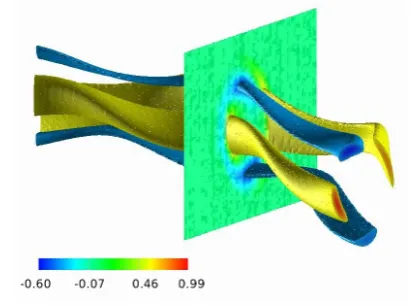
Fig. 4 Contour and isosurface plots of the electrostatic potential of the TAE by the AE3D code implemented in the MEGA code (arbitrary units).
and cosine components of the TAE,Ws andWc, are
pro-portional toX2andY2, respectively. Then, the energy
con-servation law yields the following relations 1
X
dX
dt =−
1
Ws
jep·Es, (3)
1
Y
dY
dt =−
1
Wc
jep·Ec. (4)
Figure 4 shows the implementation of the TAE data by the AE3D code in the MEGA code. An example of a contour plot of the electrostatic potential of the TAE in the poloidal plane and isosurface plots are shown. Note that the rippled structure in Fig. 4 is due to the helically wound equilibrium magnetic field.
In the following simulations, the number of marker particles is 6.6×10⁵, and the pitch angle parameterλof
each marker particle in the initial distribution is determined by a pseudo random number generator.
4. Simulation Results
The plasma parameters for the following simulations areBeq=0.5 [T] andneq=8.9×10¹⁸[m−3], whereBeqis
the maximum toroidal magnetic field andneqis the
maxi-mum plasma density.
-
Fig. 5 Dependence of the linear growth rate of the TAE on the energetic ion density at the plasma center.
eq
eq
eq
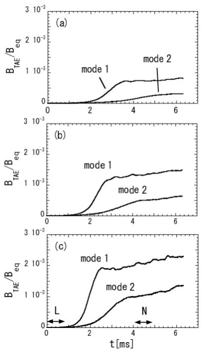
Fig. 6 Time evolution of TAE amplitude with different values of the energetic ion density at the plasma center: (a) 3× 10¹⁷[m−3], (b) 4×10¹⁷[m−3], and (c) 5×10¹⁷[m−3].
sensitive to the values ofvcandδv.
Figure 6 shows the time evolution of the TAE ampli-tude, where the maximum amplitude of the magnetic field due to the TAE perturbation is represented by BTAE. In
the early phase, exponential growth of the mode amplitude is observed. The TAE growth enters the nonlinear phase
Fig. 7 Parallel energetic ion velocity spectrum of energy transfer from energetic ions to the low frequency TAE (mode1) in the (a) linearly growing regime and (b) nonlinearly growing regime, corresponding to Fig. 6(c), whereE0 =
85.1 [J] is a normalization parameter.
when the mode amplitude becomes sufficiently large. The saturation amplitude increases monotonically with the en-ergetic ion density. The oscillatory behavior of the mode amplitude in the saturation phase is due to particle trap-ping by the TAE, which interrupts the energy exchange among particles and waves, giving rise to the saturation of the mode growth [16]. In fact, the oscillation of the mode amplitude in the saturation phase in Fig. 6 has a time scale on the order of 1 [ms], which is of the same order as the linear growth rate of the TAE. After the first nonlinear sat-uration, the mode growth gradually continues. It is also confirmed that the TAE frequency does not vary by more than the linear growth rate of the TAE, which is consistent with the constraints imposed by the constant mode struc-ture and equilibrium. In other words, the mode growth rate is much smaller than the mode frequency; thus, the feed-back to the mode frequency is negligible.
To identify resonant energetic ions, which drive the linear and nonlinear growth of the TAE, we analyze the energy transfer process. Considering Eqs. (3) and (4), the energy transfer from energetic ions to the TAE is given by − dtjep·(Es+Ec).
μ
μ
Fig. 8 Parallel energetic ion velocity and magnetic moment spectrum of energy transfer from energetic ions to the low-frequency TAE (mode 1) in the (a) linear growth regime and (b) nonlinear growth regime, corresponding to Fig. 6(c), where the energy is normalized by E0 =
85.1 [J].
parallel velocity close to v = 0.6 [vA] drive the linear
growth of the TAE. In the nonlinear (N) regime, the en-ergy transfer aroundv = 0.6 [vA] tends to be cancelled
out, which might be due to particle trapping caused by the TAE-induced electric field. However, energetic ions with a parallel velocity close tov =0.3 [vA] and 0.8 [vA] newly
drive the nonlinear growth of the TAE.
Figure 8 shows the parallel energetic ion velocity and magnetic moment spectrum of energy transfer to the low-frequency TAE in regimes L and N. Figures 8 (a) and (b) correspond to Figs. 7 (a) and (b), respectively. Figure 8 in-dicates that the resonance parallel velocity depends on the magnetic moment.
Figures 7 and 8 clarify that the gradual growth of the TAE in the nonlinear regime is caused by the shift in the energy source. The trapping of resonant energetic ions with the resonant parallel velocity, vres , implies that the TAE-induced field is strong enough to deform the orbits of energetic ions with parallel velocities close tovres
. Then, the modification of the energetic ion orbit enables the TAE to access a new energy source and triggers nonlinear in-stability. However, the mechanism of the access to the new energy source is not yet fully understood in detail, although it might be investigated elsewhere. If the inherent damp-ing of the TAE modes is included in Eqs. (3) and (4), it will dominate the weak nonlinear instability observed in our simulation.
TAE/B TAE/B
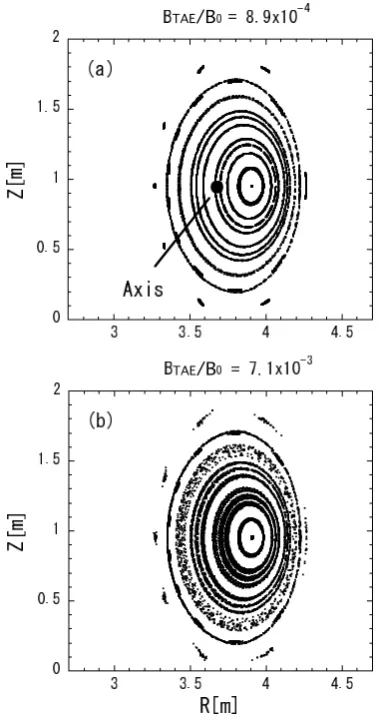
Fig. 9 Poincar´e plot of test particles in vertically elongated poloidal planes for (a) BTAE/Beq = 8.9×10⁻⁴ and (b)
BTAE/Beq=7.1×10−3.
5. Test Particle Analysis
In the following, we perform the test particle analysis to clarify the energetic ion orbit. The simulation conditions are as follows: the number of test particle is 102, and the
initial particle velocity isv = v0 = 1.18vA andv⊥ = 0;
only the low-frequency mode (mode 1) is considered, and the amplitude of the TAE is fixed but the TAE is oscillated with the linear rotation frequency.
Figures 9 and 10 show Poincar´e plots of the test parti-cles in the vertically elongated plane (φ =kπ/5 [rad]k=
0,1,2, ..., 9) and the horizontally elongated poloidal plane (φ = π/10+kπ/5 [rad]k = 0, 1, 2, ..., 9), respectively for different values of the TAE amplitude. The axis of the equilibrium magnetic field is shown in Figs. 9 (a) and 10 (a). In comparison with Fig. 1 (a), it is observed that the orbit strongly deviates from the magnetic surface owing to the curvature drift. Note that the∇Bdrift is absent because only test particles withv⊥ =0 are used, and the condition μ=0 holds in the simulation.
TAE/B TAE/B
Fig. 10 Poincar´e plot of test particles in horizontally elongated poloidal planes for (a)BTAE/Beq = 8.9×10⁻⁴ and (b)
BTAE/Beq=7.1×10−3.
Fig. 11 TAE amplitude dependence of the maximum orbit width of test particles in the horizontally elongated and the ver-tically elongated planes.
maximum orbit width is measured on the interior equato-rial plane. The orbit width in the horizontally elongated plane is approximately 1.6 times of that in the vertically elongated plane. This factor roughly agrees with the as-pect ratio of the semi-major axis to the semi-minor axis in
the poloidal cross section,∼1.8, which indicates that the change in the orbit width is due to the toroidal dependence of the magnetic surface shape.
For our simulation condition, we conclud that the or-bit width is approximately 10% of the average minor ra-dius when the TAE amplitudeBTAE/Beqis in the range
be-tween 10−3and 10−2, which is consistent with the results in Ref. [5], using an axisymmetric equilibrium magnetic field comparable to that of the LHD. In LHD experiments, the radial transport of energetic ions sometimes reaches 10% of the average minor radius [2]. A comparison with ex-perimental data is necessary to check the validity of our results; this is left as a future work.
6. Summary
In this study, the interaction between the TAE and en-ergetic ions in a realistic equilibrium magnetic field in the LHD was investigated. In the linear growth phase of the TAE, the linear growth rate is proportional to the energetic ion density. In the nonlinear simulations, the saturation level of the TAE amplitude increased with the energetic ion density. Energy transfer analysis identified the reso-nant energetic ions, which drive the linear instability, first saturation, and nonlinear instability of the TAE. A test par-ticle analysis showed that the magnitude of the fluctuation of energetic ion orbits is proportional to the square root of the TAE amplitude. Simulations of more realistic sit-uations with neutral beam injection and the finite plasma pressure effect are left as future works.
Acknowledgements
Numerical computations were performed at the Helios at the IFERC-CSC and the Plasma Simulator at the Na-tional Institute for Fusion Science. This work was partially supported by a Grant-in-Aid for JSPS Fellows (23-5218).
[1] W.W. Heidbrink, Phys. Plasmas15, 055501 (2008). [2] M. Osakabeet al., Nucl. Fusion46, S911 (2006).
[3] W.W. Heidbrink and G.J. Sadler, Nucl. Fusion 34, 535 (1994).
[4] Y. Todoet al., Phys. Plasmas10, 2888 (2003). [5] Y. Todoet al., Plasma Fusion Res.3, S1074 (2008). [6] Y. Todoet al., Fusion Sci. Technol.58, 277 (2010). [7] K. Harafujiet al., J. Comput. Phys.81, 169 (1989). [8] Y. Suzukiet al., Nucl. Fusion46, L19 (2006). [9] D.A. Sponget al., Phys. Plasmas17, 022106 (2010). [10] S.E. Krugeret al., Phys. Plasmas5, 4169 (1998). [11] O.P. Fesenyuket al., Phys. Plasmas9, 1589 (2002). [12] A.Y. Aydemir, Phys. Plasmas1, 822 (1994).
[13] S.P. Hirshman and J.C. Whitson, Phys. Fluids 26, 3553 (1983).
[14] R.G. Littlejohn, J. Plasma Phys.29, 111 (1983).
[15] J.G. Cordey and M.J. Houghton, Nucl. Fusion 13, 215 (1973).
[16] H.L. Berk, B.N. Breizman and M. Pekker, Phys. Rev. Lett.
76, 1256 (1996).