APPLING GREY FORECASTING METHOD TO FORECAST THE PORTFOLIO’S RATE OF RETURN IN STOCK MARKET OF IRAN

APPLING GREY FORECASTING METHOD TO FORECAST THE PORTFOLIO’S

RATE OF RETURN IN STOCK MARKET OF IRAN

Ali Mohammadi, Sara Zeinodin Zade Shiraz university, Shiraz, Iran E-mail: [email protected]

ABSTRACT

Stock market is one of the most important investment market, which influenced by many factors, therefore it needs a robust and accurate forecasting. In this study ,grey model used as a forecasting method and examined if it is the most reliable forecasting method in comparison of time series method. The information of portfolio’s rate of return is gathered from 50 accepted companies in Tehran stock market, which were announced as the best companies last year. Mean Square of the errors (MSE) is computed by different value of α in grey model which could be varied between .1 to .9 ,to examined if α=.5 is the best value that our model could take .Then the predictive ability of the model is compared with different type of time series based forecasting methods Experimental results confirm forecasting accuracy of grey model. Tracking signal is computed for grey model to see whether grey model forecasting is in control or not. At the last portfolio’s rate of return is forecasted for next periods.

Keywords: Grey model, Stock market, Forecasting, time series

1. INTRODUCTION

In general, people are highly interested in forecasting future tendency of some events, such as investment in stock market, which is necessary to be forecasted for obtaining higher profit and reducing the investment risk. Since the prediction is mainly used to reduce the uncertainty or risk in marketing decisions ,therefore prediction accuracy is crucial.

How to select an appropriate and accurate method to predict the output forecast for enterprises is a problem of highest importance. Consequently, a method with low cost and high accuracy of the prediction has always been the goal of management decision-maker.

In recent years, researchers have developed various quantitative forecasting methods. Even though there are many forecasting methods, there does not exist a method with predictive accuracy in all circumstances.

Unfortunately, the traditional prediction model often needs to meet with large number sample or normal distribution that cannot be used to short term forecasts. In recent years, to overcome these limitations, artificial intelligence was introduced to amend traditional forecasting methods. Artificial intelligence including the artificial neural network (Hsieh,Hsiao & Yeh, 20011; Ebrahimpour, Nikoo, Masoudnia Yousefi &Ghaemi,2010),fuzzy theory(Chen,Cheng &Teoh 2008),Neural-Fuzzy system(Atsalakis &Valvanis,2009), Markov-Fourier Grey model (Hsu,Liu,Yeh &Hung ,2009) are used to solve traditional forecasting problems .

The grey theory applies to the concern of sample of small data, in which systems for the “uncertainty” , “multi-input” , “discrete data” , and” incomplete data” can effectively be addressed. It fit well with today’s fast-changing industrial environment. Hence the current study proposed grey model, for assisting investors in predicting the future behavior of stock market and help them to make a rational decisions.

The grey system theory was proposed by Deng (1982). The grey model (GM) is one of the best feature in grey system theory. Generally, the grey model is written as GM(m,n) , where m is the order and n is the number of variable of the modeling equation . GM(1,1) is the most widely used and is successfully demonstrated in many application.

of the models are compared with different type of forecasting in time series, which here is Naive method, Simple Average, Moving Average, Single Exponential Smoothing.

The reset of this paper is organized as follows. section 2 describes grey model which is used as a forecasting method in stock market. Section 3 presents the results and compares of the proposed model with α=.5 and the other value of α, and compares of grey model accuracy with time series forecasting method and also results of tracking signals which are computed for grey model, and at the last of this section future return rate is forecasted . section 4 summarized the findings.

2. METHODOLOGY

The procedure of the original GM(1,1) model will be briefly illustrated in the following.

Assume that stands for the raw data series of portfolio’s rate of return ,namely,  



_x 

_{ }

_x 

_{ }

_x 

_{ }

_x 

_{ }

_n



x   1,  2,  3,...,  (1)

Where n is the sample size. By 1-AGO(one time Accumulated Generating Operation) ,the preprocessed

series,

 



_x 

_{ }

_x 

_{ }

_x 

_{ }

_x 

_{ }

_n



x1  1 1, 1 2, 1 3,..., 1 (2)

Where

x

 

 

k

k

x

 

 

m

for

k

n

m1

,

1

,

2

,...,

1











By mean operation on ,the series

Where Z(1) (Z(1)(1),z(1)(2),...,z(1)(n)) (3)

Thus ,from grey system theory (Deng,1988)the grey differential equation of GM(1,1) and its whitening equation are obtained, respectively, as follows:

 

_{ }

 

_{ }

n

k

b

k

aZ

k

x

0



1



,



2

,

3

,...,

   

b

ax

dt

dx

_

1

_

1

(4)

Where a and b is the developing coefficient and grey input, respectively. Let be the parameters vector. By

using least squares method (Hsia,1979), the parameters a and b can be obtain as





         b a Y X X

XT 1 T

ˆ  (5) Where  

_{ }

 

_{ }

 

_{ }

 

_{ }

 

_{ }

 

_{ }

_                                n X X X Y n Z Z Z X 0 0 0 1 1 1 3 2 1 1 3 1 2    (6)

And x denotes the accumulated matrix and Y represent the constant vector. The approximate relation can be

obtained by substituting the into the differential equation, and solving equation (4)

 

_

_

 

_{ }

a b e a b X k

xˆ1 1 _  1  _ ak

(7)

Where (1)= (1) . by IAGO (inverse AGO) equation (7) the recovered value (k) is:

 

_{ }

 1

_{ }

 1

_

_





 

_{ }

 1

1 1 1 ˆ ˆ ˆ       _    

 a ak

e a b x e k x k x k

x 

(8)

Given k=1,2,3,….n, the predictive value is  



_x

_{ }

_x 

_{ }

_x 

_{ }

_x 

_{ }

_n



xˆ  ˆ1 , ˆ 2 , ˆ 3 ,..., ˆ (9) Finally, the forecasting data is further examined to see if it meets the residual error checking procedure. Usually,

 

  

 

_{ }

_{ }

ˆ 

 

100%

k x

k x k x k

e _

 

(10)

But because in this case, the value of some raw data is zero, we use the square sum of the errors for comparing the errors as below:

 

 

 

 

 

 

   

 

   

 

   

 

   

 

 

n n

s

T

T

  

  

 

 

3 2

. 3 2

(11)

3. EMPIRICAL ANALYSIS

In order to show the predictive ability of GM (1,1) model, its performance and comparison with other models(time series),we choose the Tehran stock market as a sample.

We use the information of portfolio’s rate of return in 50 accepted firms in Tehran stock market. This information is gathered from March 2007 to February 2010 .

Some information of some company was missed. And we could just gather information of 45 company.

3.1.Diffrent value of back ground

At first we compute mean square of errors of grey model by different value of α , which could differ between .1 to .9(.1<α<.9). α is called generation coefficient (or weight). When α>.5 the generation is said to have “emphasis more on new and less on old information “. When α<.5, the generation is said to have “emphasis more on old and less on new information”. And when α=.5, the generation we get the best result.(liu & lin,2006) Mean square of errors computed by different value of α which started from .1,the procedure stops whenever errors increase in comparison of last error value which computed with lower value of α. By this way we can be sure that, α=.5 gives us the best results and the most accurate model. The results are shown in table 1.

Firm α=.1 α=.2 α=.3 α=.4 α=.5 Α=.6

A 9961.2 9954.4 9949.2 9945.7 9943 9943.6

B 3120.9 3119.2 3118.3 3117.6 3117.5 3118

C 4745.9 4744.2 4742.7 4742 4740 4742

D 2695.3 2694.4 2693.7 2693.2 2690 2693.2

E 3543.1 3541.9 3508 3540 3570

F 3055 3054 3053.2 3052.8 3052 3052.8

G 3395.3 3393.9 3392.5 3391.7 3391.1 3390.9

H 5010.9 5008.9 5007.1 5006.3 5005 5006.3

I 3698.2 3702.1 3706.5 3716

J 25893 25879 25871 25867 25867 25872

K 3448.8 2447.7 3446.9 3446.5 3440 3446.4

L 6326.5 6307.6 6312.3 6324.8

M 3565.6 3564.3 3563.9 3564.2 3565.6

N 544.10 543.00 542.30 541.78 541.51 541.52

O 4719.2 4716.9 4715.2 4714.2 4713.8 47140

P 4671 4666.9 4663.8 4661.6 4660 4660

Q 1190.2 1192.4 1200

R 4335.9 4334.2 4332.7 4332 4260 4331.9

S 7308.8 7304.3 7300.7 7298.8 7298 7299.1

T 5250.5 5248 5246.3 5245.2 5279.5

U 9262.7 9258.2 9255 9253.2 9250 9253.8

V 3874.7 3873 3871.8 3870.7 3870 3870.8

W 1060.4 1060.3 1060.2 1060.3 1059 1061

X 1857.3 1250.9 1249.5 1248.8 1248.6 1249

Y 2562.1 2561 2560.3 2565.8 2559.9 2559.8

Z 2690.4 2689.3 2688.6 2688.4 2688.1 2688.2

AA 3410

BB 3690.3 3689.1 3688.4 3687.9 3680 3688.7

DD 9018.8 9011.5 9006.4 9003.6 9002 9003.6

EE 924.25 923.1271 922.3832 921.8877 921.725 921.8671

FF 2067.5 2066.7 2066.1 2065.8 2065 2065.9

GG 1255.5 1255.6 1257.2

HH 2079.6 2078.6 2077.8 2077.4 2077 2077.6

II 2895.7 2894.5 2893.9 2893.3 2893.2 2893.4

JJ 2843.1 2841.7 2840.9 2840.4 2840 2840.5

KK 5696 5665.8 5636.1 5629.6 5720

LL 3000.8 2998.8 2997 2995.8 3008

MM 1107.7 1107.3 1106.9 1106.7 1106.6 1106.6

NN 4454.1 4452.2 4450.6 4449.6 4449.2 4449.4

OO 3240 3239.2 3238.6 3238.3 3328.3

PP 5179.9 5179 5179 5179 5079.7 5177.3

QQ 1613.8 1613.2 1612.7 1612.5 1612.4 1612.5

RR 5001.5 5000.3 4999.4 4998.9 4990 4998.9

SS 8473.5 8466.9 8462.2 8459 8450 8458

Table1

As it shown in bold, there are just few companies (5 firms from 45) whose errors with the other value of α are less than what we have computed with the value of α=.5. so the results confirm that when it is difficult to measure the reliability of new and old information due to a shortage of needed background information , the method of generation of equal weight or generation of “no preference “ gives us better result.

3.2. Comparison of GM (1,1) with the other models

To examine whether the proposed model has made improvement in forecasting accuracy, the mean square of the errors defined in Eq (11) ,is employed as a evaluation criterion for the forecasting performance of grey model and comparison with the other models, which are time series model here.(Naive, Simple Average , Moving Average ,Single Exponential Smoothing). As we mentioned before we could not use the residual error e(k)as a evaluation criterion, because the portfolio’s rate of return in some company in some months was zero. The results are shown in table 2 .

Table 2

Firm Naive Simple Average Moving Average Single Exponential Smoothing GM(1,1)

A 379.9111 260.1798 279.68 259.123 225.9773

B 1496.16 796.2273 927.6875 858.7611 70.85227

C 177.0773 116.8865 974.0655 113.1108 107.7273

D 155.9702 67.10227 92.27514 82.24468 61.13636

E 167.0032 98.09498 119.206 236.467 80.45455

F 126.3532 71.25659 71.78109 76.85709 69.36364

G 127.0703 87.24909 100.6853 95.67861 77.06591

H 240.5305 128.5725 163.7755 139.5756 113.75

I 181.5904 77.125 43.64255 94.33664 84.05

J 1083.049 645.2045 846.4955 674.9161 587.8864

K 185.4861 88.06659 107.3971 94.11236 78.18182

L 341.4793 130.002 110.378 183.4363 143.7455

M 160.6766 87.88955 108.5902 92.46275 80.99773

N 68.18387 36.12533 42.84597 51.29547 36.10067

O 236.2933 125.2488 151.2079 127.697 107.561

P 190.5133 121.1048 126.2431 124.2766 105.9091

Q 125.0894 46.22818 39.00205 526.3186 27.05

R 157.2619 111.999 132.124 111.3686 103.9024

S 281.4505 192.0283 234.3811 180.3747 165.8636

T 196.0786 138.8283 183.5117 153.0255 128.7683

U 288.7777 226.3609 256.8027 230.6707 210.2273

V 177.6989 96.365 115.977 93.11395 87.95455

W 48.40377 28.25818 33.75352 25.87718 24.06818

X 104.1044 95.64481 59.79034 84.35656 78.0375

Y 290.3561 134.255 71.5123 1844.016 58.17955

AA 1441.206 838.9327 1113.668 857.3757 775.9773

BB 120.8151 97.0825 95.80602 92.06709 83.63636

CC 123.5421 80.20386 98.73995 99.12602 72.72727

DD 427.2098 218.9625 293.1125 212.4843 204.5909

EE 104.084 51.30318 50.74782 67.464 41.89659

FF 103.4005 59.89045 65.30234 53.03127 46.93182

GG 66.30182 34.34523 39.47159 32.32095 28.53409

HH 78.47632 54.84182 59.11041 58.57345 47.20455

II 143.9774 72.02909 94.03995 79.05884 65.75455

JJ 106.0909 95.53235 116.8493 97.12471 83.52941

KK 2593.718 1420.526 1863.201 1438.723 127.9455

LL 101.9635 76.45614 85.44248 82.63164 68.08636

MM 55.34564 28.7325 34.50777 30.70661 25

NN 153.3529 112.7168 125.5467 117.1564 101.1182

OO 127.5058 79.81295 82.96307 93.01141 73.59773

PP 175.0922 137.6459 162.3418 174.0962 115.4477

QQ 83.63027 40.64091 54.22693 47.16705 36.64545

RR 213.4828 126.2975 131.98 124.7506 113.4091

SS 387.725 216.9759 263.9334 228.1511 192.2182

As it is shown in table 2,the mean square of errors in grey model is less than the other models, except in two cases(I,L) which the errors of Moving Average method are less than the others and one case(z) which the error of Single Exponential Smoothing is less than the others. So the results confirm the predictive ability of grey model forecasting.

3.3. Tracking Signal

Tracking signal indicates if the forecast is consistently biased high or low. It is computed by dividing the Running Sum of Forecast Errors(RSFE ) by the cumulative mean absolute deviation ,or MAD:

MAD RSFE TS

The tracking signal is recomputed each period , with updated , running value of cumulative error and MAD. The movement of the tracking signal is compared to control limits ,as long as the tracking signal is within these

limits, the forecast is in control. Control limits are between 4MAD or 3 .

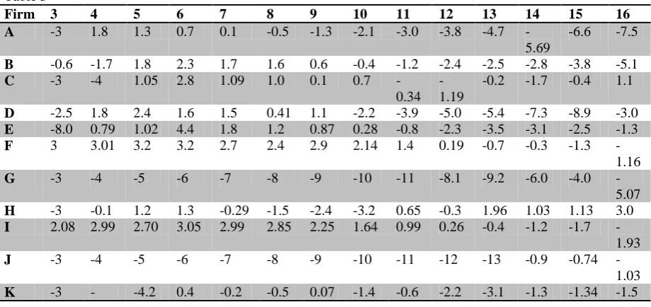
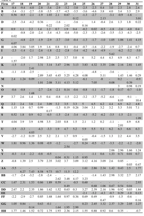
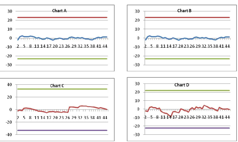
It computed for grey model to see if this model forecasting is in control or not. The result are shown in tables 3,4 and 5.

As it is seen, the forecast is completely in control and the plots of tracking signals visually display this.

Table 3

Firm 3 4 5 6 7 8 9 10 11 12 13 14 15 16

A -3 1.8 1.3 0.7 0.1 -0.5 -1.3 -2.1 -3.0 -3.8 -4.7 -5.69

-6.6 -7.5

B -0.6 -1.7 1.8 2.3 1.7 1.6 0.6 -0.4 -1.2 -2.4 -2.5 -2.8 -3.8 -5.1 C -3 -4 1.05 2.8 1.09 1.0 0.1 0.7

-0.34 -1.19

-0.2 -1.7 -0.4 1.1

D -2.5 1.8 2.4 1.6 1.5 0.41 1.1 -2.2 -3.9 -5.0 -5.4 -7.3 -8.9 -3.0 E -8.0 0.79 1.02 4.4 1.8 1.2 0.87 0.28 -0.8 -2.3 -3.5 -3.1 -2.5 -1.3 F 3 3.01 3.2 3.2 2.7 2.4 2.9 2.14 1.4 0.19 -0.7 -0.3 -1.3

-1.16

G -3 -4 -5 -6 -7 -8 -9 -10 -11 -8.1 -9.2 -6.0 -4.0

-5.07 H -3 -0.1 1.2 1.3 -0.29 -1.5 -2.4 -3.2 0.65 -0.3 1.96 1.03 1.13 3.0 I 2.08 2.99 2.70 3.05 2.99 2.85 2.25 1.64 0.99 0.26 -0.4 -1.2 -1.7

-1.93

J -3 -4 -5 -6 -7 -8 -9 -10 -11 -12 -13 -0.9 -0.74

3.21

L 1.7 2.8 2.8 2.5 2.0 1.6 1.8 2.8 2.5 2.08 1.3 0.78 0.3 -0.5

M 3 4 3.2 2.8 4.1 3.9 3.8 3.0 3.4 3.3 2.8 3.0 1.4 3.7

N

O -3 -4 -5 -6 -5.3 -6.3 -7.3 0.6 0.1 -0.4 -1.1

P -0.9 3.4 3.1 2.3 1.4 3.1 4.3 4.9 5.1 4.8 3.8 2.9 2.1 1.7 Q -3 -2.9 -0.3 1.6 0.002 2.8 1.5 2.7 2.7 1.3 1.3 -0.1 2.1 2.6 R -3 -4 -5 -6 -5.6 -5.5 -5.8 -6.8 -8.0 -8.5

-9.75

-10 -7.0 0.1

S -3 2.1 3.3 2.8 2.6 2.0 2.3 3.3 2.5 1.6 0.7

-0.08

-0.9 0.7

T -3 -0.4 -0.5 0.2 1.1 0.3 0.6 1.9 1.4 -0.18

-0.9 -1.3 -0.05 1.1

U -3 -2.5 -3.7 -4.8 -5.9 -6.9 -8 -6.1 -7.2 -8.3 -9.3 -10.2

-11.2 -3.5

V -3 -4 -5 -6 -7 -8 -9 -5.0 -6.1 -7.3 -8.4 -9.0 -10 -1.5 W -3 1.5 2.11 1.58 2.03 2.52 3.17 4.76 6.0 4.96 3.8 4.5 3.25 2.22 X

Y 1.4 2.41 1.61 1.48 1.59 2.12 1.88 1.06 0.04 0.69 -0.28

-1.3 -0.84 0.29

Z -0.8 -0.2 0.44 -1.5 -2.51 -4.15 -5.44 -6.67 -7.75 -8.91 -10.1 -3.82

-2.75 -1.21

AA -3 -4 -5 -6 -7 -8 -9 -10 -3.7

-4.31 -5.02

-5.6 -5.87 -6.99 BB 3 2.45 1.86 1.44 0.72

-0.01

1.0 0.58 -0.28

-0.79

-1.7 -0.55

-1.09 -1.4

CC -0.9 -0.5 -0.74

1.44 1.16 -0.75 -2.22 -3.46 -4.23 -4.81 -5.44 -6.69

-6.72 -1.48 DD -1.3 -2.7

-3.93 -4.48

-3.22 -4.32 -4.42 -5.54 -6.84 -7.81 -7.86 -9.08

2.13 2.94

EE

FF 0.71 0.52 0.19 0.54 0.36 -0.5 -1.21

-0.38

-0.19

1.35 1.63 1.83 1.52 1.54

GG 0.04 -0.07

-0.05

-0.86

-2.94 -4.3 0.42 -1.0 -1.4 -2.72

-4.2 1.18 -0.04 1.5

HH -3 -4 -5 -6 -4.2 -5.0 -6.0 1.97 2.97 2.45 2.0 2.28 2.54 2.34 II -2.3 -3.6

-1.87 -2.91

-4.24 -5.6 -2.4 -2.6 -3.4 -4.6 -5.9 -6.6 0.25 -1.2

JJ -3 -4 -1.68

-0.26 KK -3 -0.7 4.22 5.27 6.18 7.19 7.48 8.33 8.61 9.42 10.0 10.5 11.1 11.9

LL -3 -4 -5 -6 -5.11

-5.94 -6.79

-7.9 -8.0 -3.4 -3.99

-0.28

-1.73 -2.77

MM -3 -4 0.78

-0.52

1.85 2.2 1.66 1.87 1.01 0.4 -0.27

-0.62

4.3 3.66

NN -3 -4 -5 -6 -4.53

-5.22 -1.91

2.62 2.4 1.83 1.6 1.4 1.81 0.85

OO -0.5 0.54 1.59 2.8 1.37 0.89 0.37 -0.22

-1.32

-2.35

-3.7 -4.74

-5.45 -6.13 PP -0.2 2.23 3.11 2.45 2.73 0.86

-0.33 -1.42

-2.3 -3.58

-5.08

-5.98

-2.89 -1.26 QQ -3 1.47

-0.36 -1.93

-1.84 -3.04 -4.33 -1.34 -1.83 -2.12 -0.19

-1.4 0.005 -0.63 RR 0.16 2.44 1.99 1.85 2.98 1.56 0.26 1.47 1.11 0.08

-0.57 -1.66

0.37 0.57

SS 0.1 -1.22

-2.39

-3.5 -4.58 -5.64

Table 4

Firm 17 18 19 20 21 22 23 24 25 26 27 28 29 30 31

A -8.4 -9.4 -4.0 -2.8 -3.6 -2.9 -3.2 -3.0 -2.5 -2.3 0.4 3.0 2.3 2.8 2.6 B -3.4 -3.1 -2.7 -3.8 -3.5 -3.7 -4.5 -3.5 -3.6 -4.6 3.8 4.0 3.4 3.3 2.9 C 0.56 -0.5 -2.1 -1.9 1.03 2.1 0.67

-0.12

-1.3 -2.7 -2.13

-3.1 -0.9 -1.6 -3.01 D -2.5 -3.4 -4.2 0.36

-0.22

-1.6 -2.02

-3.6 -0.16

1.4 -0.4 2.6 1.3 1.8 0.22

E 0.9 1.1 2.2 1.4 1.2 0.7 1.9 0.4 -0.2 0.02 -0.5 -1.8 -2.6 -4.0 0.4

F

-0.02

-0.8 -2.0 -2.4 -3.4 -4.3 -4.6 -5.0 -2.3 -3.3 -2.6 -3.5 -3.3 -4.3 -2.5

G

-6.07

-4.8 -2.5 -1.9 -2.9 -3.7 -3.0 -0.4 -1.3 -1.7 -1.0 1.05 1.06 1.41 4.15

H 4.06 3.84 3.05 1.9 1.6 0.8 0.1 -0.4 -0.7 -1.6 -2.2 -1.9 -2.7 -2.4 0.7 I -2.3 -1.4 -2.1 -2.6 -1.8 -2.2 -2.8 -3.4 -4.2 -4.4 -4.9

-5.62

-6.2 -3.2 -3.0

J

-1.57

-2.0 1.7 2.98 2.5 2.5 3.7 5.0 6 5.2 4.4 4.3 4.9 4.3 4.7

K -1.5 -1.5 -2.41

3.31 3.14 3.47 2.96 3.13 3.83 4.32 3.35 2.06 2.16 2.81 1.45

L -1.1 -1.8 -2.5 -2.89 -3.65 -4.45 -5.25 -4.28 -4.08

-4.8 -5.11

-3.6 -1.43

-1.46

-0.29 M 2.4 1.24 0.09

-1.01 -2.08 -3.11 -4.13 -5.12

-6.1 -7.05

-8 -0.08

0.2 -0.39

-0.9

N 3 0.98 0.19

O -0.6 -0.8 -1.68

-2.7 -2.6 -2.1 0.14 -0.6 -0.8 -1.1 -1.7 -1.8 0.17 -0.7 -1.0

P 3.7 2.6 1.4 1.5 0.4 -0.8 -1.5 -2.2 -3.2 -3.7 -5.2 -6.6 -8.05

-9.1 -10.4 Q 2.2 2.4 3.8 2.4 3.09 3.2 3.5 3.3 5 6.5 6.2 4.4 6.9 6.2 4.8 R 1.15 1.8 0.7 0.99

-0.17

-1.3 0.19 0.26 3.04 3.1 3.2 3.2 5.3 5.01 7.1

S 0.52 1.8 0.9 0.2 -0.5 -1.5 -2.4 -3.4 -4.3 -5.2 -6.2 -3.5 -1.5 -2.1 -1.09 T 4.04 3.9 3.9 4.98 3.5 2.03 0.8 1.5 2.1 1.2 0.2 -1.1

-2.01

4.9 6.8

U -3.5 -3.3 -4.03

-4.3 -3.3 1.9 4.7 5.2 5.9 5.5 5.1 6.2 6.3 6.6 6.3

V -2.7 -1.2 0.19 2.5 3.2 2.1 1.7 0.9 -0.05

-0.4 -1.5 1.3 2.2 4.4 3.5

W 1.81 0.96 1.36 0.08 -0.9 -1.2 -2.54

-2.7 0.24 -0.5 -1.7 -3.3 -2.2 -1.2 -2.0

X 2.06 2.96 1.66 1.24

Y -0.3 -1.4 -2.2 -0.8 -0.5 -0.04 -0.31 -1.15 -0.95

-1.1 0.6 1.33 0.71 0.01 0.7

Z -0.8 1.39 2.5 3.79 2.35 3.02 3.7 3.09 3.12 4.16 3.09 2.6 0.85 -0.03

-0.47 AA -5.5

-6.27 -7.43 -8.58 -9.73 -10.7 -11.5 -12.2

1.61 2.86 2.34 1.42 0.43 2.5 1.77

BB -1.7 -2.4 -3.2 -2.8 -2.4 -2.62 -3.48 -4.17 -3.23

-1.4 1.43 2.98 3.32 2.7 2.17

CC 1.67 2.31 1.53 0.86 1.89 0.59 -0.49

-0.5 0.60 -0.68 -1.06 -0.67 -0.54 -0.04 2.93

DD 2.67 2.2 2.35 1.86 1.62 1.52 0.63 0.3 3.27 2.39 2.16 1.96 0.92 0.03 1.84

EE -2.1 -3.2 -4.3 -0.7 0.29 -1.0 0.13

FF -2.2 -2.9 -2.7 0.85 1.68 1.64 0.97 0.36 0.69 0.49 -0.47

-0.9 -1.5 -0.6 -0.16 GG 1.05 0.84

-0.14

0.63 -0.1 -1.64

-1.95

-2.99

0.23 2.45 3.32 2.37 3.29 2.05 2.27

0.08 II 1.11 0.13 -1.0 1.13 1.43 0.55

-0.25 -1.25

-1.05

-1.8 1.74 4.1 3.34 2.34 4.14

JJ -0.8 -2.4 -3.9 -4.6 -5.7 -2.82

-0.6 -1.13

-2.41

-0.02

2.55 3.43 4.41 3.57 2.45

KK 13.0 12.5 13.4 13.6 14.3 14.0 13.9 14.6 12.7 10.8 11.4 9.35 9.02 6.83 7.24 LL -3.2 -4.2 0.13 1.51 -0.1

-1.48 -3.04 -3.96 -5.09

-6.4 -7.9 -9.2 -2.2 -1.4 3.61

MM 2.3 2.64 2.18 0.97 0.69 -0.46 -1.14 -1.56 -3.08

-3.3 -2.3 -3.9 -4.9 -2.9 -1.4

NN -0.2 -0.9 -1.7 -2.3 -2.9 -3.77 -3.83 -2.68 -3.31

-2.2 1.33 1.8 0.65 1.66 1.93

OO

-5.37 -6.35 -6.07 -7.04 -2.81 -2.29 -3.59 -2.84

1.81 2.29 3.68 3.72 5.01 6.74 6.06

PP

-1.12 -0.03

-1.5 0.69 1.5 0.43 -0.64 -1.12 -2.22 -3.09

0.19 1.27 2.33 2.27 1.51

QQ -1.9 1.89 3.08 3.07 2.11 1.07 1.33 1.02 1.56 1.05 -0.41

1.28 1.57 2.49 1.17

RR

-0.07

1.15 -0.13 -1.38 -2.03 -3.32 -3.97 -5.22

-5.8 -6.25 -3.85 -3.07 -1.68 -2.84 -1.41 SS 1.39 1.32 1.03 0.34

-0.65 -1.55 -2.55 -3.25 -3.69 -2.34 -2.13 -2.94 -3.85 -4.15 -0.54 Table5

Firm 32 33 34 35 36 37 38 39 40 41 42 43 44 45

A 3.1 3.9 3.9 4.3 4.0 3.1 3.0 2.9 2.0 1.6 0.9 0.85 0.5 -0.4 B 5.6 5.9 5.3 5.2 4.4 4.5 4.0 3.7 2.9 1.9 2.6 1.9 1.0 0.3 C -3.5 -2.6 -2.2 -3.6 -2.8 1.7 2.3 4.91 5.1 3.90 2.8 1.5 0.9 -0.07 D 4.55 3.5 2.16 1.07 1.25 0.20

-1.02 -1.92

1.9 0.69 0.05 0.07 0.26 -0.2

E 2.11 0.97 0.81 0.15 -0.7 -1.8 2.47 1.63 1.83 2.15 2.1 1.3 0.3 0.3

F

-1.31

-0.71 -0.6 1.4 1.46 1.51 0.76 0.82 -0.22 1.88 1.53 1.19 0.29 0.04

G 4.3 3.5 3.09 2. 1.73 1.51 2.4 1.48 0.75 -0.01

-1.1 -0.7 -0.09 -1.5

H 1.2 0.5 0.27 0.30 0.61 -0.49

-1.04

-1.7 -2.2 1.27 0.29 1.09 0.07 0.4

I -1.6 -0.8 -1.3 -0.6 0.5 0.12 0.01 1.3 2.8 4.0 3.9 3.6 3.3 3.3 J 3.92 4.04 3.58 3.6 3.81 4.1 3.87 3.73 3.06 2.6 2.01 1.65 1 0.22 K 0.97 0.5 0.48 1.05 1.5 0.73 0.23 0.02 -0.1 1.23 2.4 2.57 1.02 0.61

L

-0.29

-0.51 -0.87

-0.7 -1.3 -1.3 -1.84

-2.16

1.11 0.67 1.04 2.67 2.27 2.98

M -1.5 -1.29 -1.8 -2.2 -2.4 -2.8 -3.36

-3.88

-1.14 -1.16

-0.48 -1.07 -1.2 2.07

N 0.97 -0.28 -0.36

-1.31

-2.02

-1.2 0.31 -0.08

-0.73 -1.89

2.07 1.99 1.56 0.87

O 2.49 2.14 1.02 1.12 2.7 2.4 3.9 4.4 4.16 3.29 2.4 2.38 1.26 -0.1

P

-4.53

-5.2 -3.1 -2.5 -3.3 1.6 3.5 3.02 3.48 3.11 2.7 1.98 0.91 -0.11

Q 6.7 5.4 5.07 4.9 6.17 6.7 7.01 6.9 7.7 8.5 10.1 10.5 8.59 8.98 R 8.27 7.3 7.6 6.8 6.7 5.6 4.2 4.15 5.15 4.12 3.45 3.12 1.91 1.71

S

-0.92

-0.08 -0.53

-0.6 -0.97

1.13 0.53 0.54 0.7 0.92 0.98 1 0.78 0.14

T 6.02 5.49 4.57 3.47 2.68 1.95 1.29 0.61 2.05 2.33 2.28 1.96 1.08 -0.02 U 5.58 4.9 4.76 3.9 3.78 3.68 2.8 1.8 2.05 1.46 1.61 0.56 -0.48 0.12 V 3.5 3.2 1.9 1.8 1.4 0.3 -0.8 -1.1 0.25 -0.2 2.4 1.3 1.8 0.37

W

-2.06

-3.2 -3.62

X 0.54 -0.86 -2.03

-2.9 -3.3 -1.86

-0.28

0.02 2.59 2.89 2.84 1.93 1.46 0.841

Y

-0.10

0.6 -0.49 -0.90 -0.99 -1.57 -2.05 -0.52

0.31 1.0 0.19 1.29 1.07 1.08

Z 1.74 1.42 1.46 4.63 4.16 2.11 0.75 -1.26

-0.57 -1.3 -1.26 2.11 3.74 1.6

AA 2.2 1.194 0.12 0.08 -0.01 -0.07 -0.21 -0.99

-2.05 -0.47

-1.0 -0.66 -1.53 -2.37

BB 2.15 2.89 2.29 1.79 1.74 1.64 1.13 1.32 1.28 2.6 1.87 1.71 1.2 0.91 CC 2.4 2.97 2.72 3.01 2.6 2.2 1.03 2.26 1.37 0.82 2.57 1.15 1.42 0.14 DD 1.2 0.25

-0.69

-1.6 2.89 2.85 2.28 1.81 1.35 1.07 2.06 1.93 0.89 0.15

EE 0.94 0.5 -0.12

-0.7 -0.52

-0.07

0.95 -0.23

3.89 2.47 1.31 1.88 0.96 0.15

FF 0.7 0.52 0.19 0.54 0.36 -0.5 -1.21

-0.38

-0.19 1.3 1.63 1.83 1.52 1.54

GG 0.94 2.21 0.58 1.02 0.94 -0.51

1.82 1.11 1.33 3.16 4.4 5.5 4.86 2.52

HH

-0.81

-0.37 1.23 3.53 4.75 5.19 5.51 4.69 4.09 3.22 2.57 2.66 1.73 0.82

II 3.44 2.88 2.03 1.8 1.15 0.71 0.33 -0.36

-0.82 1.1 1.4 0.99 0.67 0.13

JJ 2.52 1.75 1.26 0.53 0.25 1.7 1.84 2.54 1.78 1.71 1.92 1.33 0.46 0.32 KK 9.39 11.28 9.1 7.79 8.78 6.77 3.94 4.18 5.31 22.1 20.45 18.34 16.81 14.94 LL 4.73 3.24 1.76 0.21

-1.27 -2.22 -3.09 -4.09

-4.26 -5.5 -6.22 -5.2 -3.02 -3.97

MM -1.0 -1.7 -0.48

-1.64

-2.9 -0.62

0.93 0.79 1.17 -0.43

2.14 2.07 0.4 -0.27

NN 2.21 1.32 0.32 2.96 2.99 1.78 1.2 0.5 0.001 0.66 0.48 0.2 -0.31 -0.22 OO 5.1 4.42 3.93 3.31 2.68 2.38 2.08 1.03 0.35 0.20 0.35 0.87 0.45 0.24 PP 1.07 1.22 1.36 0.36 0.63 2.43 2.83 2.08 2.44 3.33 2.93 2.58 1.55 0.41 QQ 1.15 0.04

-0.79 -1.34

-2.62

-1.0 2.27 1.74 0.71 -0.26

2.61 1.44 1.29 0.29

RR 0.38 2.54 3.0 2.96 2.99 2.71 2.59 3.97 3.61 2.66 1.76 1.79 0.99 0.2 SS 0.48 0.07 2.7 2.91 1.83 0.85 0.1

-0.69

-1.2 0.38 -0.73 -1.53 -0.94 -0.57

3.4. T-test exam

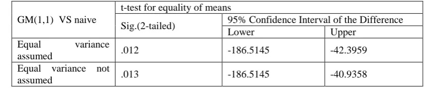
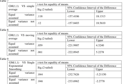
The two sample t-test simply tests whether or not two independent populations have different mean values on some measure. Here the mean square of errors in grey model as a measure of comparison are compared with mean square of errors in time series forecasting models. As it is seen in tables 7 and 8 the null hypothesis has been accepted(“p-value” is bigger than .05), which can be concluded, grey model has the same mean square of errors with moving average and simple average forecasting models. But in comparison of grey model with naive and single exponential smoothing forecasting models(table6 and9), the null hypothesis rejected, which mean they have a different mean square of errors. As it seen in table 7 and 11 for both models, lower and upper interval difference have the negative value which can be concluded that mean square of errors in grey model are less than mean square of errors in naive and single exponential smoothing model. So with more emphasis ,we can accept that grey model has the better ability in forecasting in comparison of naive and single exponential smoothing models.

Table 6

GM(1,1) VS naive

t-test for equality of means

Sig.(2-tailed) 95% Confidence Interval of the Difference

Lower Upper

Equal variance

assumed .012 -186.5145 -42.3959

Equal variance not

Table 7

GM(1,1) VS simple average

t-test for equality of means

Sig.(2-tailed) 95% Confidence Interval of the Difference

Lower Upper

Equal variance

assumed .118 -157.4106 18.1313

Equal variance not

assumed .12 -157.8403 18.5610

Table 8

GM(1,1) VS moving average

t-test for equality of means

Sig.(2-tailed) 95% Confidence Interval of the Difference

Lower Upper

Equal variance

assumed .059 -221.9907 4.3240

Equal variance not

assumed .061 -222.8945 5.2278

Table 9

GM(1,1) VS Single Exponential

Smoothing

t-test for equality of means

Sig.(2-tailed) 95% Confidence Interval of the Difference

Lower Upper

Equal variance

assumed .044 -232.7626 -3.21150

Equal variance not

assumed .046 -233.6962 -2.2778

3.5. Forecast next year’s portfolio’s rate of return

After the predictive ability of grey model ,in comparison of time series based forecasting methods, was proved ,we forecast portfolio’s rate of return for 12 months later.(march 2010 to march 2011).The result is shown in table 10.

Firm 2010 2011

Apr May Jun Jul Aug Sep Oct Nov Dec Jan Feb Mar

BB 5.23 5.14 5.05 4.95 4.87 4.78 4.69 4.61 4.52 4.44 4.36 4.28 CC 9.40 9.38 9.36 9.35 9.33 9.31 9.29 9.28 9.26 9.24 9.22 9.21 DD 8.79 8.77 8.75 8.72 8.70 8.68 8.66 8.63 8.61 8.59 8.57 8.54 EE 6.69 6.67 6.64 6.62 6.59 6.56 6.54 6.51 6.48 6.46 6.43 6.41 FF 3.97 3.90 3.82 3.75 3.67 3.60 3.53 3.47 3.40 3.33 3.27 3.21 GG 9.68 9.91 10.14 10.37 10.61 10.85 11.10 11.36 11.62 11.89 12.17 12.45 HH 3.37 3.31 3.26 3.20 3.15 3.09 3.04 2.99 2.94 2.89 2.84 2.79 II 7.32 7.30 7.27 7.25 7.23 7.21 7.19 7.17 7.14 7.12 7.10 7.08 JJ 9.24 9.18 9.11 9.05 8.99 8.93 8.87 8.81 8.76 8.70 8.64 8.58 KK 27.72 29.39 31.15 33.01 34.99 37.09 39.31 41.67 44.17 46.81 49.62 52.59 LL 11.67 11.92 12.18 12.45 12.72 13.00 13.28 13.58 13.87 14.17 14.48 14.80 MM 6.76 6.84 6.92 7.00 7.08 7.16 7.25 7.33 7.42 7.51 7.60 7.69 NN 10.15 10.21 10.27 10.32 10.38 10.44 10.49 10.55 10.61 10.67 10.73 10.79 OO 8.76 8.71 8.67 8.62 8.58 8.53 8.49 8.44 8.40 8.35 8.31 8.26 PP 11.55 11.48 11.41 11.34 11.28 11.21 11.14 11.08 11.01 10.95 10.88 10.82 QQ 5.75 5.72 5.69 5.65 5.62 5.59 5.55 5.52 5.49 5.46 5.42 5.39 RR 11.33 11.28 11.23 11.19 11.14 11.09 11.05 11.00 10.95 10.91 10.86 10.82 SS 13.43 13.59 13.75 13.92 14.08 14.25 14.42 14.59 14.76 14.94 15.11 15.29 Table 10

4. CONCLUSIONS

We proposed grey model as an accurate forecasting method for predicting stock market. We choose stock market of Tehran as a data base and gathered information of portfolio’s rate of return of 50 companies in stock market which was announced as the best companies last year. At first we computed squares sum of errors with different value of α, which could differ from .1 to .9, to insure that grey model with α=.5 is the most appropriate model in forecasting. The results showed just 5 companies from 45 have the less value of errors with α=.5, in comparison of model with the other value of α. Then we computed mean squares sum of errors with different type of time series based forecasting methods, which is here, Naïve method, Simple Average method , Moving Average method, single Exponential Smoothing method. The comparison of grey model’s errors and the errors of timed series forecasting method confirmed the predictive ability of grey model. by tacking signals we confirmed that grey model forecasting was in control. At the last, portfolio’s rate of return computed for next 12 periods.

Plots:

REFERENCES

1. Atsalakis, George&Kimon P.Valavanis (2009). ”Forecasting stock market short-term trends using a neuro-fuzzy based methodology”. Expert Systemwith Applications, VOL.36, PP.10696-10707.

2. Chen,Tai-Liang;Cheng,Ching-Hsue&Hia-Jong Teoh(2008) ”High-order fuzzy time series based on multi-period adaptation model for forecasting stock markets” Physica A,VOL.387,PP.876-888.

3. Ebrahimpour, Reza; Nikoo, Hossein; Masoudnia, Saeed;Yousefi, Mohammad Reza &Ghaemi,MohammadSajjad(2010) “Mixture of MLP-experts for trend forecasting of time series:A case study of the Tehran stock market” International Journal of Forecasting, ??

4. Hassan,Md.Rafiul (2009) “A combination of hidden Markov model and fuzzy model for stock market forecasting” Neurocommputing,VOL.72,PP.3439-3446.

5. Henri Nyberg (2011). “Forecasting the direction of US stock market with dynamic binary probit models” International Journal of Forecasting, VOL.27,PP.561-578.

6. Hsieh,Tsung-Jung;Hsiao,Hsiao-Fen& Wei-Chang Yeh (2011).” Forecasting stock markets using wavelet transform and recurrent neural networks: An integrated system based on artificial bee colony algorithm” Applied soft computing, VOL.11, PP.2510-2525.

7. Hsu, Yen-Tseng; Liu, Ming-Chung; Yeh, Jerome &Hui-Fen Hung (2009)."forecasting the turning time of stock market based on markov-fouriergreymodel" department of computer science and informationengineering,VOL.36,PP.8597-8603.

8. Hsu,Li-Chang(2009)."forecasting the output of integrated circuit industry using genetic algorithm based multivariable grey optimization models" department of inance,VOL.36,PP.7898-7903.

9. Huang,Kuangyu&Chuen-Jiuan Jane(2009)"A hybrid model for stock market forecasting and portfolio selection based on ARX ,grey system and RS theories"Expert systems with application,VOL.36,PP.5387-5392.

10. Li,Guo-Dong;Yamaguchi,daisuke&Masatake Nagai(2007)."A grey-based decision-making approach to the supplier selection problem"Mathematical and computer modeling,VOL.46,PP.573-581.

11. Lin, Yong-Huang;Lee,Pin-Chan& Ta-peng Chang (2009)."Adaptive and high-precision grey forcastingmodel"department of constructionengineering,VOL.36,PP 9658-9662.

12. Liu, Sifeng&Yi Lin(2006).Grey information,springer-verlag London limited. 13. Mynatt,jenai(2009).encyclopedia of management,GALE.

14. T.Leung,Mark;daouk,Hazem& An-Sing Chen(2000) “Forecasting stock market indices: a comparison of classification and level estimation models” International Journal of Forecasting, VOL.16,PP.173-190. 15. Yu Huang,Kuang(2009) “Application of VPRS model with enhanced threshold parameter selection

mechanism to automatic stock market forecasting and portfolio selection” Expert System with Application, VOL.36,PP.11652-11661.

16. Yeh,Chi-Yuan;Huang,Chi-Wei&Shie-Jue Lee(2011) “A multiple-kernel support vector regression approach for stock market price forecasting” Expert System withApplication, VOL.38, pp.2177-2186.