Three-dimensional simulation of the Ring effect in observations of scattered sun light using Monte Carlo radiative transfer models

Atmos. Meas. Tech., 2, 113–124, 2009 www.atmos-meas-tech.net/2/113/2009/

© Author(s) 2009. This work is distributed under the Creative Commons Attribution 3.0 License.

Atmospheric

Measurement

Techniques

Three-dimensional simulation of the Ring effect in observations of

scattered sun light using Monte Carlo radiative transfer models

T. Wagner1, S. Beirle1, and T. Deutschmann2

1_{Max-Planck-Institute for Chemistry, Mainz, Germany}

2_{Institut f¨ur Umweltphysik, University of Heidelberg, Heidelberg, Germany}

Received: 16 December 2008 – Published in Atmos. Meas. Tech. Discuss.: 14 January 2009 Revised: 9 April 2009 – Accepted: 14 April 2009 – Published: 22 April 2009

Abstract. We present a new technique for the quantitative

simulation of the “Ring effect” for scattered light observa-tions from various platforms and under different atmospheric situations. The method is based on radiative transfer calcu-lations at only one wavelengthλ0 in the wavelength range under consideration, and is thus computationally fast. The strength of the Ring effect is calculated from statistical prop-erties of the photon paths for a given situation, which makes Monte Carlo radiative transfer models in particular appro-priate. We quantify the Ring effect by the so called rota-tional Raman scattering probability, the probability that an observed photon has undergone a rotational Raman scatter-ing event. The Raman scatterscatter-ing probability is independent from the spectral resolution of the instrument and can easily be converted into various definitions used to characterise the strength of the Ring effect. We compare the results of our method to the results of previous studies and in general good quantitative agreement is found. In addition to the simulation of the Ring effect, we developed a detailed retrieval strategy for the analysis of the Ring effect based on DOAS retrievals, which allows the precise determination of the strength of the Ring effect for a specific wavelength while using the spectral information within a larger spectral interval around the se-lected wavelength. Using our technique, we simulated syn-thetic satellite observation of an atmospheric scenario with a finite cloud illuminated from different sun positions. The strength of the Ring effect depends systematically on the measurement geometry, and is strongest if the satellite points to the side of the cloud which lies in the shadow of the sun.

Correspondence to: T. Wagner

([email protected])

1 Introduction

The Ring effect describes the so-called “filling-in” of solar Fraunhofer lines in the spectra of scattered light compared to direct sun light observations. It was first observed by Shefov (1959) and Grainger and Ring (1962). Today, it is commonly agreed that rotational Raman scattering (RRS) on atmospheric molecules is the dominant source for the Ring effect (Brinkmann, 1968; Kattawar et al., 1981; Solomon et al., 1987; Bussemer 1993). Note that also the signal of vibra-tional Raman scattering in ocean water has been observed in satellite spectra (Vasilkov et al., 2002; Vountas et al., 2003), with typically much smaller amplitude than that of atmo-spheric RRS. In many atmoatmo-spheric remote sensing applica-tions that make use of scattered solar radiation (e.g. from ground based, airborne or satellite based observations), the accurate correction of the Ring effect is an important pre-requisite for the precise retrieval of atmospheric trace gas absorptions (Noxon et al., 1979; McKenzie and Johnston, 1982; Solomon et al., 1987; Chance et al., 1991; Platt and Stutz, 2008; Chance and Spurr 1997; Vountas et al., 1998; Sioris and Evans 2000; Aben et al., 2001; de Beek et al., 2001; Wagner et al., 2002, 2004). Usually, for that purpose a so called Ring spectrum is calculated and included in the spectral fitting process; it can be obtained from observations using polarisation filters or can be computed from measured solar spectra (Solomon et al., 1987; Bussemer 1993; Voun-tas, 1998; de Beek et al., 2001).

Apart from the complicating effects of RRS on atmo-spheric trace gas retrievals, observations of the Ring effect can also be used to investigate details of atmospheric ra-diative transfer. The filling-in of Fraunhofer lines depends in particular on the presence and properties of clouds and aerosols. Thus from the measured strength of the Ring ef-fect information on these quantities can be obtained (Park et al., 1986; Joiner et al., 1995, 2002, 2004, 2006; Joiner and Bhartia 1995; de Beek et al., 2001; Wagner et al., 2004;

van Deelen et al., 2007). However, this information has so far been only partly utilised because especially the numeri-cal modelling of the Ring effect is difficult and usually very time-consuming.

Here we present a new method for the precise and fast modelling of the Ring effect for various observation geome-tries and atmospheric scenarios. It is based on the full spher-ical Monte-Carlo radiative transfer models TRACY-2 and its successor McArtim (Deutschmann, 2008; Deutschmann and Wagner, 2008; Wagner et al., 2007). In contrast to existing methods for the simulation of the Ring effect (e.g. Joiner et al., 1995; Joiner and Bhartia, 1995; Vountas et al., 1998; de Beek et al., 2001; van Deelen et al., 2005; Spurr et al., 2008), our method is not based on the full simulation of the mea-sured spectra. Instead, from a simulated ensemble of photons that contribute to a given measurement, the average proba-bility of photons that have undergone RRS is calculated. For such an evaluation of the scattering statistics, Monte Carlo models are particularly well suited. Our model simulations are performed at only a single wavelength within the selected wavelength range. The method is based on the idea that the strength of the Ring effect is directly proportional to the per-centage of all simulated photons that have undergone a RRS event (e.g. Joiner et al., 1995; Wagner et al., 2004; Lang-ford et al., 2007). This fraction can be easily obtained from Monte Carlo simulations by forming the ratio of the rotation-ally Raman scattered photons to all photons. Monte Carlo radiative transfer models are especially well suited for the simulation of 3-dimensional gradients of atmospheric prop-erties like e.g. clouds.

Our paper is structured as follows: first in Sect. 2 the the-oretical basis of the new method is outlined. In Sect. 3 the details of the implementation in our Monte-Carlo radiative transfer models is described. In Sect. 4 the results of our method are compared to previous studies. Finally, the po-tential of the Monte-Carlo simulation of the Ring effect is demonstrated for the case of a finite cloud. In two appen-dices we discuss (a) the uncertainties of the technique and (b) describe how the strength of the Ring effect can be anal-ysed from DOAS measurements in an universal way.

2 Theoretical basis of the new method

2.1 Formulation of the atmospheric radiative transfer

using transmission terms

If Monte-Carlo models are applied for the simulation of the Ring effect, it is convenient to describe the atmospheric ra-diative transfer using atmospheric transmission terms. Here we use the term transmission in an broader sense than for ob-servations with a well defined geometrical absorption path: the atmospheric transmission includes not only the extinc-tion along the light path (due to scattering and absorpextinc-tion),

but depends also on the distribution and properties of scatter-ing processes and reflection on the earth’s surface.

For observations of scattered sun light in the earth’s atmo-sphere, the signal measured at a selected wavelengthλ can be described as follows:

R(λ)=I (λ)· 1

π ·Tatm(λ) (1)

Here R(λ) is the spectral radiance (e.g. in units of W/m2/sr/nm) measured by a specified detector (located e.g. on the ground or in space). I(λ)is the solar irradiance (e.g. in units of W/m2/nm) and Tatm(λ)is the atmospheric “transmission”. For observations of reflected light,Tatm(λ) is also referred to as normalised radiance.

In the atmosphere, not only elastic processes occur, but also inelastic processes like Raman scattering, which change the wavelength of the scattered photon. To account for such processes, the measured radiance can be split into three terms, one term including photons having undergone only elastic processes and two additional terms including photons, which have undergone at least one inelastic scattering (or re-flection) process.

Rtot(λ)=Rel(λ)+Rinel,in(λ)−Rinel,out(λ) (2) Rel(λ)describes the radiance for the (hypothetical) case that all photons were only elastically scattered, Rinel,in(λ) de-scribes the contribution which was inelastically scattered from the incident sun light (from various wavelengths) to the measured signal at wavelength λ,Rinel,out(λ)describes the inelastically scattered photons which originated from the sun at wavelengthλ, and reached the detector at a wavelength different fromλ.

We are primarily interested in the atmospheric Ring effect caused by rotational Raman scattering (RRS) on air molecules. Thus, as contributions to Rinel,in(λ) and Rinel,out(λ)we will in the following consider only photons, which have undergone RRS events along their path through the atmosphere (besides possible other elastic processes). Note that this concept can be extended to the description of other inelastic processes like e.g. vibrational Raman scatter-ing in the oceans.

2.2 Calculation of the Ring spectrum

In the application of the DOAS method it is common practise to correct for the spectral structures caused by the Ring effect by including a Ring spectrum in the spectral retrieval process. Usually the Ring spectrum is defined as (e.g. Solomon et al., 1987; Bussemer, 1993; Vountas, 1998, de Beek et al., 2001): f (λ)= Rinel,in(λ)−Rinel,out(λ)

Rel(λ)

(3) A Ring spectrum can e.g. be derived from polarised mea-surements under clear sky conditions (Solomon et al., 1987).

T. Wagner et al.: Three-dimensional Ring effect simulations 115 Sometimes the termRinel,out(λ)is not considered for the

cal-culation of the Ring spectrum leading to a different amplitude of the Ring spectrum but similar spectral shape (e.g. Busse-mer, 1993). For more details on the definition of Ring spec-tra and the underlying assumptions please refer to (Vountas, 1998).

In the following we apply 2 approximations in order to transform the above equation into a more suitable form. The errors caused by these approximations are typically rather small (below 1%); they are discussed and quantified in the first appendix of this paper.

The first approximation is that for the terms including ro-tational Raman scattered light, we consider only light paths which have experienced exactly one RRS event. For most sit-uations, the probability for multiple Raman scattering and the associated error are rather small (see section first appendix). The second approximation is that the dependence of the transmission on λ is neglected over the relevant spectral range of about λ±2 nm. Over this wavelength range the probability for scattering events and the surface reflectivity typically varies only slightly (see first appendix).

With these assumptions the terms including RRS in Eq. (2) can be approximated by the following expressions:

Rinel,in(λ)≈Tinel(λ)· λ+1λ

Z

λ−1λ I (λ0)

π ·F λ, λ

0

dλ0 (4)

Rinel,out(λ)≈Tinel(λ)· I (λ)

π λ+1λ

Z

λ−1λ

F λ0, λdλ0 (5)

HereTinel(λ)describes the transmission for photon paths of single Raman-scattered photons under the assumption that their wavelength wouldn’t have changed after the RRS event. F λ0, λ

describes the probability that a photon with the ini-tial wavelengthλis scattered to a new wavelengthλ0after a RRS event. F λ0, λ

is derived from the Raman scattering cross sectionσRaman(λ0,λ)by normalisation:

F λ0, λ= σRaman λ

0_{, λ}

R

σRaman(λ0, λ) dλ0

=>

λ+1λ

Z

λ−1λ

F λ0, λdλ0=1 (6)

Note that the integrals have to be evaluated only over a small wavelength interval aroundλ, for whichF λ0, λ6=0.

Now, the Ring spectrum (Eq. 3) can be described as:

f (λ)=

Tinel(λ)· λ+1λ

R λ−1λ

I (λ0₎

π ·F λ, λ

0 ·dλ0_−T

inel(λ)·I (λ)π λ+1λ

R λ−1λ

F λ0_{, λ} ·dλ0

I (λ) π ·Tel(λ)

=Tinel(λ) Tel(λ)

· λ+1λ

R

λ−1λ

I (λ0)·F λ, λ0·dλ0−I (λ)

I (λ) (7)

Figures

0% 2% 4% 6% 8%

300 350 400 450 500 550 600

Wavelength [nm] PRaman

from radiative transfer model for satellite geometry

ratio of scattering cross sections

Fig. 1 Wavelength dependence of the RRS probability (PRaman(λ)) for satellite observations for clear skies (magenta line). The satellite results are obtained using our radiative transfer model assuming a surface albedo of 5% and a solar zenith angle of 20°. For comparison, also the ratio of the cross sections for rotational Raman and Rayleigh scattering are shown (blue line) (values taken from Kattawar et al. [1981]).

22

Fig. 1. Wavelength dependence of the RRS probability (PRaman(λ))

for satellite observations for clear skies (magenta line). The satellite results are obtained using our radiative transfer model assuming a

surface albedo of 5% and a solar zenith angle of 20◦. For

compar-ison, also the ratio of the cross sections for rotational Raman and Rayleigh scattering are shown (blue line) (values taken from Kat-tawar et al., 1981).

The Ring spectrum is now expressed by two terms: the first term describes the probability of a photon to have under-gone a RRS process; it varies smoothly with wavelength and we refer to it as rotational Raman scattering probability PRaman(λ)(see Fig. 1):

PRaman(λ)=

Tinel(λ) Tel(λ)

(8) In Fig. 1 PRaman(λ) is shown for satellite nadir observa-tions under clear sky condiobserva-tions. For comparison, also the ratio of the total rotational Raman cross section and the Rayleigh cross section is shown. The wavelength depen-dence ofPRaman(λ)is stronger for the satellite observation because of two effects: at small wavelengths the RRS proba-bility is enhanced because of the higher probaproba-bility for mul-tiple scattering. At large wavelengths the RRS probability is decreased because of the higher probability of surface re-flection (increasing the number of photons which have only undergone elastic processes).

The second term of Eq. (7) contains the high frequency spectral features of the Ring spectrum and we refer to this term as normalised Ring spectrumfnorm(λ)(see Figs. 2, 3):

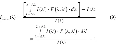
fnorm(λ)=

"

λ+1λ

R

λ−1λ

I (λ0)·F λ, λ0_·

dλ0

#

−I (λ)

I (λ) (9)

= λ+1λ

R

λ−1λ

I (λ0)·F λ, λ0·dλ0

I (λ) −1

fnorm(λ) can be derived from a solar spectrum (e.g. mea-sured by the same instrument as used for the analysis) and

320 340 360 380 400 Wavelength [nm]

In

te

n

s

it

y [a

rb.

u

n

it

s]

-1 1 3

320 340 360 380 400

320 340 360 380 400

Wavelength [nm]

Intensit

y

[arb

.

u

n

its]

-1 1 3

320 340 360 380 400

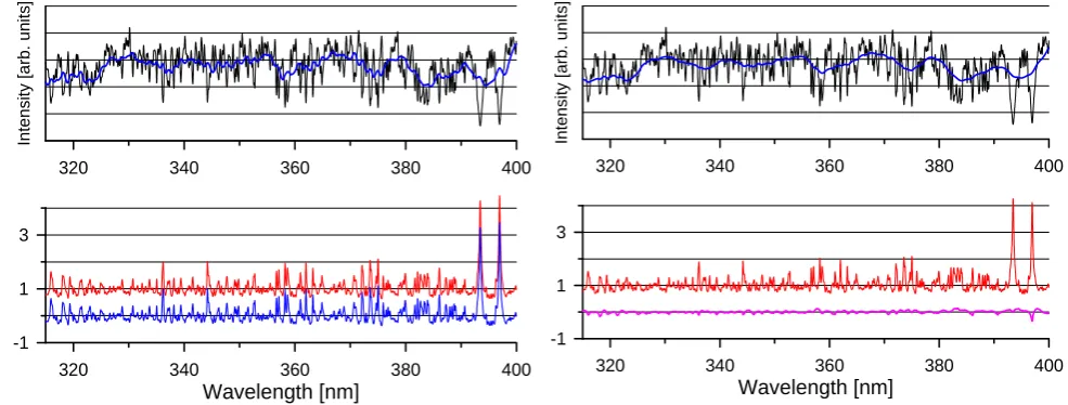
Fig. 2 Left: calculation of the normalised Ring spectrum according to Eq. 9. In the upper

panel a solar spectrum (black) for the GOME spectral resolution of ~0.17nm is shown. Also

shown (blue line) is the Raman spectrum (

), see Eq. 7). The red

spectrum in the lower panel shows the ratio of both spectra. The blue spectrum is the

normalised Ring spectrum according to Eq. 9. Right: similar as left, but including two RRS

events in the calculation. The magenta curve at the bottom right is the difference between the

Ring spectra for one and two RRS events.

(

)

∫

+

∆ −

⋅

⋅

=

λ λ

λ

λ

λ

λ

'

)

,

'

'

(

F

d

I

I

23

Fig. 2. Left: calculation of the normalised Ring spectrum according to Eq. (9). In the upper panel a solar spectrum (black) for the GOME

spectral resolution of∼0.17 nm is shown. Also shown (blue line) is the Raman spectrum (IRaman=

λ+1λ R λ−1λ

I (λ0)·F λ, λ0

·dλ0), see Eq. 7).

The red spectrum in the lower panel shows the ratio of both spectra. The blue spectrum is the normalised Ring spectrum according to Eq. (9). Right: similar as left, but including two RRS events in the calculation. The magenta curve at the bottom right is the difference between the Ring spectra for one and two RRS events.

the Raman cross section taken from literature (e.g. Kattawar et al., 1981). With these definitions, Eq. (7) can be written as:

f (λ)=PRaman(λ)·fnorm(λ) (10)

A split into a high-frequent and low-frequent terms was also discussed in Joiner et al. (1995) and Joiner and Vasilkov (2006). It is interesting to note that PRaman(λ) for a given wavelength can be derived using radiative trans-fer simulations restricted to only this wavelength (with the second approximation mentioned above). Moreover, since PRaman(λ) itself varies only weakly with wavelength (see Fig. 1), the Ring effect for wavelength ranges in the order of a few nanometers can be well approximated by calculating PRaman(λ)for only a single wavelengthλ0within the selected wavelength interval. Then Eq. (10) becomes:

f (λ)≈PRaman(λ0)·fnorm(λ) (11)

This largely reduces the computational effort for the calcu-lation of the Ring spectrum. As shown in the appendix, the wavelength dependence ofPRaman(λ)can be well accounted for when the results of the radiative transfer calculations are compared to measurements of the Ring effect.

It might be interesting to note that the content of Eq. (11) has been implicitly used for several years in typical DOAS analyses, where a Ring spectrum (containing the high-frequency part of the filling-in) is included in the spectral retrieval procedure (Solomon et al., 1987). In such cases the strength of the filling-in is quantified by the determined fit

coefficient for the Ring spectrum. Iffnorm(λ)is used in the DOAS analysis, the fit coefficient directly yields the Raman scattering probabilityPRaman(λ).

While in principle any measurement of the solar spectrum (with a spectral resolution better than that of the measure-ments to be analysed) can be used for the calculation of fnorm(λ)(see also Joiner et al., 1995), the use of a spectrum measured by the same instrument as used for the analysis (with limited spectral resolution) has an important advantage. Using such a spectrum as input ensures that the derived nor-malised Ring spectrum (and thus also the Ring spectrum it-self) has the appropriate spectral resolution and spectral sam-pling to be used in the DOAS analysis of the atmospheric spectra measured with the same instrument. Usually, Ring spectra calculated from such spectra lead to smaller residu-als in the DOAS retrieval (see residu-also Liu et al., 2005). The mathematical justification for the use of a measured spec-trum (with reduced spectral resolution) instead of a highly resolved solar spectrum is that both convolutions (the convo-lution caused by the RRS and the convoconvo-lution caused by the band-pass of the instruments) can be exchanged.

If instead a highly resolved solar spectrum is used for I(λ),

both the denominator and the numerator in Eq. (9) first have to be convoluted with the instrument function of the own spectrometer before the ratio is calculated.

The new formulation of the Ring effect has several advan-tages:

(a) The motivation and important consequence of this for-mulation is that from radiative transfer models including

T. Wagner et al.: Three-dimensional Ring effect simulations 117 RRS, this term can be directly calculated. The

determina-tion ofPRaman(λ)becomes especially easy for Monte-Carlo radiative transfer models (see Sect. 3). One important (be-cause time saving) advantage of this formulation is that for the determination ofPRaman(λ)radiative transfer simulations can be restricted to a single wavelengthλ0within the wave-length interval of interest.

(b) Our formalism allows a direct comparability between the results from radiative transfer modelling and from the DOAS analysis: if the normalised Ring spectrum is included in a DOAS analysis, the derived fit coefficient directly yields the RRS probabilityPRaman(λ), which can be directly com-pared to the results from radiative transfer modelling (note that the derived fit coefficient forfnorm(λ)does not depend on whether the term –I(λ)is included in the calculation of fnorm(λ) in Eq. (9) or not, because it only adds a constant (unity) tofnorm(λ)).

(c) The description of the strength of the Ring effect us-ing the RRS probabilityPRaman(λ)provides an universal for-mulation, which can be easily transferred to other existing definitions of the “filling-in” (see Sect. 2.3). Probably more important, it becomes independent on the spectral resolution of the instrument.

2.3 Relation of the new method to other definitions of

the strength of the Ring effect

The strength of the Ring effect has been quantified in differ-ent studies using differdiffer-ent definitions. In the study of Joiner et al. (1995) a so called filling-in factor is defined, which describes the relative change of the measured radiance at a wavelength (e.g. in the center of a Fraunhofer line) caused by RRS compared to a case without RRS. A similar defi-nition is used by de Beek et al. (2001), but they determine the so called differential filling-in as difference between the line center and the line shoulders, which is typically slightly larger than the filling-in factor used by Joiner et al. (1995). de Beek et al. (2001) refer to their definition as Ring differential optical depth (Ring DOD). A more complex definition for the filling-in is used by Langford et al. (2007). They define the fractional filling-in, which describes the relative change of the depth of a Fraunhofer line due to RRS. Common to all these definitions is that the derived filling-in depends on the spectral resolution of the instrument. This in particular com-plicates the direct comparison of observational results from instruments with different spectral resolutions.

In contrast, the formulation of the strength of the Ring ef-fect given in this study (the RRS probability,PRaman(λ), as defined in Eq. 8) is independent on the spectral resolution. In addition it can be easily converted into the correspond-ing values accordcorrespond-ing to the various definitions of the fillcorrespond-ing- filling-in, if the spectral resolution of the respective instrument is known. The general procedure for this conversion is indi-cated in Fig. 3 and is briefly outlined below:

360 370 380 390 400

Wavelength [nm]

360 370 380 390 400

Wavelength [nm]

P

from

RTM

360 370 380 390 400

360 370 380 390 400 360 370 380 390 400

Strength of

Ring effect

for various

defintions

R

′

f

f

R

′

I

C

C

C

*

P

+

Comparison

(eq. 9)

(eq. 10)

(eq. 12) (eq. 8)

360 370 380 390 400

Wavelength [nm]

360 370 380 390 400

Wavelength [nm]

P

from

RTM

360 370 380 390 400

360 370 380 390 400 360 370 380 390 400

Strength of

Ring effect

for various

defintions

R

′

f

f

R

′

I

C

C

C

*

P

+

Comparison

(eq. 9)

(eq. 10)

(eq. 12) (eq. 8)

Fig. 3 Scheme for the determination of the relation of the Raman scattering probability

PRaman(λ) and the strength of the Ring effect according to different definitions (for details see

text). CIF and CRam indicate convolution with the instrument slit function and the normalised

Raman cross sections, respectively.

24

Fig. 3. Scheme for the determination of the relation of the Raman

scattering probabilityPRaman(λ)and the strength of the Ring effect

according to different definitions (for details see text). CI F and

CRamindicate convolution with the instrument slit function and the

normalised Raman cross sections, respectively.

(a) First a “measured” spectrum is approximated accord-ing to the spectral resolution of the instrument, and the spec-ified viewing geometry and the atmospheric properties. This spectrum is calculated as follows:

R_tot0 (λ)=R_el0 (λ)·[1+f (λ)] (12) Rel0(λ)is calculated from a high resolution solar spectrum by convolution with the slit function of the instrument. The Ring spectrum f(λ)is calculated according to Eqs. (9) and (10) by substituting I(λ)byRel0(λ)and usingPRaman(λ)obtained from the radiative transfer simulation.

Note thatRel0(λ)andRtot0(λ)are different from the quan-tities used in Eq. (2) and following, sinceRel0(λ)does not contain the effects of atmospheric elastic scattering, reflec-tion on the surface and absorpreflec-tion, which would cause mod-ifications of the amplitude. For simplicity here the true elas-tically transmitted radiance is instead approximated by the convoluted solar spectrum. However, for the quantification of the Ring effect according to the above mentioned defi-nitions only relative quantities are important, which do not depend on the absolute value of the amplitude.

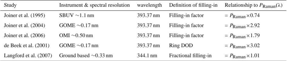
Table 1. Relationship between the Raman scattering probabilityPRaman(λ)and other definitions of the filling-in.

Study Instrument & spectral resolution wavelength Definition of filling-in Relationship to PRaman(λ)

Joiner et al. (1995) SBUV∼1.1 nm 393.37 nm Filling-in factor =PRaman×0.74

Joiner et al. (2004) GOME∼0.17 nm 393.37 nm Filling-in factor =PRaman×2.92

Joiner et al. (2006) OMI∼0.50 nm 393.37 nm Filling-in factor =PRaman×1.79

de Beek et al. (2001) GOME∼0.17 nm 393.37 nm Ring DOD =PRaman×3.02

Langford et al. (2007) Ground based∼0.33 nm 344.1 nm Fractional filling-in =PRaman×1.01

(b) In the second step, the various definitions for the quan-tification of the Ring effect (see above) can be applied to the calculated spectra. For the above mentioned examples the following procedures have to be applied:

The filling-in factor (Joiner et al., 1995) at a given wave-length is directly represented by the Ring spectrum f(λ)at that wavelength.

The differential filling-in (de Beek et al., 2001) is also de-termined from the Ring spectrum f(λ). For the chosen Fraun-hofer line the values of f(λ)at the line center and the line shoulders have to be taken into consideration.

The fractional filling-in (as defined e.g. in Langford et al., 2007) is derived from the ratio of the optical depths of the selected Fraunhofer line inRtot0(λ)andRel0(λ), respectively. Note that in case, also other quantification schemes for the Ring effect can be applied to the spectra calculated in the first step.

(c) The comparison of the determined strength of the Ring effect in step (b) and the Raman scattering probabil-ityPRaman(λ)used for the calculation of the spectra in step (a) then yields the relationship between our model results and other definitions.

For the three definitions discussed above, a linear relation-ship with the Raman scattering probability is found. The spe-cific values of the proportionality factor are summarised in Table 1.

3 Determination of the rotational Raman scattering

probabilityPRamanfrom Monte-Carlo radiative

trans-fer models including Raman scattering

The rotational Raman scattering probabilityPRaman(λ)can be derived from atmospheric radiative transfer simulations, which include RRS. Since the simulations have to be per-formed for only one wavelength (within the wavelength inter-val of interest), the calculations can be performed with rather limited computational effort. While in principle,PRaman(λ) can be determined from any radiative transfer model, Monte Carlo models are in particular suited for that purpose, be-cause they allow to quantify the relative amount of photons which have undergone RRS in a very direct and simple way

by forming the ratio of the number of rotational Raman scat-tered photons to all photons. We use the full spherical Monte-Carlo atmospheric radiative transfer models TRACY-2 and its successor McArtim (Deutschmann, 2008; Deutschmann and Wagner, 2008; Wagner et al., 2007). Currently, 3-dimensional effects (see Sect. 5) are only implemented in TRACY-2, while McARTIM is optimised for effective and quick computing in 1-D geometry. All results shown in this study for horizontal homogenous cases are based on McAR-TIM; the 3-dimensional modelling results shown in Sect. 5 were determined with TRACY-2. We compared the results of both models for horizontal homogenous cases and no sig-nificant deviations were found.

The models allow the simulation of ensembles of indi-vidual photon trajectories for a given atmospheric situation. From these trajectories the average frequency of the mod-elled photons for certain interactions with atmospheric con-stituents or with the Earth’s surface are determined. The scat-tering events are modelled individually, according to their respective scattering cross sections and phase functions. In-teraction with the Earth’s surface is treated as a Lambertian reflection. In addition to elastic processes (the reflection at the surface, Rayleigh scattering at molecules, scattering on aerosol and cloud particles), also RRS events are modelled. However, in our model, RRS events are formally treated as elastic processes. But the respective scattering cross sections (integrated over the wavelength range which is relevant for RRS) and phase functions of RRS are used. The effect of leaving the wavelength unchanged is small (<1%, see dis-cussion of the second approximation in the appendix).

From the output of the Monte Carlo simulations we deter-mine the fraction of all observed photons, which have under-gone a RRS event. This fraction represents the RRS prob-abilityPRaman(λ)as defined in Eq. (8). Another important advantage of a Monte Carlo radiative transfer model is that 3-dimensional gradients can be easily implemented. Thus, in particular the effects of finite clouds on the Ring effect can be studied (see Sect. 5). The computational speed depends both on the complexity of the modelled scenario and on the required precision. To achieve an precision of 10% for the simulation of a satellite observation for a cloud-free scenario

T. Wagner et al.: Three-dimensional Ring effect simulations 119

Joiner et al., 2004 / 2006

Ring effect as function of cloud top pressure

This study

0 2 4 6 8 10 12 14

100 200 300 400 500 600 700 800 900 1000

Cloud top pressure [mb]

Filling in [

%

]

0% 2% 4% 6% 8% 10% 12% 14%

100 200 300 400 500 600 700 800 900 1000 Cloud top pressure [mb]

Filling in

SZA_0° SZA_30° SZA_45° SZA_60° SZA_70° SZA_81° SZA_88°

Ring effect as function of surface albedo for clear sky

0 2 4 6 8 10 12 14

0.03 0.23 0.43 0.63 0.83 Reflectivity

F

illin

g

in

[

%

]

0% 2% 4% 6% 8% 10% 12% 14%

0.03 0.23 0.43 0.63 0.83 Reflectivity

Filling in

SZA_0° SZA_30° SZA_45° SZA_60° SZA_70° SZA_77° SZA_84° SZA_88°

Fig. 4 Comparison of the strength of the Ring effect using the model settings according to Joiner et al. [2004] but for the properties of the OMI instrument (Joiner et al. [2006]). Clouds are treated as Lambertian surfaces. Most probable reason for the differences is a different treatment of the Earth’s sphericity. Results are kindly provided by Joanna Joiner.

25

Fig. 4. Comparison of the strength of the Ring effect using the model settings according to Joiner et al. (2004) but for the properties of

the OMI instrument (Joiner et al., 2006). Clouds are treated as Lambertian surfaces. Most probable reason for the differences is a different treatment of the Earth’s sphericity. Results are kindly provided by Joanna Joiner.

about 20 s are required on a state of the art PC (dual core processor, 2.4 GHz). For complex cloud scenarios like that presented in Sect. 6, the computation requires about 20 min.

4 Comparison of the results to previous studies

We compared our results to results from other studies (Joiner and Bhartia, 1995; Joiner et al., 1995, 2004, 2006; de Beek et al., 2001). For these comparisons we adapted the ex-act model properties (e.g. surface albedo, solar zenith angle (SZA), surface pressure, cloud top height) where possible. We treated clouds either as Lambertian reflectors or as ex-tended scattering layers with single scattering albedo of 1 and an asymmetry parameter of 0.8. In general good quali-tative and often also quantiquali-tative agreement was found. Two examples of this comparison are shown in Figs. 4 and 5.

For the comparison with the results from the model of Joiner et al. (2004, 2006) (Fig. 4) deviations are mostly found for large SZA. These differences are most probably related to the specific treatment of the earth’s sphericity. For the comparison with de Beek et al. (2001) (Fig. 5) deviations are mostly found for low cloud optical depth at high cloud top

de Beek et al. [2001]

Ring effect as function of cloud optical depth

This study

0% 2% 4% 6% 8% 10% 12% 14%

0 2 4 6 8 Cloud top Height [km]

Ring DOD OD 2

OD 5 OD 10 OD 20 OD 50 OD 100

0% 2% 4% 6% 8% 10% 12% 14%

0 2 4 6 8 Cloud top Height [km]

Ring DOD OD 2

OD 5 OD 10 OD 20 OD 50 OD 100

Fig. 5 Comparison of the strength of the Ring effect from de Beek et al. [2001] and calculated with the new method as function of cloud top pressure and cloud optical depth. A possible reason for the differences might be a different treatment of the optical properties of the cloud particles. The results are adopted from de Beek et al. [2001].

26

Fig. 5. Comparison of the strength of the Ring effect from de Beek

et al. (2001) and calculated with the new method as function of cloud top pressure and cloud optical depth. A possible reason for the differences might be a different treatment of the optical proper-ties of the cloud particles. The results are adopted from de Beek et al. (2001).

height. The reasons for these discrepancies are currently not clear, but might be partly related to the specific choice of the optical parameters of the cloud particles.

11°

13°

20km

10km cloud _80km

11°

13°

20km

10km cloud _80km

Fig. 6 Position of the satellite ‘footprints’, cloud, and sun for the case study.

27

Fig. 6. Position of the satellite “footprints”, cloud, and sun for the

case study.

Also for the comparison with the results of Joiner and Bhartia (1995) and Joiner et al. (1995) (not shown here) over-all good agreement was found.

5 Effects of 3-dimensional clouds

Monte-Carlo radiative transfer models allow a rather sim-ple treatment of 3-dimensional effects like e.g. the Earth’s sphericity or three-dimensional gradients of atmospheric trace gases, clouds or aerosols. Also complex surface to-pography can be included. In this section we show a case study demonstrating the potential effects of 3-dimensional cloud structures on the Ring effect and the normalised radi-ance (Tatm(λ)in Eq. 1). We chose a finite cloud (horizontal extension: 20×80 km2, vertical extension: 10 km) which is illuminated by the sun at different solar zenith angles, alter-natively from two sides (referred to as illuminated side and shadow side, see Fig. 6). The single scattering albedo of the cloud particles is set to 1, the asymmetry parameter to 0.8, and the vertical optical depth is 10. The satellite points either to the side or the top of the cloud (see Fig. 6): for the view on the cloud side the viewing angle was∼11◦from nadir, for the view on cloud top it was∼13◦_{; the satellite altitude was}

400 km. The surface albedo was assumed to be 5% and the atmosphere to be free of aerosols.

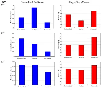
The results are shown in Fig. 7. Both, the normalised ra-diance and the strength of the Ring effect depend system-atically on the measurement geometry (viewing angle and SZA).

For low SZA (20◦_{) the highest radiance is observed from}

the cloud top. Note that the results for the cloud top are av-erages for simulations with relative azimuth angle of 0◦ _or

180◦; the results for both cases are, however, very similar. The radiance received from the sides of the cloud are smaller than from the top, with the lowest values from the shadow side. The opposite dependence is found for the Ring ef-fect indicating that for the observations with lowest radiance the relative importance of molecular scattering (and thus also RRS) is highest.

For SZA of 70◦_{the highest radiance is observed from the}

illuminated side, since the solar photons hit the cloud side at a steeper angle than the top. The smallest radiance is found from the shadow side. Again, the strongest Ring effect is found for the observation with the smallest radiance indicat-ing the increased importance of molecular scatterindicat-ing. Inter-estingly, the Ring effect for observations from the top and the illuminated side are similar. The relatively small values for the cloud top observation is probably caused by the shielding effect of the cloud.

For large SZA of (87◦) the differences for the different viewing directions become smaller indicating that an increas-ing fraction of the solar photons is scattered by molecules before they reach the cloud. Again, the Ring effect is largest for the observation pointing to the shadow side.

Our results show that including 3-D effects can be impor-tant for the proper interpretation of satellite observations of the Ring effect and the observed radiance. More research is needed to investigate these effects in sufficient detail, espe-cially their dependence on the size of the satellite footprint.

6 Conclusions

We presented a new technique for the quantitative simula-tion of the Ring effect for scattered light observasimula-tions from various platforms. The method is based on radiative transfer calculations at only one wavelength within the wavelength range of interest and is thus computationally fast. It makes use of several simplifications, but the associate errors are typ-ically below 1%. In principle the method can be applied for all radiative transfer models which include the effects of RRS. However, since it is based on statistical properties, it is particularly well suited for Monte Carlo radiative trans-fer models. We implemented the new method in our Monte Carlo radiative transfer models TRACY-2 and McARTIM. Both models are full spherical models; TRACY-2 also allows to simulate 3-dimensional fields of clouds, aerosols, trace gases or other properties like the surface topography.

Our new method describes the Ring effect by an universal quantity, the so called RRS probabilityPRaman(λ), which is independent from the spectral resolution of the instrument. It can, however, be easily converted to match different defini-tions of the strength of the Ring effect. The detailed steps for such a conversion are described. Using these conversions, the results of our method are compared to the results of pre-vious studies and in general good quantitative agreement is found.

In addition to the method for the simulation of the Ring effect, we also developed a detailed strategy for the analysis of the Ring effect based on DOAS retrievals (see appendix). It allows the precise determination of the strength of the Ring effect at a specific wavelength while using the spectral infor-mation within a larger spectral interval around the selected wavelength. The method can be applied for various viewing

T. Wagner et al.: Three-dimensional Ring effect simulations 121

SZA Normalised Radiance Ring effect (PRaman)

20°

0 0.2 0.4 0.6 0.8 1

illuminated side cloud top shadow side

Normalised radiance

0 1 2 3 4 5 6 7 8

illuminated side cloud top shadow side

Praman [%]

70°

0 0.1 0.2 0.3 0.4 0.5

illuminated side cloud top shadow side

Normal

ised radi

ance

0 1 2 3 4 5 6 7 8

illuminated side cloud top shadow side

Praman [%]

87°

0 0.01 0.02 0.03 0.04 0.05

illuminated side cloud top shadow side

Normal

ised radi

ance

0 1 2 3 4 5 6 7 8

illuminated side cloud top shadow side

Praman [%]

Fig. 7 Model results of the Ring effect (PRaman) and the normalized radiance at 370nm for the

case study described in Fig. 6.

28

Fig. 7. Model results of the Ring effect(PRaman) and the normalized radiance at 370 nm for the case study described in Fig. 6.

geometries and atmospheric situations with different contri-butions from scattering on molecules, particles as well as re-flection of the surface.

Finally we presented a case study for satellite measure-ments of a situation with a finite cloud. The strength of the Ring effect depends systematically on the measurement geometry, and is strongest if the satellite points to the side of the cloud which lies in the shadow of the sun. Since the typical satellite ground pixels of the satellite instruments used for the observation of the Ring effect is of the order of several tens of kilometres, very often partially cloudy scenes are observed in a single measurement, and the cloudy part can contain complex 3-dimensional structures. Future stud-ies should simulate and systematically investigate the depen-dence of the Ring effect for various possible 3-dimensional scenarios and compare these simulations to 1-dimensional cases. Thereby, the uncertainties of cloud retrievals based on 1-dimensional simulations of the Ring effect could be deter-mined. 3-dimensional simulations should also systematically be compared to satellite observations.

Moreover, measurements of the Ring effect should be used in synergy with measurements of the absorptions of O2and O4and the radiance at different wavelengths (de Beek et al., 2001; Wagner et al., 2004; Joiner et al., 2004) to make opti-mum use of the spectral information provided by sensors like GOME, SCIAMACHY and OMI.

Appendix A

Errors of the new method

The approximations made in Sect. 2.2 introduce errors in the simulation of the Ring effect using our new method. These errors are discussed and quantified in this appendix.

A1 Assumption 1: Neglect of multiple rotational

Ra-man scattering events

To estimate the resulting error, the probability of the mea-sured photons for multiple scattering events on molecules has to be determined. For that purpose we used our radia-tive transfer model TRACY-2 (see Sect. 3). For satellite ob-servations in the UV, the average number of molecular scat-tering events is typically between 1 and 3 per photon, de-pending mainly on wavelength, surface albedo, presence of clouds, viewing direction and solar position (for observations at longer wavelengths, especially from satellite instruments, this probability decreases and is typically <1 at 500 nm). If e.g. the average number of molecular scattering events is 2, the relative amount of multiply Raman scattered photons compared to single rotationally Raman scattered photons is typically<2%; for an average number of molecular scatter-ing of 3, it increases up to about 5%.

122 T. Wagner et al.: Three-dimensional Ring effect simulations

residual of the DOAS fit can be minimised. In addition, the fit coefficients determined for both Ring spectra in the spectral fitting procedure can even provide information on the presence of clouds or high surface albedo. In this way the advantage of an extended wavelength range can be combined with the possibility to analyse the strength of the Ring effect at a specific wavelength. For DOAS analyses using large wavelength ranges it might be interesting to include additional Ring spectra representing weak wavelength dependencies like e.g. for aerosol scattering.

320 340 360 380 400

Wavelength [nm] 0

2 4

-1 0 1

320 340 360 380 400

320 340 360 380 400

0 2 4

Original Ring spectrum

Ring spectrum for bright surfaces

Orthogonalised Ring spectrum for bright surfaces

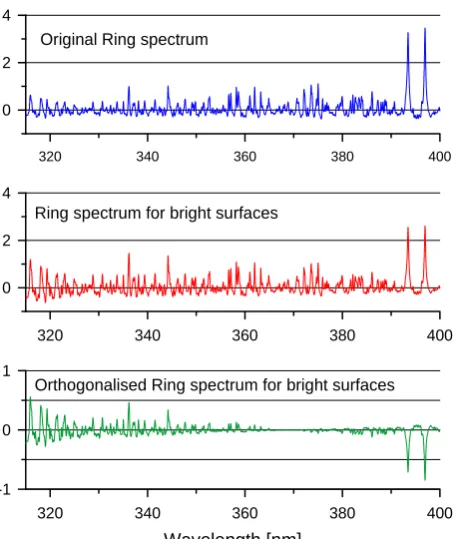
Fig. A1 Illustration of the normalisation procedure if two Ring spectra are included in the spectral DOAS analysis. The upper panel shows the original normalised Ring spectrum. In the center, a modified Ring spectrum with a different wavelength dependence of the amplitude (appropriate for bright surfaces) is shown. At the bottom this Ring spectrum is shown after normalisation with respect to the original Ring spectrum. The normalisation has to be chosen such that the amplitude of the normalised spectrum is zero at the wavelength at which the Ring effect is calculated.

32

Fig. A1. Illustration of the normalisation procedure if two Ring

spectra are included in the spectral DOAS analysis. The upper panel shows the original normalised Ring spectrum. In the center, a mod-ified Ring spectrum with a different wavelength dependence of the amplitude (appropriate for bright surfaces) is shown. At the bot-tom this Ring spectrum is shown after normalisation with respect to the original Ring spectrum. The normalisation has to be chosen such that the amplitude of the normalised spectrum is zero at the wavelength at which the Ring effect is calculated.

However, it should be noted that the resulting error of the Ring spectrum is much smaller, because also multiple rota-tional Raman scattered photons cause a filling-in of Fraun-hofer lines. The additional wavelength shift caused by the second RRS event further smoothes the Raman spectrum

F(λ)(see Fig. 2, right) and the resulting Ring spectrum for two RRS events is similar to that for one RRS event. From the small difference between both Ring spectra (<10% of the amplitude of the Ring spectrum) and the low probability for a second RRS event (<5%), we estimate the resulting total error to be far below 1%.

It might be interesting to note that in future analyses of satellite spectra with a strong filling-in, it would be an op-tion to include both Ring spectra (for single and double RRS) in the DOAS analysis. Thus it might even be pos-sible to separate the spectral features between both spectra and thus determine experimentally the probabilities of the observed photons to have undergone RRS once or twice. But this will of course be only possible for the analysis of the

strongest Fraunhofer lines. For example for the Fraunhofer lines around 390 nm, the optical depth of the difference at 397 nm might be up to 0.5%, which should be clearly de-tectable.

Finally, it might be interesting to note that within the framework of our formalism, the effect of double RRS pho-tons could be addressed in a similar way as for the single RRS photons. However, for practical applications, this ex-tension might not be necessary. Usually, the relative error caused by the multiple scattering is well below 1%.

A2 Assumption 2: Wavelength independence of the

at-mospheric transmission

For large differences (a few nm) betweenλ0andλ the de-viation of Tinel(λ) from the true value can be of the order of a few percent. Only for very high average numbers of molecular scattering the resulting error can increase to about 10%. However, this error estimate would be only valid for cases where the intensity of the solar spectrum would be completely zero at one side of wavelengthλ. For practical cases the average solar irradiance at both sides of the received wavelengthλshows much smaller variations over the rele-vant wavelength range of a few nm aroundλ. Thus the higher partial transmission forλ0<λand the lower partial transmis-sions forλ<λ0will mainly cancel each other. Even for large average numbers of molecular scattering events, the errors caused by this approximation is therefore typically<1%.

Appendix B

Determination of the rotational Raman scattering

probabilityPRamanfrom a DOAS analysis

Like various trace gas cross sections, also a Ring spectrum can be included in a DOAS fitting routine (Solomon et al., 1987; Vountas, 1998; Platt and Stutz, 2008). This proce-dure is widely used for the correction of the Ring effect while performing the spectral analysis. If a normalised Ring spectrum (as defined in Eq. 9) is included in the DOAS fit procedure, the fit coefficient directly yields the RRS proba-bilityPRaman(λ). One specific advantage of this procedure compared to the determination of the filling-in for a selected Fraunhofer line (like e.g. in Langford et al., 2007) is that in the DOAS analysis the complete information from a more extended wavelength range is used (see e.g. also Joiner et al., 2004). Thus, also the strength of the Ring effect for wave-length ranges with weak Fraunhofer lines can be well deter-mined. However, the use of an extended wavelength range has also one important disadvantage: the wavelength depen-dence of the amplitude of the Ring spectrum fits perfectly only to cases dominated by (single) Rayleigh scattering. For cases with high probability for multiple Rayleigh scattering events, or with strong contributions of surface reflection or

T. Wagner et al.: Three-dimensional Ring effect simulations 123 scattering on cloud and aerosol particles, the amplitude of

the Ring spectrum will have different wavelength dependen-cies.

Thus, if extended wavelength regions are included in the DOAS fit, the different wavelength dependencies might not well be represented by the normalised Ring spectrum (ac-cording to Eq. 9) and the fit errors can increase.

However, there is an elegant way to circumvent this prob-lem. In addition to the normalised Ring spectrum (accord-ing to Eq. 9) a second R(accord-ing spectrum can be included in the DOAS fit, for which the amplitude has a different wavelength dependence (Wagner et al., 2002; Liu et al., 2005; Langford et al., 2007). Such a second Ring spectrum can be calcu-lated from the original normalised Ring spectrum by mul-tiplication with a term which changes smoothly with wave-length. Probably a polynomial of degree 4 is best suited be-cause it can compensate for the difference between the wave-length dependencies of Rayleigh-scattering and scattering on cloud particles. Then an orthonormalisation of the second Ring spectrum with respect to the original one has to be per-formed. This orthonormalisation has to be applied in a way that at the wavelength of interest (for which the RRS proba-bility was calculated) the amplitude of the second Ring spec-trum is zero (see Fig. A1). Then the fit coefficient determined for the (original) normalised Ring spectrum directly yields the RRS probabilityPRaman(λ)at the wavelength of interest. By including two Ring spectra in the spectral analysis, the spectral residual of the DOAS fit can be minimised. In ad-dition, the fit coefficients determined for both Ring spectra in the spectral fitting procedure can even provide informa-tion on the presence of clouds or high surface albedo. In this way the advantage of an extended wavelength range can be combined with the possibility to analyse the strength of the Ring effect at a specific wavelength. For DOAS analyses using large wavelength ranges it might be interesting to in-clude additional Ring spectra representing weak wavelength dependencies like e.g. for aerosol scattering.

Acknowledgements. We like to thank Michael Grzegorski, Andreas

Richter, Joanna Joiner, Marco Vountas and R¨udiger de Beek for in-teresting discussions. Joanna Joiner, Marco Vountas and R¨udiger de Beek have kindly provided their data for comparison with our study.

The service charges for this open access publication have been covered by the Max Planck Society.

Edited by: A. Kokhanovsky

References

Aben, I., Stam, D. M., and Helderman, F.: The ring effect

in skylight polarization, Geophys. Res. Lett., 28(3), 519–522, doi:10.1029/2000GL011901, 2001.

Brinkmann, R. T.: Rotational Raman scattering in planetary atmo-spheres, Astrophys. J., 154, 1087–1093, 1968.

Bussemer, M.: Der Ring-Effekt: Ursachen und Einfluß auf die Mes-sung stratosp¨arischer Spurenstoffe, Diploma thesis, University of Heidelberg, 1993.

Chance, K. V., Burrows, J. P., and Schneider, W.: Retrieval and molecule sensitivity studies for the Global Ozone Monitoring Experiment and the SCanning Imaging Absorption spectrometer for Atmospheric CHartographY,” in: Remote Sensing of Atmo-spheric Chemistry, edited by: McElroy, J. L. and McNeal, R. J., Proc. SPIE, 1491, 151–165, 1991.

Chance, K. V. and Spurr, R. J. D.: Ring effect studies: Rayleigh scattering, including molecular parameters for rotational Raman scattering, and the Fraunhofer spectrum, Appl. Optics, 36, 5224– 5230, 1997.

Deutschmann, T.: Atmospheric radiative transfer modelling using Monte Carlo methods, Diploma thesis, University of Heidelberg, 2008.

Deutschmann, T. and Wagner, T.: TRACY-II Users manual, (http: //joseba.mpch-mainz.mpg.de/Strahlungstransport.htm), 2008. de Beek, R., Vountas, M., Rozanov, V. V., Richter, A., and Burrows,

J. P.: The Ring effect in the cloudy atmosphere, Geophys. Res. Lett., 28, 721–724, 2001.

Grainger J. F. and Ring, J.: Anomalous Fraunhofer line profiles, Nature, 193, 762, 1962.

Joiner, J., Bhartia, P. K., Cebula, R. P., Hilsenrath, E., McPeters, R. D., and Park, H.: Rotational Raman scattering – Ring effect in satellite backscatter ultraviolet measurements, Appl. Optics, 34, 4513–4525, 1995.

Joiner J. and Bhartia, P. K.: The determination of cloud pressures from rotational Raman scattering in satellite backscatter ultravi-olet measurements, J. Geophys. Res., 100, 23019–23026, 1995. Joiner, J., Vasilkov, A., Flittner, D., Buscela, E., and

Glea-son, J.: Retrieval of Cloud Pressure from Rotational

Ra-man Scattering, in: OMI Algorithm Theoretical Basis Doc-ument Volume III: Clouds, Aerosols, and Surface UV

Ir-radiance, edited by: Stammes, P., ATBD-OMI-03, Version

2.0, Aug. 2002 (http://www.knmi.nl/omi/documents/data/OMI ATBD Volume 3 V2.pdf), 31–46, 2002.

Joiner, J., Vasilkov, A. P., Flittner, D. E., Gleason, J. F., and Bhar-tia, P. K.: Retrieval of cloud pressure and oceanic chlorophyll content using Raman scattering in GOME UV measurements, J. Geophys. Res., 109, D01109, doi:10.1029/2003JD003698, 2004. Joiner, J. and Vasilkov, A. P.: First results from the OMI rotational Raman scattering cloud pressure algorithm, IEEE T. Geosci. Re-mote, 44, 5, 1272–1282, 2006.

Kattawar, G. W., Young, A. T., and Humphreys, T. J.: Inelastic-Scattering in Planetary-Atmospheres. 1. The Ring Effect, with-out Aerosols, Astrophys. J., 243(3), 1049–1057, 1981.

Langford, A. O., Schofield, R., Daniel, J. S., Portmann, R. W., Melamed, M. L., Miller, H. L., 10 Dutton, E. G., and Solomon, S.: On the variability of the Ring effect in the near ultraviolet: understanding the role of aerosols and multiple scattering, At-mos. Chem. Phys., 7, 575–586, 2007,

http://www.atmos-chem-phys.net/7/575/2007/.

Liu, X., Chance, K., Sioris, C. E., Spurr, R. J. D., Kurosu, T. P., Martin, R. V., and Newchurch, M. J.: Ozone Profile and Tropo-spheric Ozone Retrieval from Global Ozone Monitoring Exper-iment (GOME): Algorithm Description and Validation, J. Geo-phys. Res., 110(D20), D20307, doi:10.1029/2005 JD006240, 2005.

McKenzie, R. L. and Johnston, P. V.: Seasonal variations in

stratospheric NO2at 45◦S, Geophys. Res., Lett., 9, 1255, 1982.

Noxon, J. F., Whipple, Jr. E.C., and Hyde, R. S.: Stratospheric NO₂,

Observational method and behaivior at mid-latitude, J. Geophys. Res., 84, 5047, 1979.

Platt, U. and Stutz, J.: Differential Optical Absorption Spec-troscopy, Principles and Applications, Springer, Berlin, 2008. Park, H., Heath, D. F., and Mateer, C. L.: Possible application

of the Fraunhofer line filling in effect to cloud height measure-ments, Meteorological Optics, OSA Technical Digest Series, 70– 81, Opt. Soc. Am., Washington, DC, 1986.

Shefov, N. N.: Spectroscopic, photoelectric, and radar investiga-tions of the aurora and the nightglow, Izd. Akad. Nauk., 1, 1959. Sioris, C. E. and Evans, W. F. J.: Impact of rotational Raman

scat-tering in the O2A band, Geophys. Res. Lett., 27, 4085–4088,

2000.

Spurr, R. J. D., de Haan, J., van Oss, R., and Vasilkov, A. P.: Dis-crete ordinate radiative transfer in a stratified medium with first order rotational Raman scattering, J. Quant. Spectrosc. Ra., 109, 3, 404–425, 2008.

Solomon, S., Schmeltekopf, A. L., and Sanders, R. W.: On the in-terpretation of zenith sky absorption measurements, J. Geophys. Res., 92, 8311–8319, 1987.

van Deelen, R., Landgraf, J., and Aben, I.: Multiple elastic and inelastic light-scattering in the Earth’s atmosphere: A doubling-adding method to include rotational Raman scattering by air, J. Quant. Spectrosc. Ra., 95, 399–433, 2005.

van Deelen, R., Hasekamp, O. P., van Diedenhoven, B., and Landgraf, J.: Retrieval of cloud properties from near ultravi-olet, visible and near infrared satellite-based Earth reflectance spectra: a comparative study, J. Geophys. Res., 113, D12204, doi:10.1029/2007JD009129, 2007.

Vasilkov, A. P., Joiner, J., Gleason, J., and Bhartia,

P. K.: Ocean Raman scattering in satellite backscatter

UV measurements, Geophys. Res. Lett., 29(17), 1837,

doi:10.1029/2002GL0149552002.

Vountas, M.: Die Modellierung und Parametrisierung des Ring Effektes: Einfluß auf die Bestimmung von stratosph¨arischen Spurengasen, PhD-thesis, University of Bremen, (http://www. iup.physik.uni-bremen.de/diss/Vountas/ring diss/master.html), 1998.

Vountas, M., Rozanov, V. V., and Burrows, J. P.: Ring effect: Im-pact of rotational Raman scattering on radiative transfer in earth’s atmosphere, J. Quant. Spectrosc. Ra., 60(6), 943–961, 1998. Vountas, M., Richter, A., Wittrock, F., and Burrows, J. P.: Inelastic

scattering in ocean water and its impact on trace gas retrievals from satellite data, Atmos. Chem. Phys., 3, 1365–1375, 2003, http://www.atmos-chem-phys.net/3/1365/2003/.

Wagner, T., von Friedeburg, C., Wenig, M., Otten, C., and

Platt, U.: UV/vis observations of atmospheric O4absorptions

using direct moon light and zenith scattered sunlight under clear and cloudy sky conditions, J. Geophys. Res., 107, 4424, doi:10.1029/2001JD001026, 2002.

Wagner, T., Dix, B., Friedeburg, C. v., Frieß, U., Sanghavi, S., Sinreich, R., and Platt, U.: MAX-DOAS O4 measurements – a new technique to derive information on atmospheric aerosols. (I) Principles and information content, J. Geophys. Res., 109, doi:10.1029/2004JD004904, 2004.

Wagner, T., Burrows, J. P., Deutschmann, T., Dix, B., von Friede-burg, C., Frieß, U., Hendrick, F., Heue, K.-P., Irie, H., Iwabuchi, H., Kanaya, Y., Keller, J., McLinden, C. A., Oetjen, H., Palazzi, E., Petritoli, A., Platt, U., Postylyakov, O., Pukite, J., Richter, A., van Roozendael, M., Rozanov, A., Rozanov, V., Sinre-ich, R., Sanghavi, S., and Wittrock, F.: Comparison of boxair-mass-factors and radiances for Multiple-Axis Differential Opti-cal Absorption Spectroscopy (MAX-DOAS) geometries Opti- calcu-lated from different UV/visible radiative transfer models, Atmos. Chem. Phys., 7, 1809–1833, 2007,

http://www.atmos-chem-phys.net/7/1809/2007/.