3D IC PARTITIONING BY USING FAST FORCE DIRECTED SIMULATED ANNEALING ALGORITHM FOR REDUCING THROUGH-SILICON VIAS

(1)

(www.dvpublication.com) Volume 1, Issue 2, 2016

6 3D IC PARTITIONING BY USING FAST FORCE DIRECTED

SIMULATED ANNEALING ALGORITHM FOR REDUCING

THROUGH-SILICON VIAS

Dr. P. Sivaranjani* & G. Srividhya**

* Assistant Professor, Department of Electronics and Communication, Kongu Engineering College, Tamilnadu

** PG Scholar, Department of Electronics and Communication, Kongu Engineering College, Tamilnadu

Cite This Article: Dr. P. Sivaranjani & G. Srividhya, “3D IC Partitioning by Using Fast Force Directed Simulated Annealing Algorithm for Reducing Through-Silicon Vias”, International Journal of Advanced Trends in Engineering and Technology, Page Number 6-11, Volume 1, Issue 2, 2016.

Abstract:

Three dimensional(3D) integration has recently become popular due to reduction in wire length, manufacturability, power consumption and it mainly enhances the integration of Very Large Scale Integration(VLSI).As demands accelerate for increasing density, higher bandwidths and lower power, many IC manufacturing industry are looking up to 3D ICs with Through-Silicon vias.3D ICs accommodates multiple heterogeneous die and integrates great deal of functionality into small form factor, while improving performance and reducing costs. It offers new levels of efficiency, power, performance and form factor. In this paper a novel force directed simulated annealing is introduced and used for 3D partitioning. The proposed method introduces force as a new factor during the annealing process and it replaces every random move by force directed moves. The experimental results show that the proposed method speeds up the convergence, and reduces the number of Through-Silicon vias by maintaining the quality of solution when compared to conventional simulated annealing algorithm.

Key Words: 3D IC, Partitioning, Through-Silicon Vias & Force Directed Simulated Annealing 1. Introduction:

Three dimensional (3D) integration has become popular due to its smaller size and reduced interconnections. 3D IC technology definitely promises towards larger levels of integration of circuit components and miniaturization of devices in a single chip.3D IC mainly focuses on reducing the wire length and interconnect delays, and also it ensures significant improvement in the functionality and performance of large number of components by accommodating multiple heterogeneous integration of materials such as logic, memory, analog, RF and micro-electrical mechanical systems at different process nodes.3D layout can be formed by stacking the results of 2D layout. One of the biggest issues to be addressed during 3D IC integration is communication between tiers using Through-Silicon vias(TSVs).TSVs are highly expensive and they significantly occupy some chip area[].Excessive usage of TSVs leads to undesired results and have a negative impact on wire length. Since the TSVs are bulky they act as obstacles during the routing and placement process which leads to routability congestion, hence their minimization is considered as an important objective in the IC physical design stage. Many more techniques have been evolved in order to reduce the number of TSVs, one of those technique is to use effective partitioning method during the IC physical design stage. The netlist should be partitioned in such a way that the number of interconnections between the tiers should be minimized which results in reduced number of TSV usage. We propose here an algorithm that performs multi-level partitioning in order to minimize the total number of TSVs. The rest of the chapters are organized as follows. In section 2, the literature survey on 3D IC and Simulated annealing is given. In section 3 the 3D partitioning problem is given. In section 4, the proposed method is discussed in detail. In section 5 the experimental results of SA and FSA is shown and the results are compared.

2. Related Works:

(2)

7

allocation and optimization purpose that considers total wire length, thermal optimization and TSV resource sharing possibilities. The simulated annealing based on metropolis algorithm. Simulated annealing is applicable to many combinatorial optimization problem such as travelling salesman problem [9], vehicle routing, supply chain management and machine scheduling.

3. Problem Formulation:

In a three dimensional circuit, partitions are arranged on top of each other and the connection between two adjacent tier requires one TSV whereas the connection between two non-adjacent tiers requires more than one TSVs. Hence the goal of three dimensional techniques is to form the desired number of tiers in such a way that the total number of TSVs required should be minimized.

Figure 1: a) TSV usage is 8 Figure 1: b) TSV usage is 7

Figure 1: Partitions are arranged in proper order for reducing the number of TSVs. And therefore the 3D partitioning problem can be formulated as

min em ,n∈∅we m − n (1)

s.t v∈V_iarea v ≤∝× 1/k v∈Varea(V)

Where ∅ indicates set of cut nets, we indicates Weight of net e, V is the set of cells and K is the total number

of partitions, and α represents the imbalance factor. The techniques that are applied to 2D circuits are not appropriate for 3D circuits.

 In a three dimensional circuits the position of tiers has an impact on the TSVs count. In the fig.1 a) shows the partitions are placed in an order and the number of TSVs required is eight, whereas in the fig.1 b) the order of partitions are changed which results in the reduction of TSV usage to seven.  The generated partitions for two dimensional circuits are not always the favorable partitions targeting

3D partitioning even though they are placed in the best stacking order which is shown in figure 2. In figure 2 a) the nodes are assigned to the tiers and it represents the best two dimensional partitioning solution of a circuit is shown in which the number of 2D net cuts is six and the number of three dimensional net cuts is equal to eight. The alternative partitioning solution for the similar circuit is shown in the figure 2. In the figure 2 b) which shows the seven two dimensional net cuts and seven 3D net cuts. The figure 2 represents example showing that best partitions for 3D circuits differs from best partitions targeting 2D circuits.

Figure 2: a) Optimal partitioning solution targeting 2D circuit

Figure 2: b) Optimal partitioning solution targeting 3D circuit

Figure 2: An example that shows the optimal 2D partitioning solution is not always the optimal 3D partitioning solution.

4. Simulated Annealing Algorithm:

(3)

8

continued until the particles are rearranged in the ground state of the solid. Initially the random solution is generated and temperature value is set. After initializing the temperature the looping condition starts and it continues until the stopping criterion is met:

 Either the system is sufficiently cooled

 The algorithm stops when it finds an optimal solution.

Then the neighbor solution is selected by making a small change to the current solution. Then the appropriate decision has to be made whether to move to that neighbor solution. Finally the temperature is decreased and the looping is continued till the stopping criterion is satisfied.

A. Acceptance Function: The law of thermodynamics state that at temperature t, the probability of an increase in energy of magnitude ∆E is given by

P(∆E) = exp(-∆E /kt) (2)

Where, k is a constant known as Boltzmann constant. If the energy has decreased then the system moves to this state. If the energy has increased then the new state is accepted.

B. Temperature Initialization:

It is essential to select the temperature value that will initially allow for practically any moves against the current solution so that better exploration will be taken place.

Input : Initial Solution Output: Optimized Solution Simulated_annealing() begin

solution = initial solution; cost = Evaluate(solution);

Temperature = Initial temperature; while(temperature > final temperature)do Newsolution = mutate(solution)

Newcost = evaluate(newsolution) ∆cost = Newcost – cost

If(∆cost ≤ 0)then Cost = newcost; Solution = newsolution; end

Temperature = cooling rate.temperature end

return the best solution; end

Algorithm I Simulated Annealing:

One of the parameters to the algorithm is the cooling schedule. This algorithm assumes that the annealing process will continue until the temperature reaches zero or some other criterion is met. A constant number of iteration is done at each temperature, at the lower temperature it is important that a large number of iterations are done so that the local optimum can be fully explored and at higher temperatures, the number of iterations can be less.

5. Proposed Methodology:

The fast force directed simulated annealing follows the annealing process and the modification is incorporated in the already existing simulated annealing method. In the standard simulated annealing the present solution is altered by the random nearby solution whereas in the proposed method selection of new solution is based on the probability. The probability of selecting the neighbor solution depends on the data given to the system that can be modeled as molecular forces. Thus the selection of the neighbor solution based on the force rather than the randomized approach is more effective in finding an appropriate move, and this approach makes the algorithm to converge quickly and it escapes from the local optimum solution. In three dimensional partitioning problems the data is modeled as forces connected cells impose on each other [3].In the proposed method the circuit is modeled as mass-spring system where the cells and nets are same as the masses and springs.The proposed work algorithm is described below

Input: Initial Solution 𝑆Init

Output: Refined solution Generate the initial solution Initialize the temperature.

Calculate the forces on each cell and cost of each cell while T> Tmindo

while stopping criterion is not met yet do

(4)

9

costnew ← cost(sʹ)

∆cost = costnew − costcurrent

if∆cost < 0

s ← sʹ//Move updates

costcurrent ← costnew

f=forces(s) //Force updates elser ← Random 0,1

ifr < e−∆cost /T_then

s← sʹ costcurrent ← costnew

f=forces(s) //Force updates end if

end if end while T← ∝. T

end while

Algorithm II Force Directed Simulated Annealing:

A. Initialization: For the initial solution the circuit is divided into several partitions with the goal of reducing the connections between the partitions. And then the every initial partition are placed on top of each other and each partition is referred to as the layer.

B. Force Calculation: Forces are applied to the connected cells that are placed in different layer. And the forces applied to the cells pulls the connected cell close together and place those cells in the same layer or the adjacent layer in order to reduce the TSV usage. Forces need not to be applied to the cell which is located in the same layer or the adjacent layer since the TSVs required is minimum in these cases. However the cells are assigned to the tiers in order to reduce the complexity of the algorithm and the force calculation of each cell is given below

fab = Ca,b zb− za 0 ≤ a, b ≤ n(3)

Where Ca,b is the connection weight between cell a and cell b and zb and zaare the locations of the cell b and a

on the z-axes, respectively. Many of the cells does not require any force as all the cells are situated in the same layer (Z𝑖 = Z𝑗) these cells are not considered for moves.

C. Cell Selection: The cell is allowed to move only if it improves the solution ie., it should decrease the total cost or passes the probability condition otherwise the procedure is repeated again until the desired cell is selected as a candidate cell to move. Here the cost of the solution is equal to total number of TSVs required. The force simulated annealing neighbor function consists of two steps

 Selecting the cell to be moved: The cell is selected randomly and allowed to move with various probabilities based on the forces applied on them which means if f𝑖 is the force applied to each cell its

selection probability will be

𝑃𝑖 = 𝑓𝑖 𝑓𝑗 𝑗 (4)

 Assigning new location to the selected cell: The selected candidate cell is moved either to the same tier or the adjacent tier. The initial temperature can be calculated by using the Boltzmann distribution

P0= e−Ave (cost )/T0 => −𝐴𝑣𝑒(𝑐𝑜𝑠𝑡)/ln (5)

Where P0 is the initial probability of acceptance of uphill moves. The annealing schedule gives the rate

of decreasing temperature and it is given by

𝑇𝑖+1 = ∝× 𝑇𝑖 (6)

Where 𝑇𝑖+1 and 𝑇𝑖 represent the temperature at steps i+1 and I respectively. The number of iterations

should be set in such a way that the runtime should not increase and the algorithm should not get trapped in a local optima. The algorithm stops if it reaches the minimum temperature value or it reaches the maximum number of iterations.

6. Experimental Results:

Force directed simulated annealing is proposed to perform the refinement step of 3D partitioning of circuits. Here the total number of TSV required for FSA is compared with the TSVs required for SA algorithm for the ibm01 benchmark circuit and the results are tabulated below

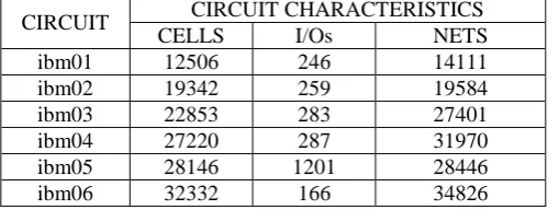
Table 1: ISPD 2004 benchmark circuits statistics includes number of cells,I/O pads, and nets.

CIRCUIT CIRCUIT CHARACTERISTICS

CELLS I/Os NETS

ibm01 12506 246 14111

ibm02 19342 259 19584

ibm03 22853 283 27401

ibm04 27220 287 31970

ibm05 28146 1201 28446

(5)

10

ibm07 45639 287 48117

ibm08 51023 286 50513

ibm09 53110 285 60902

Ibm10 68685 744 75196

Ibm11 70152 406 81454

ibm12 70439 637 77240

ibm13 83709 490 99666

ibm14 147088 517 152772

ibm15 161187 383 186608

Ibm16 182980 504 190048

Ibm17 184752 743 189581

Ibm18 210341 272 201920

Parameter Settings:

The initial temperature 𝑇𝑜is set to decide on the probability of accepting an uphill move initially and it

can be easily calculated by using Boltzmann distribution and it is given in equation (5). The different annealing schedule between 0.4 to 0.9 were tested and alpha = 0.4 is chosen as best quality time trade-off. The number of TSVs reduction with variation in alpha is shown in table II.III.IV and V And then the next parameter is number of iterations, at each temperature sufficient number of moves need to be performed and there is no defined rule on determining this number and it is generally set empirically. If this number is set too high, the runtime of algorithm increases without much change in the result and if the number is set too low the algorithm might get trapped in local optimum. Here, it is proposed to set this number proportional to temperature ie., less number of iterations for higher temperature and more number of iterations for low temperatures. The algorithm stops when the temperature reaches its minimum value (𝑇𝑚𝑖𝑛) and the algorithm terminates when the number of iterations

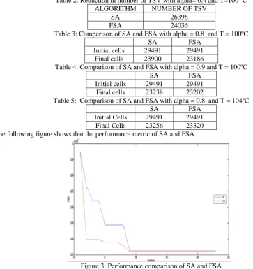
exceeds the maximum number of iteration. The following table shows the reduction in total number of TSVs used with variation in the value of alpha and temperature.

Table 2: Reduction in number of TSV with alpha= 0.4 and T=100 ºC ALGORITHM NUMBER OF TSV

SA 26396

FSA 24036

Table 3: Comparison of SA and FSA with alpha = 0.8 and T = 100ºC

SA FSA

Initial cells 29491 29491 Final cells 23900 23186

SA FSA

Initial cells 29491 29491 Final cells 23238 23202

SA FSA

Initial Cells 29491 29491 Final Cells 23256 23320 The following figure shows that the performance metric of SA and FSA.

(6)

11

7. Conclusion:

The force directed simulated annealing can be implemented as a refinement method for 3D IC partitioning aiming TSV number reduction. In this proposed work 8.76% of TSVs has been reduced in Force directed simulated annealing when compared to conventional SA, with α=0.4 and T=1000ºC, 2.98% reduction when α = 0.8 and T=100ºC and 0.15% reduction occurs when α = 0.9 and T=1000ºC. And this method can be applied in many other optimization problems. In FSA the cost function and the force calculation can be easily modified and it can be applied to various objectives.

8. Future Work:

In the future work by applying clustering techniques such as AMG (Algebraic Multi Grid) to obtain better partitioning solutions. In addition to that, Modified force directed Simulated Annealing method can also be applied for generating the desired number of tiers in a far shorter run time.

9. References:

1. Ababei C, Feng Y, Goplen B and Sapatnekar (2005) ,“Placement and routing in 3d integrated circuits”, IEEE Des.Test, Vol.22, No.6, pp.520-531

2. Byunghyunlee and Taewhankim (2014), “Algorithms for Through Silicon vias resource sharing and optimization in designing 3D stacked Integrated Circuits”, Integration of VLSI journal, Vol.47, pp.184-194.

3. Eisenmann and Johannes (1998), “Generic global placement and floor planning”, in Design Automation Conference, pp.269-274.

4. George Karypis, Rajat Aggarwal, Vipin Kumar, and Shashi Shekhar (1999), “Multilevel hyper graph partitioning: Application in VLSI domain”, IEEE transactions on very large scale Integration Systems, Vol.7, No.1, pp. 69–529.

5. He X, Dong S, and Ma Y (2010), “Signal Through the Silicon via planning and pin assignment for thermal and wire length optimization in 3D Integrated Circuits”, Integration of VLSI journal, Vol.43, No.4, pp.342-352.

6. Hong Z. Li, X, Zhou Y Cai, J. Bian and Saxena (2005) “A divide and conquer 2.5-d floor planning algorithm based on statistical wire length estimation”, in: IEEE International symposium on circuits and systems, 2005.ISCAS, Vol.6, pp. 6230-6233.

7. Hua-Sin Ye, Chi M, and Shih-Hsu Huang (2010), “A design partitioning algorithm for three dimensional Integrated Circuits”, In Computer Communication Control and Automation (3CA), Vol.36, No.98, pp. 229–232.

8. Knetchel J, Young and Lienig (2015), “Planning massive interconnects in 3D chips”, IEEE transaction on Computer Aided Design of Integrated Circuits, Vol.34, No.6, pp. 1808-1821

9. Kirkpatrick, Gelatt C and Vecchi M (1983), “Optimization by simulated annealing”, IEEE transaction on Computer Aided Design of Integrated Circuits, Vol.220, No.4598, pp.671–680.

10. Lee B, Kim T, (2014), “Algorithms for TSV resource sharing and optimization in designing 3d stacked ics”, VLSI journal, Vol.47, No.2, pp.184-194.

11. Meng Kai Hsu, Yao Wen Chang and Valeriy Balabanov (2011), “Through Silicon Vias Aware analytical placement for 3D IC Designs”, 48th ACM/EDAC/IEEE Design Automation Conference, pp.664-669.

12. Natarajan Viswanathan and Chris Chong-Nuen Chu (2005), “Efficient Analytical placement using cell shifting, Iterative local refinement and a hybrid net model”, IEEE transaction on Computer Aided Design of Integrated Circuits and Systems, Vol.24, No.5, pp.26-33.

13. Rob A. Rutenbar (1989), “Simulated Annealing Algorithmms an overview”, IEEE Circuits and Device Magazines, Vol.89, pp.755-996.

14. Sawicki S, Hentschke, and Johann (2006), “An algorithm for i/o pins partitioning targeting 3D VLSI Integrated Circuits”, In 49th IEEE International Midwest Symposium on, Vol.2, pp. 699 –703.