* Corresponding author Tel.: +601123058983 E-mail: [email protected] (A. Parnianifard) 2019 Growing Science Ltd.
doi: 10.5267/j.ijiec.2018.2.001
International Journal of Industrial Engineering Computations 10 (2019) 133–148
Contents lists available at GrowingScience
International Journal of Industrial Engineering Computations
homepage: www.GrowingScience.com/ijiecTrade-off in robustness, cost and performance by a multi-objective robust production optimization method
Amir Parnianifarda*, A.S. Azfanizama, M.K.A. Ariffina and M.I.S. Ismaila
aDepartment of Mechanical and Manufacturing Engineering, Faculty of Engineering, Universiti Putra Malaysia, 43400 UPM Serdang,
Selangor, Malaysia
C H R O N I C L E A B S T R A C T
Article history:
Received September 20 2017 Received in Revised Format December 25 2017 Accepted February 6 2018 Available online February 7 2018
Designing a production process normally is involved with some important constraints such as uncertainty, trade-off between production costs and quality, customer’s expectations and production tolerances. In this paper, a novel multi-objective robust optimization model is introduced to investigate the best levels of design variables. The primary objective is to minimize the production cost while increasing robustness and performance. The response surface methodology is utilized as a common approximation model to fit the relationship between responses and design variables in the worst-case scenario of uncertainties. The target mean ratio
is applied to ensure the quality of the process by providing the robustness for all types of quality characteristics and with a trade-off between variability and deviance from the ideal point. The Lp metric method is used to integrate all objectives in one overall function. In order to estimate target value of the quality loss by considering production tolerances, the process capability ratio ( ) is applied. At the end, a numerical chemical mixture problem is served to show the applicability of the proposed method.
© 2019 Growing Science Ltd. All rights reserved Keywords:
Robust design Loss function Uncertainty
Response surface methodology Process optimization
1. Introduction
Nowadays, most engineering design methods try to assist decision makers for optimizing the processes and achieving the highest quality with minimum costs. The process of finding the accurate design parameters is stated as an optimization. Typically, any optimization technique needs to consider design constraints. It is the engineer’s duty to choose the design parameters according to an (or some) objective
function(s) (Beyer & Sendhoff, 2007). Process optimization is one of the intensive aspects of
product development (Lukic et al., 2017). During the optimization process, we need to maximize one or more parameters, while keeping all others within their constraints. The main goal is to reach a desired performance for the process that manufactures some products, by minimizing the cost of operation in a production process, or the variability of a quality characteristics by maximizing the yield of the production process. Furthermore, due to noisy data and/or uncertainty affecting some parameters of the model, achieving robust performance plays an essential role for engineering design problems.
design aims to reduce the impact of these types of environmental factors on a product or process, and leads to greater customer satisfaction and higher operational performance. The objective of robust design is to minimize the total quality loss in products or processes. Robust design is the most powerful method available for reducing product cost, improving quality, and simultaneously reducing development time. In process robustness studies, it is desirable to minimize the influence of noises and uncertainty in the process and simultaneously determine the levels of input and control factors, by optimizing the overall responses, or in another sense, optimizing product and process, which are less sensitive to various causes of variances. By employing the information of experiments about the relationships between input control factors and output responses, robust design methods can disclose robust solutions that are less sensitive to causes of variations (Nha et al., 2013).
There are different robust optimization models proposed in the literature for design processes in engineering problems. Nevertheless, there is still a gap between theory and practice in optimization, being evident in the fact that optimization methods are still not used for many real-world problems, (Bertsimas et al., 2011; Beyer & Sendhoff, 2007). In order to increase the reliability in optimization results, uncertainty and the tradeoff between three aspects of production cost, robustness, and performance are important circumstances which need to be considered in production problems. The primary aim of this paper is to propose a new mathematical formulation of robust optimization model to find the best levels of design variables in the production process under minimum computational cost when uncertainty and the tradeoff between three aspects of production cost, robustness, and performance are attended in the problem. In addition, physical constraints to satisfy customer’s requirements and obligation to satisfy production tolerances are also considered in the model. In robust design approach, both the robustness of the objective functions (optimal results) and the constraints (feasibility) are considered, simultaneously. The proposed model is formulated by considering three different types of quality characteristics such as of Nominal The Best (NTB), Smaller The Better (STB), and Larger The Better (LTB). In order to estimate the target point applied in the expected quality loss function, a new
approach is suggested by using for all three types of characteristics. However, since we wish to
design the model with the customer’s point of view, the terms of customer tolerance ( , ) and
process capability index are used in the proposed model. In addition, the trade-off between production cost and performance with insensitivity against environmental factors is attended in designing the model, while most existing methods are just concentrated on seeking the best levels of design variables which maximizes the robustness (Gabrel et al., 2014).
The rest of the paper is organized as follows. The application of integrating robust design optimization and response surface modeling (RSM) in the literature is briefly reviewed in Section 2. In Section 3, the methodology including the required steps for constructing the proposed method is explained. This section also includes two different mathematical formulations based on process’s cost and quality loss. A numerical example (mixture problem) is served in Section 4 to illustrate the applicability of the proposed models. Finally, this paper is concluded in Section 5.
2. Literature review
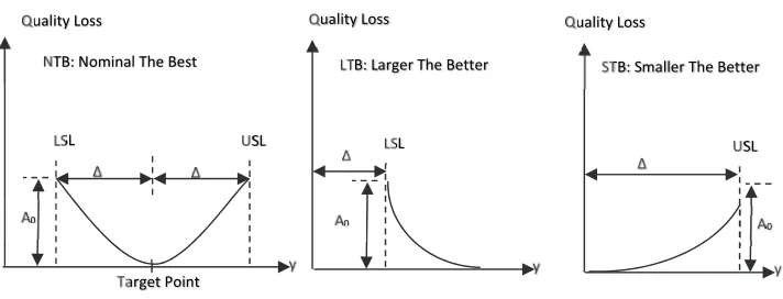
It is commonly accepted that the Taguchi’s principles are useful and very appropriate for industrial product design (Simpson et al., 2001). Taguchi also represented the concept of quality loss as an average amount of total loss that compels to society because of deviating from the ideal point and variability in responses. Moreover, this function tries to make a trade-off between the mean and variance of each type of quality characteristics (Park & Antony, 2008). Fig. 1 depicts the graphical concepts of expected loss function based on the classification of quality characteristics into three different types including NTB, LTB, and STB.
where, , , respectively are mean, variance, and target of response and is the loss coefficient.
The value of is computed by
∆ for NTB and STB and ∆ for LTB. The quality loss coefficient
can be determined on the basis of the necessary information on the losses in monetary terms caused by falling outside the customer tolerance. The coefficient plays an important role to make the expected loss function in monetary loss scales. In addition, is introduced as a cost of repair or replacement when the quality characteristic performance has the distance of ∆ from target point (Phadke, 1989). Recently, the robust optimization under uncertainty has been interested where treatments of uncertainty are described in different scenarios. A common approach in robustness studies is associated with minimizing objectives in the worst-case scenario. The min-max robustness (also called strict robustness) has been appropriately elucidated by Ben-Tal et al. (2009). The robust optimization methodology has been adopted in many applications of interest in different sciences, and it is widely used in practice for optimizing, planning, and scheduling of real processes. In Boyaci et al. (2017), a fuzzy mathematical model was developed by RSM technique and fuzzy logic to optimize drilling process optimization with multiple responses. Investigate the literature shows interesting issues in application of robust design optimization in production and manufacturing processes (e.g. Parnianifard et al., 2018).
In practice, the designer often has to deal by conflicting objectives and source of uncertainty. In the process and product optimization, a common problem is to determine optimal operating condition that balances the multiple quality characteristics of a product. There are different methods in literature for Multi-Objective Robust Optimization (MORO). The robust design approach has been combined with different methods in multi-objective optimization such as the weighted sum method (Zadeh, 1963), goal programming (Charnes & Cooper, 1977), physical programming (Messac & Ismail-Yahaya, 2002), compromise programming (Chen et al., 1999), desirability function (Chen et al., 2012; Costa et al., 2011), different metric methods (Hwang & Masud, 2012; Miettinen, 2012), and evolutionary algorithms (Deb, 2011). Computation-intensive in design problems are becoming increasingly common in production industries. Investigating all Pareto optimal solutions is computationally expensive and time-consuming,
NTB (1)
STB (2)
LTB 1 1 3 / (3)
Δ
Δ
LSL
USL
Quality Loss y Target Point 0 A NTB: Nominal The Best Δ LSL Quality Loss y 0 A LTB: Larger The Better Δ USL Quality Loss y 0 A STB: Smaller The Better
because in most cases, Pareto optimal solutions are usually exponentially large (Chinchuluun & Pardalos, 2007). In practice, difficulties arise because of different units of measurement, criteria, and levels of importance among the multiple responses or quality measurements. Moreover, some different methods have been presented which try to tackle the problem of optimizing multiple responses simultaneously, (e.g. Marler & Arora, 2004; Miettinen, 2012). Notably, preference of each method than other strongly depends on the role of decision maker and information on hand based on different purposes of the problem, (i.e. none of existing methods in the multi-objective problem can be claimed to be superior to the others in every aspect), (Miettinen, 2001).
The computation burden is often caused by expensive analysis and simulation processes in order for physical testing of data. To address such a challenge, approximation techniques (also known as metamodels or surrogate models) are often used. Approxiamtion methods have been developed in statistics, mathematics, computer science, and various engineering disciplines. These methods have been used to avoid intensive computational and numerical models, which might squander time and resources
for estimating model's parameters. If input or design variables and responses or outputs have a
relationship as , then a model can fit to approximate that relationship is , so
where represents an error of approximation (Simpson et al., 2001). Some number of common
approximation methods are polynomial regression (also called Response Surface Methodology (RSM)), Kriging, Artificial Neural Network (ANN), Radial Basis Functions (RBF), see (Simpson et al., 2001; Wang & Shan, 2007). The name of RSM might be somewhat misleading since all types of approximation methods constitute a “surface” which enables the user to predict the response at untried points. However, the common use of RSM, which is also adopted here, is to address polynomial regression models. The response surface approach facilitates understanding the system by modeling the response functions for process mean and variance, respectively. RSM is a collection of statistical and mathematical techniques useful for developing, improving, and optimizing process. The overview of the second-order response surface model is shown as:
, (4)
where , and are unknown regression coefficients and the term is the usual random error (noise) component. The accuracy of the approximation model strongly depends on designing appropriate sample points. Some experimental sampling methods are Central Composite Design (CCD), fractional factorial, Box-Behnken, alphabetical optimal, and Plackett-Burman (Myers et al., 2016).
3. Methodology
In the current work, some main assumptions and outstanding points are followed as below:
In this study, uncertainty is assumed to be fixed in the worst scenario, and under this condition we try to minimize the expected loss for each quality characteristic (response) and minimize constraint variation region. In the worst-case scenario of uncertainties, it is assumed that all variations of system performance may occur simultaneously in the worst possible combinations of design variables. Respect to the min-max approach, we try to minimize the maximum variability in the process performance due to the existence of uncertainties in their worst framework. The highest amount of process’s cost is raised due to facing process in the worst combinations of uncertainties. In addition, the variability due to fluctuating input variables is assumed as a stochastic term in the problem.
To reduce the computational complexity of the model, first we standardize all design variables
into 1, 1 , then resulted in magnitudes use in RSM proceeding for utilizing simpler regression
The fluctuating of input factors around its specific value is assumed that constructed by the existence of environmental factors (uncontrollable in practice), and it is desirable to responses do not have much variability due to its fluctuation (He et al., 2010).
3.1Nomenclature
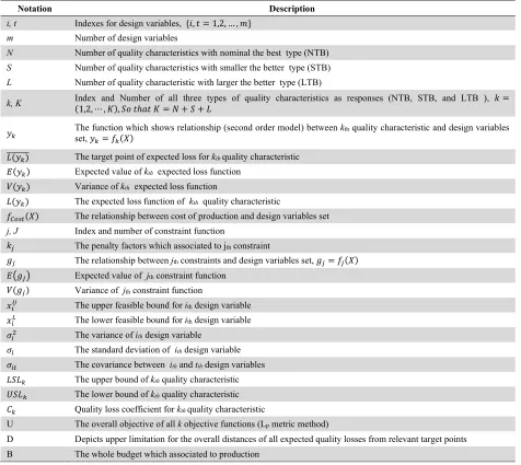
The parameters and symbols which used in the proposed method are revealed in Table 1. Table 1
The table of nomenclature
Notation Description
i, t Indexes for design variables, , 1,2, … ,
m Number of design variables
N Number of quality characteristics with nominal the best type (NTB)
S Number of quality characteristics with smaller the better type (STB)
L Number of quality characteristic with larger the better type (LTB)
k, K Index and Number of all three types of quality characteristics as responses (NTB, STB, and LTB ), 1,2, ⋯ , ,
The function which shows relationship (second order model) between kth quality characteristic and design variables set,
The target point of expected loss for kthquality characteristic
Expected value of kth expected loss function
Variance of kth expected loss function
The expected loss function of kth quality characteristic
The relationship between cost of production and design variables set
j, J Index and number of constraint function
The penalty factors which associated to jth constraint
The relationship between jth constraints and design variables set, Expected value of jth constraint function
Variance of jth constraint function
The upper feasible bound for ith design variable The lower feasible bound for ith design variable The variance of ithdesign variable
The standard deviation of ithdesign variable
The covariance between ithand tth design variables
The upper bound of kth quality characteristic
The lower bound of kth quality characteristic
Quality loss coefficient for kthquality characteristic
U The overall objective of all k objective functions (Lp metric method)
D Depicts upper limitation for the overall distances of all expected quality losses from relevant target points B The whole budget which associated to production
3.2Robustness in objective functions
considered. However, in practice for real condition of the process particularly in the production process, this kind of targeting are exaggerating (Sharma & Cudney, 2011). Also for optimizing the process, we need functions of expected quality loss that be comparable to one another in three cases of NTB, LTB, and STB. Sharma et al. (2007) proposed the target mean ratio that has a common formula for all three types and brings similarity among them. Based on their proposed target mean ratio , the expected quality loss is described as below:
1 , 1,2, … , (5)
where the is equal to ⁄ and 0 when is a large number and is a target point
for characteristic. The could be defined by the decision maker and based on the type of quality characteristic. For different values of , the expected loss represents different magnitudes for each type of NTB, LTB, and STB. This value shows the shifting of to the right or left side of the target point and can be chosen zero for STB type, a larger number more than one for LTB type and also 1 for NTB. But, it is strongly recommended that the target point and specially do not need to be a large number or infinity for LTB cases, but it just needs to be significantly greater than one, for more information see Sharma and Cudney (2011) and Sharma et al. (2007). In order to follow the customer’s satisfaction in the production process, let’s consider the target point is in the center of production tolerances, so
2 ⁄ .
3.3 Robustness in constraints set
The constraints of the production process which are classified into two groups. First the physical constraints , and second the limiting magnitude of design variables. The preferences of the designer or available resources for choosing the interest levels for design variables are some instances of physical constraints (Messac & Ismail-Yahaya, 2002). In robust design optimization, robustness in both objectives set and constraints set needs to be considered. Moreover, to study the variation of constraints, we employ the worst-case scenario approach. In the worst-case scenario of uncertainties, it is assumed that all variations of system performance may occur simultaneously in the worst possible combination of variability sources. The original constraints are modified by adding the penalty term separately to each of them as below:
. 0, 0,1,2, … , (6)
where is penalty factor of constraint which can be determined by the decision maker. This penalty factor or confidence coefficient can control the degree of robustness (Sahali et al., 2015). To achieve the feasibility of the constraint under uncertainty, a general probabilistic feasibility formulation can be
considered as 0 ∗ , 1,2, … , where ∗ is the desired probability for satisfying
constriants. If we assume is normally distributed, Φ ∗ have been suggested by Parkinson
et al. (1993) while Φ is the inverse function of the cumulative density function in a standard normal distribution.
The bounds of design variables are also modified to ensure feasibility under deviations:
, 1,2, ⋯ , (7)
3.4 Estimating of model’s parameters
1
2 . ∆ 1 2 ⋯ (8)
. . ∆ 1 2 ⋯
(9)
1
2 . ∆ 1 2 ⋯
(10)
. . ∆ 1 2 ⋯
(11)
where ∆ if and if . The expressions of the mean and variance of the relevant quality
characteristic for each objective function and also mean and variance of each physical constraint are
respectively estimated by the second-order terms of Taylor's expansion about and . Also,
the derived equations are valid for any probability density function of and . The fluctuating of the design variables around their specific values are due to the effects of environmental factors in the process.
3.5 Multi-response optimization method
In the current paper, the weighted Lp metric is used to integrate multiple objectives for all types of quality
characteristics, due to two main reasons. First, needing less information from decision maker and second compared to other multi-objective method is the ease of application in practice, (See Miettinen, 2001). Also capability ratio Cpm is used as a supplement of the Lp metric to estimate the target value of each
expected loss. The weighted Lp metric method can define the desired point and try to find an optimal
solution that is as close as possible to this point (Chinchuluun & Pardalos, 2007). This method appropriately has been applied in the robust multi-objective to find a Pareto optimal solution, (See Ardakani & Noorossana, 2008).
3.5.1 Overall function
In the current work, the Lp metric is used to measure the distance between the expected loss of each
quality characteristic and the relevant target point. Notable that all responses have the same scales due to the existence of coefficient in expected loss formulation, which make them in scale of monetary. The overall function which is utilized to integrate all responses is:
min . (12)
Here is the target point for expected loss, the quantity of shows the importance of
expected loss compared to others and can take a value between zero and one, so that ∑ 1 and
3.5.2 Estimating the target point
In current paper, the desired capability of the process is used to estimate the target magnitude of each expected loss function. The process capability was proposed by Chan et al. (1988). In this index, the numerator is the range of the tolerance interval ( – ) of the process which illustrates customer’s limitations. The denominator is a combined measure of the standard deviation and the deviation of the mean from the target value. This ratio derives the mean square deviation related to Taguchi’s loss function. The capability index for NTB is clearer than STB and NTB type. In the production process for quality characteristics with NTB type we do not need to allocate a large number or infinity for upper specification level (Sharma et al., 2007). Also for the same reason for STB types, the value of zero for the lower specification is exaggerative. So we can assume the upper and lower specification level is
times greater than for NTB types and times smaller than for STB types of quality
characteristics, while 1. The twofold more than the target point for in the case of LTB have been recommended by Sharma and Cudney (2011). So, if the middle value between upper and lower
specification assumes the ideal value for the performance of quality characteristics, then 4 is
suggested to be used for upper customer’s limitation in LTB types and for lower customer’s
limitation in STB types. Therefore, we can estimate the target point of the expected loss while the goal is to achieve the target of process capability ( ) which is defined by the decision maker for quality characteristic. Moreover, the target points for expected loss based on types of quality characteristics are computed as below:
NTB:
6 , 1,2, … , (13)
LTB: 1
6 , 1,2, … , (14)
STB: 1
6 , 1,2, … , (15)
3.6 Mathematical formulations
Here, based on the importance of production cost than the overall expected quality loss, two different mathematical formulations are proposed, while choosing an adequate formulation depends on the real
process requirements. The function is associated with the production cost according to values
of design variables to satisfy the process tolerances.
3.6.1 Model I: A mathematical model based on the overall expected quality loss
min (16)
subject to: (17)
, 1,2, ⋯ , (19)
This model tries to minimize an overall expected loss of all quality characteristics. The value B shows the limitation of the allocated budget for optimizing the process. As mentioned before the physical constraints and the design variables limitation are placed into constraints set.
3.6.2 Model II: A mathematical model based on the process production cost
min (20)
subject to: (21)
. 0 , 0,1,2, … , (22)
, 1,2, ⋯ , (23)
where D depicts upper limit for the overall distances between all expected quality losses from their relevant target points. Notably, the threshold D is selected in such a way that feasible solutions always exist.
4. Numerical example
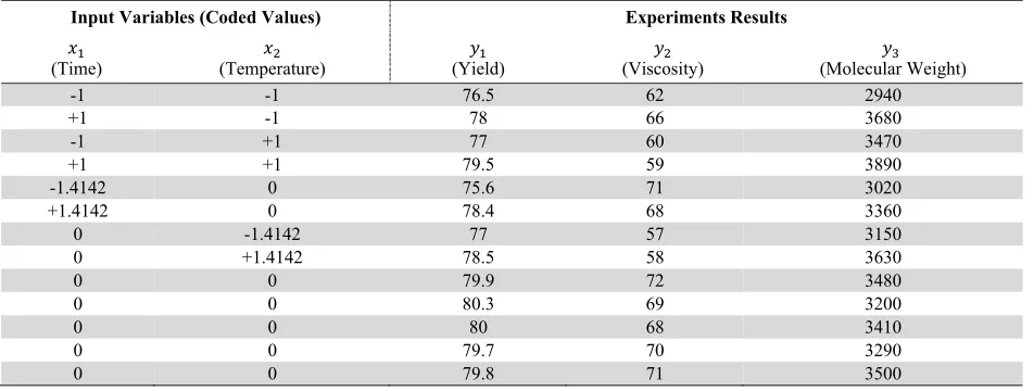
Here, in order to show the applicability of the model a chemical mixture problem is chosen due to applicability of this model in different aspects of engineering such as chemical, oil, and food production. So, let use the numerical case which was taken from Myers et al. (2016) and has been used by He et al. (2010). For this chemical process, two input variables (time and temperature) and three responses (yield, viscosity, and number average of molecular weight) are assumed. The first step is to construct the required experiments and collect the necessary data through running the designed experiments. Here the central composite design is used for designing experiments, see Table 2.
Table 2
Design of experiments and collected results (two input variables and three responses)
Input Variables (Coded Values) Experiments Results
(Time) (Temperature) (Yield) (Viscosity) (Molecular Weight)
-1 -1 76.5 62 2940
+1 -1 78 66 3680
-1 +1 77 60 3470
+1 +1 79.5 59 3890
-1.4142 0 75.6 71 3020
+1.4142 0 78.4 68 3360
0 -1.4142 77 57 3150
0 +1.4142 78.5 58 3630
0 0 79.9 72 3480
0 0 80.3 69 3200
0 0 80 68 3410
0 0 79.7 70 3290
0 0 79.8 71 3500
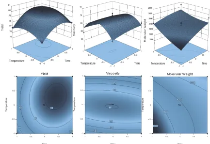
We assume all experiments were executed in the worst combination of uncertainty (environmental factors) in the problem. Note that for simplicity of the formulation, input variables are normalized in [-1, 1]. Here, the objectives are maximizing yield (LTB), minimizing molecular weight (STB), and keeping viscosity in relevant target point (NTB). The RSM is used to approximate the relationship between each response and input variables, over input/output data obtained by CCD design. The experiment results were evaluated in the Design Expert (V.10) software and the outputs. The second-order model of three responses are formulated as below:
The 3D surface and contour plot of responses are shown in Fig. 2.
Next, we add a physical constraint into a problem with the following inequality:
, : 1.37 3.25 8.70 0 (27)
The procedure of the collecting data from the production process is based on designing experiments which has been executed in the worst combinations of uncertainties (environmental variables), so, the maximum variation is imposed to each response. The procedure of robust optimization model (min-max method) has been followed in such a way that minimizes this variation (Ben-Tal et al., 2009).
79.94 0.99 0.52 0.25 1.38 1.00 (24)
70.00 0.16 0.95 1.25 0.69 6.69 (25)
3376.00 205.10 177.35 80.00 41.75 58.25 (26)
We assume, due to the existence of noises in the process, each input variable is fluctuated around its
exact value with a variance of 0.02 unit ( 0.02). We assume there is no correlation between
time and temperature, so 0. Moreover, regarding to Eq.(8) until Eq.(11), the mean and
variance of each response are approximated as below:
79.92 0.99 0.52 0.25 1.38 1.00 (28)
0.03 0.10 0.03 0.05 0.15 0.08 (29)
69.93 0.16 0.95 1.25 0.69 6.69 (30)
0.02 0.06 0.52 0.74 0.07 3.61 (31)
3376.17 205.10 177.35 80.00 41.75 58.25 (32)
1470.38 1252.55 170.13 105.60 267.45 399.45 . (33)
With the same procedure, the mean and variance of the constraint are defined as below:
1.37 3.25 8.70 (34)
0.25 1.13 0.48 1.51 1.51 (35)
We consider the production limitation for responses as 76 for yield, 60, 70 for
viscosity, and 3700 for molecular weight. The upper specification of yield is assumed four times
more than , so 304, and 925 that is four times less than upper specification.
However, the target point for all cases is estimated by ⁄ ;2 1,2,3. As
mentioned before, the quality loss coefficients play an important role for making the monetary scale in
expected losses. In the current instance, we assume 6 10 , 8, and 2 10 .
Furthermore, the expected loss function for each three responses can be approximated by following functions:
6 10 79.92 0.99 0.52 0.25 1.38 1.00 190
0.03 0.10 0.03 0.05 0.15 0.08 (36)
8 69.93 0.16 0.95 1.25 0.69 6.69 65 0.02
0.06 0.52 0.74 0.07 3.61 (37)
2 10 3376.17 205.10 177.35 80.00 41.75
58.25 2312.5 1470.38 1252.55 170.13
105.60 267.45 399.45
(38)
If we assume , 0 for the current condition, so the capabilities are 0.345, 0.338 and
0.435. The decision maker wish to reach 20 percent improvement in the performance of process for each quality characteristic. Thus, the new goals for performances are 0.432 for yeild,
0.422, and 0.543. Thus, according to Eqs.(13-15), the target point for each response is computed
as 51, 142, and 264. So, the overall objective with Lp metric method is
formulated as follow:
51 142 264 (39)
P 2 is considered for this model to show the emphasizing of the model in the amount of deviation from
the target point. The terms of , and depict the importance of each response compared to others,
and for the current instance we examine different combinations of , and .
is followed by 120 50 35 15 , and total budget allocated to process for production is 150. Also, the penalty factors which associated to the physical constraint is 2.
Model I: Robust optimization model based on overall expected loss in the process
min 51 142 264 (40)
subject to: 120 50 35 15 150 (41)
1.37 3.25 8.70 2 0.25 1.13 0.48 1.51 1.51 0 (42)
0.98 , 0.98 (43)
Model II: robust optimization model based on production cost in the process:
min 120 50 35 15 (44)
subject to: 51 142
264 20
(45)
1.37 3.25 8.70 2 0.25 1.13 0.48 1.51 1.51 0 (46)
0.98 , 0.98 (47)
We assume the value of 20 for the upper bound of overall expected loss. This threshold can be
settled based on the importance of the maximum distances between expected loss and the relevant target point for warranty the existence of feasible solutions.
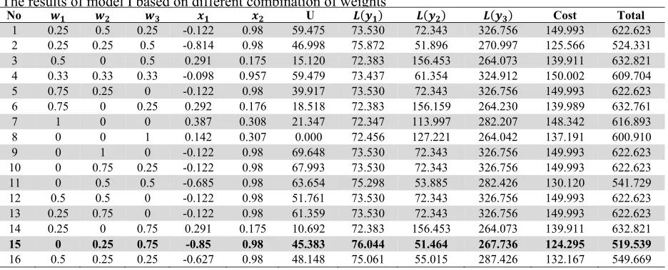
Table 3
The results of model I based on different combination of weights
No U Cost Total
1 0.25 0.5 0.25 -0.122 0.98 59.475 73.530 72.343 326.756 149.993 622.623
2 0.25 0.25 0.5 -0.814 0.98 46.998 75.872 51.896 270.997 125.566 524.331
3 0.5 0 0.5 0.291 0.175 15.120 72.383 156.453 264.073 139.911 632.821
4 0.33 0.33 0.33 -0.098 0.957 59.479 73.437 61.354 324.912 150.002 609.704
5 0.75 0.25 0 -0.122 0.98 39.917 73.530 72.343 326.756 149.993 622.623
6 0.75 0 0.25 0.292 0.176 18.518 72.383 156.159 264.230 139.989 632.761
7 1 0 0 0.387 0.308 21.347 72.347 113.997 282.207 148.342 616.893
8 0 0 1 0.142 0.307 0.000 72.456 127.221 264.042 137.191 600.910
9 0 1 0 -0.122 0.98 69.648 73.530 72.343 326.756 149.993 622.623
10 0 0.75 0.25 -0.122 0.98 67.993 73.530 72.343 326.756 149.993 622.623
11 0 0.5 0.5 -0.685 0.98 63.654 75.298 53.885 282.426 130.120 541.729
12 0.5 0.5 0 -0.122 0.98 51.761 73.530 72.343 326.756 149.993 622.623
13 0.25 0.75 0 -0.122 0.98 61.359 73.530 72.343 326.756 149.993 622.623
14 0.25 0 0.75 0.291 0.175 10.692 72.383 156.453 264.073 139.911 632.821
15 0 0.25 0.75 -0.85 0.98 45.383 76.044 51.464 267.736 124.295 519.539
16 0.5 0.25 0.25 -0.627 0.98 48.148 75.061 55.015 287.426 132.167 549.669
5. Results and discussion
have been compared in Tables 3 and Table 4 while 0 , , 1 and 1.As can be seen from the results, choosing the best solutions for this problem strongly depends on the appropriate
combinations of weighting , and which are determined by the decision maker. However,
according to first model (see again Table 3), the best result can be achieved when the first expected loss has the zero weight, and second and third expected losses are 0.25 and 0.75, respectively. In this
condition, the best result is 0.85, 0.98 and the minimum value is obtained for summation
of cost and expected losses by 519.539. By turning to second model (see Table 4), the feasibility of solutions is strongly related to the value of D (upper bound of overall expected loss). It can be seen, a
minimum total cost and losses is reached when 0.091 and 0238. In this point just the first
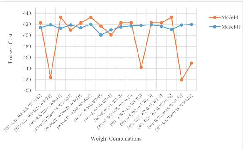
objective proceeds in overall Lp metric function (i.e. the weight one is allocated to yield’s expected loss and two others, viscosity and molecular weight are weighted zero). In general, in terms of lower total expected losses and production cost, the first model shows the better performance than the second model, while in term of robustness (i.e. variability of results due to changing in the weight combinations) the second model gives more robust results, see Fig. 3. Notably, the obtained results significantly depend on allocating magnitudes of D and B (total budget allocated to process) in model. It must be mentioned that input factor levels can determine how big of a change in the response can be gotten. Moreover, for the current instance to ensure the adequate change of each expected loss to be moved as close as possible to the target point, the bounds of changing in levels of input factors must be chosen far enough apart to make the adequate change in responses.
Table 4
The results of model II based on different combination of weights
No Cost Total
1 0.25 0.5 0.25 -0.965 0.98 120.230 72.706 194.599 226.573 614.108
2 0.25 0.25 0.5 -0.158 0.347 125.075 72.706 194.599 226.573 618.953
3 0.5 0 0.5 -0.98 0.958 118.622 72.706 194.599 226.573 612.500
4 0.33 0.33 0.33 -0.163 0.348 124.863 72.706 194.599 226.573 618.741
5 0.75 0.25 0 -0.98 0.98 119.706 72.706 194.599 226.573 613.584
6 0.75 0 0.25 -0.412 0.649 126.105 72.706 194.599 226.573 619.983
7 1 0 0 -0.091 -0.238 106.813 72.706 194.599 226.573 600.691
8 0 0 1 -0.98 0.908 116.143 72.706 194.599 226.573 610.021
9 0 1 0 -0.252 0.361 121.391 72.706 194.599 226.573 615.268
10 0 0.75 0.25 -0.203 0.354 123.303 72.706 194.599 226.573 617.181
11 0 0.5 0.5 -0.18 0.351 124.205 72.706 194.599 226.573 618.083
12 0.5 0.5 0 -0.173 0.349 125.205 72.706 194.599 226.573 619.083
13 0.25 0.75 0 -0.223 0.357 122.542 72.706 194.599 226.573 616.420
14 0.25 0 0.75 -0.98 0.922 116.839 72.706 194.599 226.573 610.717
15 0 0.25 0.75 -0.165 0.348 124.787 72.706 194.599 226.573 618.665
16 0.5 0.25 0.25 -0.14 0.344 125.748 72.706 194.599 226.573 619.626
6. Conclusion
References
Ardakani, M. K., & Noorossana, R. (2008). A new optimization criterion for robust parameter design - The case of target is best. International Journal of Advanced Manufacturing Technology, 38(9), 851– 859.
Ben-Tal, A., Ghaoui, L. El, & Nemirovski, A. (2009). Robust optimization.
Bertsimas, D., Brown, D. B., & Caramanis, C. (2011). Theory and Applications of Robust Optimization.
SIAM Review, 53(3), 464–501.
Beyer, H. G., & Sendhoff, B. (2007). Robust optimization - A comprehensive survey. Computer Methods
in Applied Mechanics and Engineering, 196(33), 3190–3218.
Boyaci, A. I., Hatipoglu, T., & Balci, E. (2017). Drilling process optimization by using fuzzy-based multi-response surface methodology. Advances in Production Engineering & Management, 12(2), 163.
Chan, L. K., Cheng, S. W., & Spiring, F. A. (1988). A New Measure of Process Capability: Cpm. Journal
of Quality Technology, 20(3), 162–175.
Charnes, A., & Cooper, W. W. (1977). Goal programming and multiple objective optimizations.
European Journal of Operational Research, 1(1), 39–54.
Chen, H.-W., Wong, W. K., & Xu, H. (2012). An augmented approach to the desirability function.
Journal of Applied Statistics, 39(3), 599–613.
Chen, W., Wiecek, M. M., & Zhang, J. (1999). Quality utility : a Compromise Programming approach to robust design. Journal of Mechanical Design, 121(2), 179–187.
Chinchuluun, A., & Pardalos, P. M. (2007). A survey of recent developments in multiobjective optimization. Annals of Operations Research, 154(1), 29–50.
Costa, N. R., Louren, J., & Pereira, Z. L. (2011). Desirability function approach: A review and performance evaluation in adverse conditions. Chemometrics and Intelligent Laboratory Systems,
500 520 540 560 580 600 620 640
Loss
es
+Cost
Weight Combinations
Model-I Model-II
107(2), 234–244.
Deb, K. (2011). Multi-objective optimization using evolutionary algorithms: an introduction, 3–34. Gabrel, V., Murat, C., & Thiele, A. (2014). Recent advances in robust optimization: An overview.
European Journal of Operational Research, 235(3), 471–483.
He, Z., Wang, J., Jinho, O., & H. Park, S. (2010). Robust optimization for multiple responses using response surface methodology. Applied Stochastic Models in Business and Industry, 26, 157–171.
Hwang, C. L., & Masud, A. S. M. (2012). Multiple objective decision making—methods and
applications: a state-of-the-art survey (Vol. 164). Springer Science {&} Business Media.
Khan, J., Teli, S. N., & Hada, B. P. (2015). Reduction Of Cost Of Quality By Using Robust Design : A Research Methodology. International Journal of Mechanical and Industrial Technology, 2(2), 122– 128.
Lukic, D., Milosevic, M., Antic, A., Borojevic, S., & Ficko, M. (2017). Multi-criteria selection of
manufacturing processes in the conceptual process planning. Advances in Production Engineering
And Management, 12(2), 151–162.
Marler, R. T., & Arora, J. S. (2004). Survey of multi-objective optimization methods for engineering.
Structural and Multidisciplinary Optimization, 26(6), 369–395.
Messac, A., & Ismail-Yahaya, A. (2002). Multiobjective robust design using physical programming.
Structural and Multidisciplinary Optimization, 23(5), 357–371.
Miettinen, K. (2001). Some methods for nonlinear multi-objective optimization. Evolutionary
Multi-Criterion Optimization, 1–20.
Miettinen, K. M. (2012). Nonlinear multiobjective optimization (Vol. 12). Springer Science {&} Business Media.
Myers, R., C.Montgomery, D., & Anderson-Cook, M, C. (2016). Response Surface Methodology:
Process and Product Optimization Using Designed Experiments-Fourth Edittion. John Wiley & Sons.
Nha, V. T., Shin, S., & Jeong, S. H. (2013). Lexicographical dynamic goal programming approach to a robust design optimization within the pharmaceutical environment. European Journal of Operational
Research, 229(2), 505–517.
Park, C., & Leeds, M. (2016). A Highly Efficient Robust Design Under Data Contamination. Computers {&} Industrial Engineering, 93, 131–142.
Park, S., & Antony, J. (2008). Robust design for quality engineering and six sigma. World Scientific Publishing Co Inc.
Parkinson, A., Sorensen, C., & Pourhassan, N. (1993). A general approach for robust optimal design.
Journal of Mechanical Design, Transactions of the ASME, 115(1), 74–80.
Parnianifard, A., Azfanizam, A. S., Ariffin, M. K. A., & Ismail, M. I. S. (2018). An overview on robust
design hybrid metamodeling : Advanced methodology in process optimization under uncertainty.
International Journal of Industrial Engineering Computations, 9(1), 1–32.
Phadke, M. S. (1989). Quality Engineering Using Robust Design. Prentice Hall PTR.
Sahali, M. A., Serra, R., Belaidi, I., & Chibane, H. (2015). Bi-objective robust optimization of machined surface quality and productivity under vibrations limitation. In MATEC Web of Conferences (Vol. 20). EDP Sciences.
Sharma, N. K., & Cudney, E. A. (2011). Signal-to-Noise ratio and design complexity based on Unified
Loss Function – LTB case with Finite Target. International Journal of Engineering, Science and
Technology, 3(7), 15–24.
Sharma, N. K., Cudney, E. A., Ragsdell, K. M., & Paryani, K. (2007). Quality Loss Function – A Common Methodology for Three Cases. Journal of Industrial and Systems Engineering, 1(3), 218– 234.
Simpson, T. W., Poplinski, J. D., Koch, P. N., & Allen, J. K. (2001). Metamodels for Computer-based Engineering Design: Survey and recommendations. Engineering With Computers, 17(2), 129–150. Wang, G., & Shan, S. (2007). Review of Metamodeling Techniques in Support of Engineering Design
Optimization. Journal of Mechanical Design, 129(4), 370–380.
Zadeh, L. (1963). Optimality and non-scalar-valued performance criteria. Automatic Control, IEEE