Evaluating the performance of a new classifier – the GP-OAD:
A comparison with existing methods for classifying rock type
and mineralogy from hyperspectral imagery
Sven Schneider
⇑, Richard J. Murphy, Arman Melkumyan
Australian Centre for Field Robotics, The Rose Street Building, J04, Department of Aerospace, Mechanical and Mechatronic Engineering, University of Sydney, NSW, Australia
a r t i c l e
i n f o
Article history: Received 8 January 2014
Received in revised form 30 September 2014
Accepted 30 September 2014 Available online 11 November 2014 Keywords: Hyperspectral Absorption feature Iron minerals Vertical geology Illumination conditions Machine learning Classification Remote sensing
a b s t r a c t
In this study, we compare three commonly used methods for hyperspectral image classification, namely Support Vector Machines (SVMs), Gaussian Processes (GPs) and the Spectral Angle Mapper (SAM). We assess their performance in combination with different kernels (i.e. which use distance-based and angle-based metrics). The assessment is done in two experiments, under ideal conditions in the labora-tory and, separately, in the field (an operational open pit mine) using natural light. For both experiments independent training and test sets are used. Results show that GPs generally outperform the SVMs, irrespective of the kernel used. Furthermore, angle-based methods, including the Spectral Angle Mapper, outperform GPs and SVMs when using distance-based (i.e. stationary) kernels in the field experiment. A new GP method using an angle-based (i.e. a non-stationary) kernel – the Observation Angle Dependent (OAD) covariance function – outperforms SAM and SVMs in both experiments using only a small number of training spectra. These findings show that distance-based kernels are more affected by changes in illumination between the training and test set than are angular-based methods/kernels. Taken together, this study shows that independent training data can be used for classification of hyperspectral data in the field such as in open pit mines, by using Bayesian machine-learning methods and non-stationary kernels such as GPs and the OAD kernel. This provides a necessary component for automated classifications, such as autonomous mining where many images have to be classified without user interaction.
Ó2014 The Authors. Published by Elsevier B.V. on behalf of International Society for Photogrammetry and Remote Sensing, Inc. (ISPRS). This is an open access article under the CC BY-NC-ND license (http://creati-vecommons.org/licenses/by-nc-nd/3.0/).
1. Introduction
To characterise rock type or mineralogy, hyperspectral data have been acquired in the laboratory (e.g.Cudahy et al., 2009; Doublier et al., 2010; Huntington et al., 2004), from satellite and airborne platforms (Brown, 2006; Swayze et al., 2009; Goetz, 2009) and from field-based platforms (Kruse et al., 2011; Kurz et al., 2008, 2011; Murphy et al., 2012). Such data are of sufficient spectral resolution to resolve broad crystal field absorptions in the visible and near-infrared (VNIR) as well as narrower absorption features caused by vibrational processes in the short-wave infrared (SWIR, Hunt and Salisbury, 1970; Rencz, 1999). Traditionally, methods to identify materials, including minerals, from hyperspectral data characterise specific absorption features within the spectral curve. Methods operating on the level of individual absorption fea-tures – ‘‘feature-based methods’’ – rely on extraction of attributes
from these features, e.g. their wavelength position, depth and width (Clark et al., 1990, 2003; Murphy et al., 2014a, b, c; Zaini et al., 2014). Extraction of these attributes may, however, be problematic in cases where absorption features are masked by noise or by other, more dominant, features (e.g.Swayze et al., 2003; Rodger et al., 2012).
In recent years, machine-learning methods (often supervised methods) for classification of hyperspectral data (e.g. Support Vector Machines) have received increasing attention (e.g.Bazi and Melgani, 2006; Alajlan et al., 2012; Foody and Mathur, 2004; Plaza et al., 2009 and references therein). Kernel machines such as SVMs have opened up the possibility of using flexible models which are practical to work with (Mountrakis et al., 2011). Machine-learning methods often use all the spectral bands in the dataset, however, methods are also used to reduce the volume of data (e.g.Demarchi et al., 2014). Processing of these large amounts of information is possible by applying convenient mathematical formulations to the data such as the ‘‘kernel trick’’ (Smola and Schölkopf, 2004). Other machine learning methods, e.g. Gaussian http://dx.doi.org/10.1016/j.isprsjprs.2014.09.016
0924-2716/Ó2014 The Authors. Published by Elsevier B.V. on behalf of International Society for Photogrammetry and Remote Sensing, Inc. (ISPRS). This is an open access article under the CC BY-NC-ND license (http://creativecommons.org/licenses/by-nc-nd/3.0/).
⇑ Corresponding author. Tel.: +49 176 569 823 15. E-mail address:[email protected](S. Schneider).
Contents lists available atScienceDirect
ISPRS Journal of Photogrammetry and Remote Sensing
j o u r n a l h o m e p a g e : w w w . e l s e v i e r . c o m / l o c a t e / i s p r s j p r sProcesses (GPs; Rasmussen and Williams, 2006), have been successfully applied to classification of multi- and hyperspectral data and in the selection of spectral bands and retrieval of biophysical properties (e.g. Bazi and Melgani, 2008; Pasolli et al., 2010; Verrelst et al., 2012). Recent studies report a competitive classification performance of GPs compared to SVMs (e.g. Bazi and Melgani, 2010).
Many studies using supervised machine-learning methods lack, however, a thorough assessment of the performance of these methods in general terms because they are often limited to (i) sim-ulated data, (ii) using cross-validation to validate the performance of the algorithm and/or (iii) using non-independent training and test sets where the training and test data are often selected from the same population of data. These approaches do not provide a general test of the performance of methods, leading to an overop-timistic assessment of the performance of these methods for data acquired from different scenes or under different environmental conditions. This is because training and test data are often: (i) acquired at the same time of the same target, (ii) under the same physical conditions, (iii) with the same sensor and (iv) using the same sensor parameters (e.g.Jiang et al., 2007; Monteiro et al., 2009; Li et al., 2011). Therefore, applications of methods using such data tend to remove any extraneous factors which are contained within a particular image. This approach works but generally requires specifying training data manually, which may be a difficult and laborious process and which is incompatible with automated tasks of classification. For example, it constrains the use of supervised methods in autonomous operational mining where many images of different surfaces need to be classified using data acquired from airborne and field-based platforms. The use of an independent spectral library or training set is therefore necessary to enable methods to be applied consistently and automatically across imagery acquired from different targets. Given these requirements, there is a need to compare methods for classification of hyperspectral data when training data and test data come from different (i.e. independent) populations of data. Only then can we make statements about the general performance of methods.
Few studies have evaluated the performance of supervised machine-learning methods using independent training and test sets (but seeNidamanuri and Zbell, 2011a, b). Because SVMs and GPs are increasingly being used in remote sensing applications and research, a comparison of these methods under more rigorous experimental conditions is timely. This study differs from previous studies by providing a rigorous test of methods by using indepen-dent training and test data, without the use of cross-validation. Independent in the context means that training and test data are not derived from the same data set or image and are not acquired by the same sensor. Training and test data are acquired using different sources of illumination (artificial vs natural) and different types of sensors (non-imaging and imaging spectrometers). In this study, a new method of classification of hyperspectral data – the GP-OAD (Schneider et al., 2010) – is compared against the Radial Basis Function (RBF) kernel, SVMs and the Spectral Angle Mapper (SAM, Kruse et al., 1993). Previous studies have indicated that the performance of the GP-OAD is superior to other methods (e.g.Chlingaryan et al., 2013; Schneider et al., 2011) but this has not yet been formally tested.
A two-stage validation strategy was developed which compared the aforementioned methods first using data acquired in the laboratory under stable artificial illumination and then using imagery of a mine face in an open pit mine, acquired under natural illumination. This two-staged approach was necessary because findings from laboratory studies cannot be assumed to have relevance when methods are applied to data acquired in the field under natural light. This is because imagery acquired in the field is affected by spatial variability in illumination, including shade
and effects of the intervening atmosphere. Absorption by water vapour across certain wavelength regions (e.g. those centred on 720 nm, 762 nm, 822 nm, 945 nm 1135 nm) can reduce amounts of incident light causing a lower signal-to-noise ratio (SNR) close to these wavelengths. Other environmental and measurement effects can also have a significant impact on the quality of imagery acquired in the field (reviewed byKurz et al., 2013). It is, therefore, of fundamental importance to understand any differences in the results obtained from laboratory and field data. Only then can we make general statements about the suitability of methods for classification of hyperspectral data acquired from satellite, airborne and field based platforms.
2. Materials and methods
2.1. Study area and geological setting
The study area from which exploration drill cores and field imagery were obtained, was an operational open pit mine in the Pilbara, Western Australia. The area is characterised by extensive areas of banded iron formation (BIF) comprised of alternating layers of silica (often chert; CHT) with hematite or magnetite. Some areas have become mineralised through the influence of weathering and ground-water leaching. In this process, silica, a major component of CHT and BIF, is leached from the rock matrix, concentrating deposits of iron in the form of goethite and martite (hematite). Other major rock types in this area are different types of shales, including thin volcanic shale bands (SHL2), extensive deposits of West Angeles Shale (SHL1) and another type of shale (SHL3), containing variable amounts of kaolinite and/or halloysite, with bands of pyrolusite. Mineralised areas contain iron-rich materials dominated by goethite–limonite (GOL) which has a high abundance of goethite and a mixture of martite–goethite (MAR) which is abundant in both minerals but generally has a higher content of martite. The particular mine face used in this study exhibits all of these rock types. Mining is conducted via conven-tional drill and blast open-pit operations. The training set/spectral library was acquired from exploration drill-core samples from this area. The test data were acquired from the same drill cores (Experiment 1), however, spatially independent from the training set and from bulk rocks on a mine face (Experiment 2).
2.2. Data acquisition 2.2.1. Sensors
Hyperspectral data were acquired using two different sensors. A field spectrometer (Analytical Spectral Devices, Boulder, Colorado; ASD) was used to acquire reflectance spectra (350–2500 nm) for the spectral library. This spectrometer has a spectral sampling interval of 1.4 and 2 nm Full Width at Half Maximum (FWHM) for the VNIR and 3 and 10 nm, respectively, for the two SWIR sensors. Data were digitised at 16 bits and the fibre-optic of the device was fitted with an 8°fore-optic. Two imaging spectrometers (Specim, Finland) were used to acquire data from exploration drill cores in the laboratory and of a mine face in the field. The VNIR (400–1027 nm) and SWIR (971–2516 nm) imagers had a FWHM spectral resolution of 4.6 and 6.4 nm, respectively digitised at 12 and 14 bits.
2.2.2. Spectral library
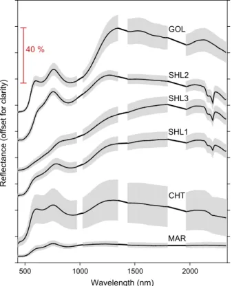
This spectral library is the ‘reference’ or ‘training’ library used for the different classification methods in all experiments (Fig. 1). It is comprised of 90 spectra unevenly distributed across 6 classes of rock (Table 1). The spectral library was constructed from drill cores (10 cm wide) using artificial illumination and a consistent
target-sensor-illumination geometry (Schneider et al., 2009). A reference spectrum was acquired using a calibration panel (99% Spectralon) prior to each target measurement. Each reflectance spectrum was comprised of an average of 25 individual spectral measurements. Spectra were converted to absolute reflectance by dividing the target spectrum by the calibration spectrum and multiplying this quotient by the factors of the calibration panel. For consistency across all experiments, ASD spectra were converted to the band-passes of the imaging sensor using Gaussian convolution. In addition, spectral bands around the major water absorption bands centred at about 1400 and 1900 nm were removed. Each library spectrum processed in this way comprised 283 spectral bands.
2.2.3. Laboratory imagery
The drill cores exhibited mainly smooth and dust free surfaces and were stored in plastic trays. Trays were comprised of four cores (each approximately 1 m in length), each core being
separated from a neighbouring core by a plastic divider. The imaging sensors were mounted on a scanning frame, nadir to the target. The distance from the target to the sensors was860 mm. To minimise shading effects, core trays were illuminated using two arrays of seven halogen lamps each, illuminating the tray at an angle of ±45°from each side. The halogen lamps were approximately 40 cm away from the cores. A calibration panel (99% Spectralon), covering the entire spatial dimension of the sensor array, was placed into the field of view of the sensors at the beginning of each tray.
A correction was applied to the image spectrum at each pixel in the VNIR images to remove an artefact (an increase in reflectance towards shorter wavelengths), caused by frame-smear. Dark cur-rent was then subtracted from each VNIR and SWIR images on a line-by-line basis. The calibration panel was used to calibrate the images to reflectance on a line-by-line basis. To maximise the SNR in the image spectra, separate calibration and target images, were acquired using integration times that allowed the full dynamic range of each sensor to be used. The difference in integra-tion time of the two images was taken into account during the reflectance calibration using Eq.(1):
q
ðkÞtray¼ DNðkÞtrayq
0ðkÞWR DNðkÞWR ttray tWR ; ð1Þwhere
q
(k)trayis the reflectance of a tray image at bandk,DN(k)tray is the digital number of an individual pixel in the tray image, DN(k)WR is the line average of forty image frames of the white reference andq
0(k)WR is the reflectance factor of the calibration panel at the wavelength k. Integration times for the calibration image and the tray image are indicated bytWRandttray, respectively. Image spectra showed large increases in noise due to reduced sensor sensitivity towards the shorter (400–439 nm) and longer (>970 nm) end of the VNIR sensor. Noise also affected the shorter end of the SWIR sensor (971–1027 nm) and wavelengths longer than 2335 nm. Thus, these bands (and the small spectral overlap between the VNIR and SWIR sensors) were removed from the image cubes. The same was done for the training set to have the same number of bands in both data sets (283 bands). The VNIR and SWIR images were spatially registered using interpolation.
Sixteen trays of drill cores were acquired and processed in this way. A meta-data set was then constructed for this study by extracting six rock types across all images (Table 1). Several rock samples of each of the six rock types were combined into a single hyperspectral image (Fig. 2).
Because it is difficult to determine the identity of what mineral or composite suite of minerals which make up rock samples simply by colour/appearance alone, samples for X-ray diffraction analysis (XRD) were acquired from the rock samples after acquisition of spectral data (Ramanaidou et al., 2008). To provide a more definitive labelling of areas of the core we used XRD results in combination with visual inspection and contextual placement of each area within the core relative to other areas. This enabled us to determine if the assigned labels on the core were consistent with the measured and expected mineralogy.
Wavelength (nm)
500 1000 1500 2000
Reflectance (offset for clarity)
40 % GOL SHL2 MAR CHT SHL3 SHL1
Fig. 1.Average spectra (black lines) of the 6 rock types in the library. The standard deviation per band is shown as grey areas around the mean. Bands close to the junction sensed by the separate VNIR and SWIR sensors have been removed as were bands affected by atmospheric water near 1400 and 1900 nm. In the figure, bands next to the gaps are connected with straight lines for clarity. The indicator is included for scale, indicating the magnitude of the different spectra. (For interpre-tation of the references to colour in this figure legend, the reader is referred to the web version of this article.)
Table 1
Overview of the training data (spectral library) used for training and classification. The uneven number of spectra was due to variable surficial areas of rock being available among the classes for spectral analysis.
Rock type Acronym Description N spectra
Cherty BIF CHT An extreme silicic version of Banded Iron Formation (BIF). Chert (silica). Very hard, light crème brown to yellow 8
Martite–goethite MAR Soft to hard texture, red–brown, black–grey 18
Goethite–limonite GOL Ochreous goethite – chalky in appearance. Yellow to brown 17
Shale 1 SHL1 Shale, soft. Pink to yellow, kaolinitic 13
Shale 2 SHL2 Volcanic shale. Soft. Light cream, pinkish, kaolinitic 12
2.2.4. Field imagery
Hyperspectral imagery was acquired from the mine face using the VNIR and SWIR sensors mounted adjacently on a rotating stage (Fig. 3). A calibration panel (60% Spectralon; 30 cm by 30 cm), was placed next to the mine face during image acquisition. Integration times of the sensors were adjusted so that the brightest object of interest within the scene did not saturate. The VNIR and SWIR imagery were spatially registered and corrected for dark current in the same way as the laboratory imagery. Reflectance calibration was done on a band-by-band basis by dividing each pixel by the average value of pixels over the calibration panel and multiplying by the reflectance factors of the panel. The final image cube had a spatial resolution of 1882 by 291 pixels with 283 bands. The spatial resolution per pixel was 4.8 cm.
2.3. Gaussian Processes (GPs)
A Gaussian Process (GP) in a supervised learning problem uses a given training setD= (X,y) consisting of a matrix of training data X= [x1,x2,. . .,xN]T, whereTindicates a transposed vector or matrix and y= [y1,y2,. . .,yN]T, consisting of Ninput points (i.e. training samples). To each vector xi2RB, with i= 1, 2, . . ., N, a target yi
e
{1, 1} is associated. The vector xi in this context is a reflectance spectrum within the training dataX (i.e. the spectral library) with B number of spectral bands. The predictive distributionf(x⁄) at a new test pointx⁄(i.e. a reflectance spectrum of an unknown class) can then be computed. A GP model uses a multivariate Gaussian distribution over the space of function variables f(x) mapping input to output spaces. A GP is fully specified by its mean function m(x) and covariance function k(x, x0), so fðxÞ GPðmðxÞ;kðx;x0ÞÞ. Using ðX;f;yÞ ¼ fxig;ffig; ð
fyigÞ N
i¼1 for the training set (i.e. a spectral library consisting of
reflectance data) and Xð ;f;yÞ ¼ fxig;ffig;fyig
N
i¼1 for a test
point (i.e. a pixel in a reflectance image), the joint Gaussian distribution withm(x) = 0 becomes:
y f N 0; KðX;XÞ þ
r
2 KðX;X Þ KðX;XÞ KðX;XÞ " #! : ð2ÞN ð
l
;RÞis a multivariate Gaussian distribution with meanl
and covarianceRand K is the covariance matrix computed between all points in the data set. By conditioning on the observed training points, the predictive distribution for new points (i.e. spectra constituting pixels in a reflectance image) can be obtained by p fðijX;X;yÞ ¼ N ðl
;RÞwherel
⁄andR⁄are the new mean and covariance for the test data.2.3.1. Learning hyper-parameters
Learning (or training) a GP model is equivalent to learning the hyper-parameters of the covariance function (kernel) from a data set. In a Bayesian framework this can be performed by maximizing the log of the marginal likelihood with respect to the hyper-parameters which control data-fitting and regularisation of the model. The trade-off between regularisation and data-fit in the GP model is automatic, i.e. no manual parameter tuning is necessary. In this study, the hyper-parameters were initialized with random values and a gradient descent method was used to search for their optimal values (i.e. a global minimum). To avoid converging to a local minimum, the search step was repeated several times with different random starting points in the hyper-parameter space (Williams and Rasmussen, 1996). After this step, the best parameter set was selected by comparing the magnitude of the log marginal likelihood for each starting point and selecting the one with the largest value.
2.3.2. Predicting class probabilities for hyperspectral imagery Prediction of class probabilities for a test sample x⁄ (i.e. an image pixel) is obtained from the joint Gaussian distribution of the training samples and the test samples by conditioning on the observed targets in the training set. Generally, the predictive distribution is Gaussian with a mean and a covariance function. Using Bayesian inference, the most likely label for a samplex⁄with some uncertainty around it can be obtained. These two parameters are equivalent to the mean (
l
) and the standard deviation (r
) of a Gaussian distribution and can thus be used to calculate the probability of a pixel belonging to either the ‘One’ or the ‘All’ class using the Gaussian cumulative distribution function. The result is the probability that a single observation from a normal distribution with parametersl
andr
will fall in the interval (1, 0] because labels in our implementation of the ‘One versus All’ (OvA) classification were set to ‘1’ (‘One’ class) and ‘1’ (‘All’ class). 2.4. Support Vector Machines (SVMs)Our implementation of SVMs, outlined here, is derived from the work ofVapnik (2000) and similar toMurphy et al. (2012). To perform classification, the standard procedure is to apply a hard decision function to the final SVM. Because results obtained using hard decision boundaries were poor, we adopted an alternative
Fig. 2.Composite image using red, green and blue bands. The pixel resolution of this image was 0.11 cm.
Fig. 3.Contrast-enhanced true-colour composite with overlaid geological boundaries mapped in the field. Geological zones are indicated by numbers: (1) shale1; (2) shale2; (3) mixed goethitic shale and ore (GOL and possibly MAR); (4) ore zone (GOL with MAR background); (5) ore zone (dominant MAR with GOL background); (6) ore zone (GOL); (7) ore zone – dominant MAR, with background CHT. Shaded areas indicated by ‘‘S’’. Black dotted line marks the boundary between rill (loose rocks) and the ore-body. The material in zone 4 below the rill-line and the right part of zone 5 below the rill-line is mainly composed of SHL1 with some GOL. The sky in the image and the road below the mine face are masked out (black in the image).
approach that makes use of probabilistic estimates of class membership. Probabilistic predictions are particularly useful for problems having more than two classes, as is the case here. The decision is made based on a winner-takes-all strategy, i.e., the winning class is the one with the highest probability. To obtain probabilistic estimates, we transformed the SVM output to represent the likelihood of class membership, as inPlatt (1999). The probabilities were obtained by fitting a parametric model to the output of the SVM; the parameters were calculated by the numerical optimization method proposed inLin et al. (2007). They used essentially the same algorithm asPlatt (1999), however, they improved their method in terms of numerical robustness using Newton’s method and back-tracking (Nocedal and Wright, 2006). In order to provide a fair test of methods, in which no manual parameter tuning was performed, the SVM regularisation parameterCwas set to 1.
2.5. Covariance functions (kernels)
Covariance functions or kernels can be used within several kernel machines (e.g. SVMs and GPs) without adapting the kernel to a given method or framework if they conform to the Mercer’s theorem (Schoelkopf et al., 1999). The following two kernels used in this study conform to the Mercer’s theorem (Table 2).
The GP framework requires computing the covariance between all input pairs xand x0 (i.e. between spectra) or alternatively a covariance function which correlates the data in order to learn hyper-parameters and perform inference. A kernel can be combined with the GP framework by replacing the square brackets in Eq.(2)with any kernel, so that it becomes y
f ~N ð0;kOADÞand y f
~N ð0;kSEÞ, respectively for the two kernels presented in this study.
2.5.1. The Observation Angle Dependent (OAD) kernel
The OAD kernel (Melkumyan and Nettleton, 2009) computes the covariance between spectra using an angular metric and depends, not on the differencex–x0, but on the spatial location of the points xand x0, thus the OAD kernel is non-stationary. The OAD is defined as:
kOADðx;x0Þ ¼
r
20 1 1sinu
p
a
ðx;x 0Þ ; ð3Þwhere
r0
andu
are scalar hyper-parameters of the kernel anda
(x,x0) represents the spectral angle between two spectra. The parameter
u
controls the weight of the spectral angle and adjusts the influence ofa
on the overall correlation betweenxandx0;r0
is a scaling factor. Empirical tests showed that small changes on the values of the hyper-parameters have negligible effects on the classification outcome, this was however, not tested quantitatively. Both hyper-parameters were learned automatically from the training data by maximising the log of the marginal likelihood (Section 2.3.1). No manual tuning of any parameter was done, neither for the SVMs nor for GPs.2.5.2. The squared exponential or RBF kernel
The squared exponential (SE) covariance function also known as Radial Basis Function (RBF) is defined as
kSEðx;x0Þ ¼
r
20expðxx0Þ2
2l2
!
ð4Þ
Unlike the OAD kernel, the SE kernel is stationary which means that it is invariant against translation which can be seen from the nominator in Eq.(4). The signal variance
r0
is one of the hyper-parameters of this kernel and is learned from the data, representing a scaling factor. The second hyper-parameter is the characteristic length-scalelwhich determines how quickly the sample function varies and in turn controls the amount of correlation betweenxandx0. Ifxis a vector,lbecomes a vector with the same dimension-ality asxto account for the variation in each dimension. Both kernel parameters were automatically learned from the training data for the SVM and GP framework using the methods described in Sections 2.3 and 2.4, respectively.
2.6. Classification approach for machine learning methods
The following strategy was used for classifications using GPs and SVMs. For the classification of each rock type, all spectra within the training set which were of the rock type being classified, were labelled as ‘1’, other spectra from all other rock types (classes) were labelled ‘1’. The aim was to identify all samples of classes ‘1’ and ‘1’ in the unknown test set correctly. This is a binary approach of classification and is known as ‘One versus All’ or ‘One versus Rest.’ The classification algorithm is appliedntimes forndifferent classes in a data set (Rifkin and Klautau, 2004). For example, in the case of the training set used in this study comprising six classes, the algorithm had to be applied six times (Fig. 4).
Table 2
Overview of methods and kernels used in this study.
Method Kernel References
Support Vector Machine (SVMs)
OAD, SE (SVMs and SE,Vapnik, 1998) (OAD,Melkumyan and Nettleton, 2009) (SE,Bishop, 2006)
Gaussian Processes (GPs) OAD, SE (GPs,Rasmussen and Williams, 2006) See above for kernel references Spectral Angle
Mapper (SAM)
n/a (Kruse et al., 1993)
x y CC12 Cn-1 Cn z xCC12 Cn-1 Cn z means variances xC1C2 Cn-1 Cn z
Compute probabilities (P) from the means and variances for each layer (class).
Assign class labels according to the highest probabilities across the z-dimension, i.e. find highest P among the different classes.
GP-OAD Input: x z y y Outputs: compute P Result:
Fig. 4.Classification of a hyperspectral image (input) using the GP-OAD. The output of a GP – a set of means and standard deviations for each class – is obtained during inference. This set of means and standard deviations has the spatial dimensions (x, y) of a hyperspectral image and a third dimension (z) which is determined the number of class in the training set. From the means and standard deviations, a set of probabilities is calculated for each class, indicated byC1,. . .,Cn. Thereafter, class
labels are assigned according to the highest probability (result) along the z dimension, where each layer (C1,. . .,Cn) represent a class of the training set.
2.7. Spectral Angle Mapper (SAM)
SAM was selected for comparison with the machine-learning methods because it is commonly used to classify hyperspectral data; SAM is also embedded at the core of the OAD kernel. It therefore enables direct comparison of machine-learning methods with a method which does not operate within a probabilistic framework. SAM calculates the similarity of two spectra in a high dimensional space using the spectral angle
a
, Eq. (5). The brightness of a spectrum does not influence the spectral angle, i.e. the norm of a vector does not cause a change in the angle between two vectors. The spectral anglea
is calculated usinga
¼cos1 xx0kxk kx0k; ð5Þ
wherexandx0are a target and a reference spectrum, respectively. The norm of either vector is denoted by ||x|| and ||x0||.
SAM is often implemented by applying a user-specified angular threshold (e.g.Shrestha et al., 2005; Dehaan et al., 2007). Other implementations can be used to improve scene classification, for example, a ‘minimum angle’ criterion can be applied, whereby a target vector is compared to all reference spectra in a spectral library (e.g.Clark et al., 2005; Hecker et al., 2008). A class label is then assigned by comparing the angles of all target-reference combinations and selecting the class of the reference spectrum which has the smallest angle with the unknown (target) spectrum. The ‘minimum angle’ implementation of SAM was used in this paper because it has been shown to perform better than a fixed threshold implementation under certain circumstances (Murphy et al., 2012).
2.8. Quantitative assessment of classifier performance
A standard set of statistics was used to evaluate the classification performance of methods applied to laboratory data. For each classi-fication, the number of true-positive, false-positive, true-negative and false-negative classifications for each rock type was deter-mined. Statistical measures to assess classifier performance were derived from these data, including accuracy, precision, and recall. Recall measures the quantity of positive results predicted by the method. It is the number of positive results predicted divided by the total number of results that should have been returned. Precision is a measure of the quality of the results predicted and is the number of positive results predicted divided by the total number of results returned (Olson and Delen, 2008; van Rijsbergen, 1979). The F-score is defined as the harmonic mean between recall and precision, i.e. F= (2precisionrecall)/ (precision + recall). The kappa coefficient of agreement (Kappa, Congalton et al., 1983; Hudson and Ramm, 1987) was also deter-mined. A Student’sT-test was done to determine if the differences between the classification performances of the different methods were statistically significant.
2.9. Experiments
2.9.1. Experiment 1 – Comparison of methods under laboratory conditions
This experiment compared quantitatively the classification performance of the different methods under ideal conditions where data were acquired under artificial illumination in the laboratory. This enabled the SNR to be optimised across all bands and implicitly excludes effects caused by variability in incident illumination. This approach enabled a direct comparison of the inherent performance of methods because atmospheric absorption and scattering, shade and variable illumination effects (which are
present in data acquired under natural illumination) are removed from consideration. If relative strengths and weaknesses of the different methods are identified in this experiment it will help significantly in understanding results obtained in the field where ground-truth may be sparse or non-existent.
The different methods were used to classify an ‘‘unknown’’ set of data using parameters that were learned (trained) on a different, independent set of data. To ensure independence of data, the spectral library and the imagery to be classified were designed to be spatially independent. If a method fails when applied to data acquired under ‘ideal’ conditions then it would be unlikely to be successful when applied to data acquired under field conditions.
For validation, data obtained by XRD analysis were used to pro-vide quantitative information on the abundance of the different rock samples. These data were then used to validate class labels for the test and training set.
2.9.2. Experiment 2 – Comparison of methods under field conditions This experiment tested the hypothesis that different rock types in imagery acquired under natural light can be classified using training data (spectral library) acquired by a different sensor (an ASD spectrometer) using artificial illumination. For validation, the mine face was mapped thematically into different zones (Fig. 3). This division was made based on knowledge of the geology of the region and the particular mine in question. Due to safety considerations, mapping could only be done by visual inspection (e.g. colour, roughness and stratigraphy) of exposed rocks on the vertical mine face. To increase accuracy, a geologist who had an operational knowledge with this particular mine pit and its geology was used to verify this mapping.
3. Results
3.1. Experiment 1
Quantitatively, most methods achieved very high accuracies (>95%) with the exception of the SVM-SE (<90%;Fig. 5,Table 3). SAM, using the minimal angle criterion, performed well with high accuracy (97%) andF-score (90%). SAM also showed a relatively consistent classification performance across the six classes indicated by the relatively small standard deviation (error bars in Fig. 5). SAM outperformed SVM-based methods, irrespective of the kernel used.
Generally, the SVM-based methods performed poorly compared to GP-based methods in terms of accuracies andF-scores across all kernels. The OAD kernel outperformed the SE kernel in both the GP and SVM frameworks with respect to accuracy and F-score. On average, all measures showed that the GP-OAD outperformed all other methods, including SAM. The GP-OAD achieved the greatest consistency across all classes and among all classifiers as indicated by its standard deviation. The difference between the GP-OAD and SAM was, however, not statistically significant (P> 0.05).F-scores were, on average, above 90% for the GP-OAD and SAM, around 84% for the GP-SE and around 70% for both SVM kernels. The SVM-SE exhibited by far the largest inconsistencies in accuracies andF-scores, i.e. it had the largest standard deviation. For some individual rock types, the SVM-SE achievedF-scores below 50% (e.g. CHT). This performance was equivalent to a random guess considering that the classification for each rock type was done in an OvA paradigm (i.e. as a binary classification problem). The GP-OAD was significantly better (P< 0.05) than the SVM-SE, SAM was not significantly better than the SVM-SE (P> 0.05).
Overall, qualitative classifications of individual rocks using the GP-OAD (Fig. 6b) and SAM (Fig. 6d) were in good agreement with ground-truth (Fig. 6a) and were consistent with quantitative
results. The GP-SE (Fig. 6c) showed similar results to the GP-OAD and SAM, however, there was confusion between SHL1 and SHL2, causing a decrease in theF-score. A larger number of false positives for CHT caused the overall performance of the SVM-OAD to be lower than the GP-OAD’s. The rock type SHL1 was almost entirely misclassified by the SVM-OAD. This inconsistency across rock types caused the second lowest classification performance overall. The SVM-SE classified all CHT samples correctly (i.e. a very good recall was achieved), however, there was a large number of false positives for CHT (i.e. poor precision) which caused the F-score for this rock type to drop below 50%. This in turn affected the per-formance for other rock types, as many samples from other classes were misclassified as CHT, causing the poorest performance of the SVM-SE overall.
3.2. Experiment 2
Any geological zone on a mine face can never be comprised entirely of only one rock type. Thus, a classification is considered
of good quality if the dominant rock type of a geological zone (mapped during a geological survey) has been assigned to the majority of pixels in a particular zone. Although this approach does not provide an absolute measure of the performance of classifiers it provides a way of assessing the performance of each classifier relative to that of all other classifiers. It is therefore not required for a classifier to classify all pixels of a zone as the dominant rock type in order to produce a ‘good’ classification.
Classifications obtained using the GP-OAD and SAM were largely consistent with the geological/mineral map made in the field. Results obtained by these two methods were very similar in most areas of the mine face (cf.Fig. 3andFig. 7a and c). Zone 1 was mainly mapped as SHL3 with large interspersed patches of SHL1. This zone was mapped in the field as being dominantly composed of SHL1. Many places in this zone, however, were covered by a grey-toned dust which was consistent with the colour of the rocks in Zone 2 (i.e. SHL3). This may explain why this area was largely classified as SHL3 rather than SHL1. Zone 2 was classified as SHL3 which was consistent with maps made in the field. Zone 3 was classified as GOL and was also mapped as GOL and goethitic shale (SHL2) in the field. The latter was, however, not detected in this zone. Zone 4, mapped as GOL in the field, was correctly classified by the GP-OAD and SAM. Small amounts of SHL1 were also detected in the upper part, which were not detected in the field. Interactive examination of individual pixel spectra revealed that pixels in this area closely resembled library spectra of SHL1 (Fig. 8). The lower part of Zone 4 was composed of rill – a loose mixture of rock fragments and dust – and was correctly classified as mostly SHL1. Zone 5, mapped in the field as MAR was largely misclassified as CHT, GOL and small amounts of SHL2 by SAM. The GP-OAD detected slightly more MAR and less SHL2 than did SAM. Zone 6 (GOL) was classified correctly by both methods. The left side of Zone 7 was largely and correctly classified as MAR with some CHT in the background by GP-OAD and SAM. The GP-OAD and SAM classified some pixels as SHL1; additionally, SAM also classified some pixels as GOL in this zone. The right side of Zone 7 (close to Zone 6) was correctly classified as GOL by both methods. Areas of Zone 7, which were shaded (marked with ‘‘S’’) were incorrectly classified as CHT.
The performance of the GP-SE was overall relatively poor. Zone 1 was classified as SHL3 with small patches of SHL1, however, large areas were incorrectly classified as GOL. Zone 2 was generally classified correctly, except for the patches of MAR. Zones 3, 4 and 6 were classified as MAR, however, these areas should have been GOL. Zone 5 was mostly classified correctly as MAR except for small patches of SHL1, CHT and SHL2. The middle of Zone 7 was classified correctly as MAR, however, the majority of this zone, i.e. the left and right sides of this zone were poorly classified.
Both SVM classifications gave very different results to those obtained by the GP-OAD and SAM. The SVM-OAD misclassified most of Zone 1, only small patches of SHL3 were correctly classified. Zone 2 was only partly classified correctly as SHL3. Zones 3, 4 and 6 were wrongly classified as MAR, however, Zone 5 was correctly classified as MAR. Zone 7 was also mostly classified correctly as MAR with some CHT as background, however, the right side of this zone was classified as MAR but should have been GOL. The SVM-SE performed the poorest across all methods. It classified most of the mine face as CHT with isolated pixels of different classes in each zone. Some MAR was correctly classified in Zones 5 and 7, however, CHT was over-estimated in Zone 7 and in most of the other zones of the mine face.
3.3. Computational complexity of the different classifiers
There were large differences in the amount of time required to classify the two data sets among the different methods (Table 4).
CHT MAR GOL mean
Accuracy 0.60 0.65 0.70 0.75 0.80 0.85 0.90 0.95 1.00 CHT MAR GOL SHL1 SHL2 SHL3 SHL1 SHL2 SHL3 mean F-score 0.0 0.2 0.4 0.6 0.8 1.0 GP-OAD GP-SE SAM SVM-OAD SVM-SE
Fig. 5.Quantitative classification results of the different rock types using hyper-spectral imagery acquired in the laboratory. Error bars indicate one standard deviation around the mean across the different rock types for each method.
Table 3
Summary of average performance measures for Experiment 1.
GP-OAD GP-SE SAM SVM-OAD SVM-SE
Accuracy 0.973 0.962 0.971 0.954 0.896
F-score 0.911 0.843 0.903 0.739 0.705
(a)
(e)
(b)
(d)
(f)
(c)
GP-OAD
GP-SE
SAM
SVM-OAD
SVM-SE
Ground-Truth
CHT
MAR
GOL
SHL1
SHL2
SHL3
Fig. 6.Qualitative classification of the laboratory imagery.
CHT
MAR
GOL
SHL1
SHL2
SHL3
(a) GP-OAD
(b) GP-SE
(c) SAM
(e) SVM-SE
(d) SVM-OAD
6 5 4 3 2 1 7Fig. 7.Classification of a mine face (Fig. 3and also shown at the top of this figure for context) using the different methods (a–e). White lines delineate different zones. The sky in the image and the road below the mine face are masked out (black colour in image).
SAM was the fastest method to classify imagery from Experiment 1. The SVM – regardless of the kernel being used – was faster than the GPs, both in terms of learning the hyper-parameters and in performing the classification of the images. Overall, the learning stage for both methods (SVMs < 1 sec, GPs around 1.5 s) took little time compared to their inference stages for the small training set used in this study. The additional time required by GPs during inference compared to SVMs was probably caused by the inversion of the covariance matrix which is generally a bottle-neck for most algorithms. This inversion has a computational complexity ofO(N3)
for GPs, the complexity for SVMs is roughlyO(N2) (Shalev-Shwartz and Srebro, 2008). Using SVMs and GPs, the OAD kernel was faster during the learning stage than the SE kernel because the dot-product within the OAD can be computed quickly. The SVM-OAD even outperformed SAM in classifying imagery of Experiment 2 by about 3 s (6%). The SVM-SE took longer than SAM. It was probably negatively affected by the calculation of the square root which is also a relatively computationally intensive operation. Differences between the time required by the GP-OAD and GP-SE for the two data sets were most likely due to the algorithmic implementation of the covariance functions. The test data set was larger in Experiment 2 and probably caused the difference in the times required for inversion of the covariance matrix. In this study, no attempts were made to optimise the computational efficiency of the algorithm.
4. Discussion
4.1. A critical review of results
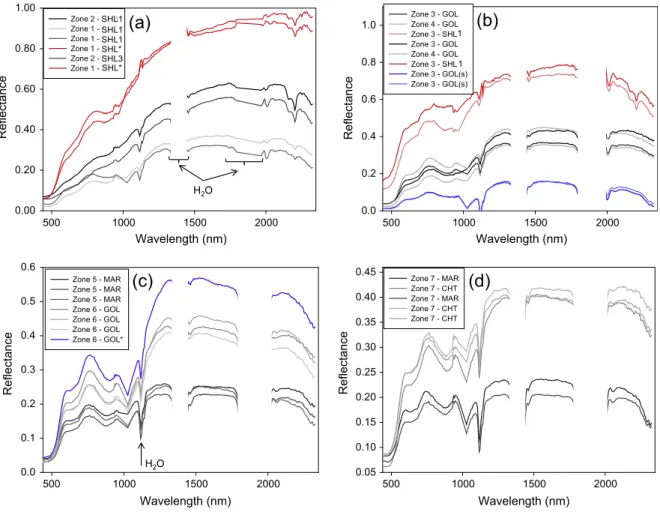
There were clear differences in the performance of methods between experiments. The GP-OAD and SAM performed well with quantitative and qualitative results showing that they performed better than SVMs and the GP-SE. The GP-SE, performed better than the SVM-based methods in Experiment 1. In Experiment 2, the GP-SE, however, failed to classify most rock types correctly. This is an interesting and significant finding. One possible reason for this might be that the training and the test data were acquired Wavelength (nm) 500 1000 1500 2000 Reflectance 0.00 0.20 0.40 0.60 0.80 1.00 Zone 2 - SHN Zone 1 - SHL Zone 1 - SHL Zone 1 - SHL* Zone 2 - SHN Zone 1 - SHL* Wavelength (nm) 500 1000 1500 2000 Reflectance 0.0 0.1 0.2 0.3 0.4 0.5 0.6 Zone 5 - MAR Zone 5 - MAR Zone 5 - MAR Zone 6 - GOL Zone 6 - GOL Zone 6 - GOL Zone 6 - GOL*
(a)
(c)
Wavelength (nm) 500 1000 1500 2000 Reflectance 0.05 0.10 0.15 0.20 0.25 0.30 0.35 0.40 0.45 Zone 7 - MAR Zone 7 - CHT Zone 7 - MAR Zone 7 - CHT Zone 7 - CHT(d)
Wavelength (nm) 500 1000 1500 2000 Reflectance 0.0 0.2 0.4 0.6 0.8 1.0 Zone 3 - GOL Zone 4 - GOL Zone 3 - SHL Zone 3 - GOL Zone 4 - GOL Zone 3 - SHL Zone 3 - GOL(s) Zone 3 - GOL(s)(b)
H2O H2O 1 1 SHL1 SHL1 SHL1 SHL3 SHL* SHL*Fig. 8.Spectra from different zones showing differences in brightness and curve shape for the same rock types as a consequence of illumination and surface coatings. (a) Spectra from Zones 1 and 2, red spectra are from areas covered in bright dust corresponding to the red dotted circle inFig. 3 and Fig. 7. (b) Spectra from Zones 3 and 4, red spectra are from an area covered in bright dust corresponding to the red circle in Zone 3. The blue spectra are from the shaded areas corresponding to the blue circles in Zone 3. (c) Spectra of GOL and MAR from Zones 5 and 6; the blue spectrum is from an area covered in bright dust corresponding to the blue dotted circle in Zone 6. (d) Spectra of MAR (black spectra corresponding to the black circle) and CHT (grey spectra corresponding to the grey circles) from Zone 7. Some CHT spectra exhibit very week clay absorptions near 2156 and 2202 nm. All spectra were smoothed for better visualisation. Note that spectra are not offset but exhibit large variations in brightness. (For interpretation of the references to colour in this figure legend, the reader is referred to the web version of this article.)
Table 4
Computational times required for the learning and inference (classification) stage for each classifier. Time required for inference is shown for both data sets (Experiments 1 and 2). Learning was done only once (for both data sets) as the training set was independent from each of the images. Times are shown in seconds. Times were measured using the MatlabÒ
functionality running on a WindowsÒ
7 PC equipped with an IntelÒ
Core™ i7-2630QM CPU and 12 GB RAM. All times are averages out of three measurements.
GP-OAD GP-SE SAM SVM-OAD SVM-SE
Learning 1.42 2.07 – 0.132 0.152
Inference (Exp1) 35.7 45.2 7.31 14.59 17.04
under different conditions of illumination (artificial vs natural) causing spectra in each dataset to have a different brightness. In field data, variations in brightness are also compounded by spatial variations in illumination of the mine face. Because the GP-SE uses a stationary (i.e. distance based) kernel, it is unable to accommodate these variations in brightness between the training and test data. A stationary measure is, theoretically, more affected by multiplicative variations than is SAM, the GP-OAD and the SVM-OAD. This was consistent with results which showed that angular metrics yielded the top three qualitative results for Experiment 2. The GP-SE outperformed the SVM-OAD in Experiment 1 because brightness variations were small due to data being acquired under artificial light. It is concluded from these findings that stationary kernels (used by the GP-SE and SVM-SE) will generally perform well where library and image spectra are acquired under similar or the same conditions of illumination. Care, therefore needs to be taken when applying stationary kernels for classification of imagery acquired in field conditions or where the albedo of rocks or minerals are different to those in the library spectra.
4.2. Consequences of calibration and illumination
Differences between library and image spectra may occur as a consequence of the different approaches used to calibrate them. Each library spectrum was calibrated using a calibration measurement obtained directly prior to acquisition of each target spectrum using artificial illumination. Pixel spectra from imagery of the mine face were affected by the intervening atmosphere, the effects of which can be seen in most spectra inFig. 8. Although the water absorption features around 1400 nm and 1900 nm are not observable in field imagery (they are largely obliterated by atmospheric water absorption), atmospheric absorption effects are still detectable in bands which are adjacent to their absorption maxima. These effects can introduce differences in spectral curve shape between library spectra and those of the mine face. Differences between library and image spectra are particularly problematic for shaded pixels because they are illuminated only by indirect light scattered back from clear skies or the mine wall. The wavelength-intensity distribution of indirect light is different from direct sunlight which illuminated the calibration panel. Indirect light would have proportionally more blue light caused by atmospheric scattering. Differences in curve shape between library spectra and those of the mine face resulting from these effects could explain the confusion between some rock types on the mine face e.g. MAR and GOL. Similar effects were reported by Murphy et al., 2012.
4.3. The GP-OAD’s advantages over SAM
Conventional implementations of SAM using a fixed threshold have been shown to perform sub-optimally because (i) optimal thresholds may vary depending on the particular library spectrum used and (ii) the optimal spectral angle of classification may vary among different rock types (Murphy et al., 2012). Consequently, in the present study, SAM was therefore used with the minimum angle criterion. This way, all spectra in the library were considered in the analysis, and no threshold had to be seta priori. This was also done because it allowed assigning classes in an analogous way to the other methods which used the maximum probability. SAM used the smallest angle, thus the largest similarity to assign class labels instead of the maximal probability. An inherent advantage of SAM is that it is relatively invariant to variations in brightness (van der Meer, 2006). This can be a disadvantage where the major discriminating factor between classes is their albedo, not curve shape, as in the case of MAR and GOL. In such cases, stochastic methods (e.g. GPs) may help by modelling the differences in the
classes better in a high dimensional space (e.g. the hyper-parameter space), particularly when the training set is large. The performance of the GP-OAD was similar to SAM, however, the GP-OAD’s greatest advantage is that it operates within a probabilistic framework. This provides the means to obtain a measure of uncertainty for every pixel in a classified image. The uncertainty obtained for each prediction using the GP-OAD may be useful when multiple classifications of the same target have to be fused into an optimal thematic map describing rock type or mineralogy. Using GP-OAD outputs can help to select the best classification automatically based on the smallest uncertainty or the highest probability (Schneider, 2013). Furthermore, the Bayesian framework may enable the integration of information from several sources such as other hyperspectral sensors and/or colour imagery. 4.4. Summary
Although zones were mapped by geologists to be of a specific rock type, zones were not entirely comprised of a single rock type as the target was a typical mine face with debris and dust present. The mineral composition of the mapped rock types in each zone may have been slightly different from the independent training set which was acquired from drill cores. Small-scale spatial variability in rock-type/mineralogy within each zone must also be assumed to cause within-zone spectral variability. The results obtained by SAM and the GP-OAD are good in most parts of the mine face given: (i) the training and test set were acquired different illumination (artificial versus natural light), (ii) rocks on the mine face were often coated in dust deposited as a part of the mining process, (iii) the effects due to shading and indirect illumination (e.g. from skylight and reflected light from the mine wall), (iv) a relatively small training set, and (v) the training and test set were independent from one another (i.e. drill cores versus whole rocks). All classifiers were used without manual tuning of their kernels or regularisation parameters, however, SVMs may be strongly affected by not tuning the SVM regularisation parameterC. This is a significant advantage of the GP-OAD over the SVM methods, especially in the context of autonomous mining and automated scene classification.
5. Conclusions
Results show that GPs can compete with the state-of-the art SVM classification approaches. In general, GPs:
(i) Provide class posterior probabilities.
(ii) Yield a variance estimate that can be exploited as a measure of confidence.
(iii) Operate in a Bayesian framework allowing the ability to: a. Integrate prior information in the classification process. b. Fuse data from several sensors or data of the same target
acquired at different times.
c. Select or weight features using automatic relevance determination kernels.
The main drawback of GPs is their high computational costs during inference. In this study no attempts were made to improve upon the computational speed, however, there are several methods to do this (e.g.Melkumyan and Ramos, 2009).
The experimental results obtained using the mine face imagery show that a non-stationary kernel (e.g. OAD kernel) or a kernel which is not based on the distance between two spectra is better suited for classification of hyperspectral data, particularly, when the training and test set were acquired independently and under different conditions of illumination. Although, the GP-OAD has
been applied to data acquired from a field-based platform, it may be applied to any hyperspectral image acquired from satellite or aircraft. Our choice of data acquired from a field-based platform allowed a more rigorous approach of validation. The results presented in this paper are therefore of direct relevance to all hyperspectral imagery, independent of the platform from which they were acquired.
Acknowledgements
This work has been supported by the Australian Centre for Field Robotics and the Rio Tinto Centre for Mine Automation. The authors would like to thank the anonymous reviewers whose comments improved this paper.
References
Alajlan, N., Bazi, Y., Alhichri, H., Othman, E., 2012. Robust classification of hyperspectral images based on the combination of supervised and unsupervised learning paradigms. In: Geoscience and Remote Sensing Symposium (IGARSS). 2012 IEEE International, pp. 1417–1420.
Bazi, Y., Melgani, F., 2006. Toward an optimal SVM classification system for hyperspectral remote sensing images. Geosci. Remote Sens., IEEE Trans. 44 (11), 3374–3385.
Bazi, Y., Melgani, F., 2008. Classification of hyperspectral remote sensing images using gaussian processes. In: Geoscience and Remote Sensing Symposium, 2008. IGARSS 2008. IEEE International, pp. II-1013–II-1016.
Bazi, Y., Melgani, F., 2010. Gaussian process approach to remote sensing image classification. Geosci. Remote Sens., IEEE Trans. 48 (1), 186–197.
Bishop, C.M., 2006. Pattern Recognition and Machine Learning (Information Science and Statistics). Springer-Verlag New York Inc., Secaucus, NJ, USA.
Brown, A.J., 2006. Spectral curve fitting for automatic hyperspectral data analysis. Geosci. Remote Sens., IEEE Trans. 44 (6), 1601–1608.
Chlingaryan, A., Melkumyan, A., Murphy, R.J., Schneider, S., 2013. Automated multi-class multi-classification of hyperspectral data using Gaussian Processes. In: Application of Computers and Operations Research in the Mineral Industry (APCOM). Porto Alegre, Brazil.
Clark, R.N., Gallagher, A.J., Swayze, G.A., 1990. Material absorption band depth mapping of imaging spectrometer data using a complete band shape least-squares fit with library reference spectra. In: Proceedings of the Second Airborne Visible/Infrared Imaging Spectrometer (AVIRIS) Workshop. JPL Publication, pp. 176–186.
Clark, R.N., Swayze, G.A., Livo, K.E., Kokaly, R.F., Sutley, S.J., Dalton, J.B., McDougal, R.R., Gent, C.A., 2003. Imaging spectroscopy: earth and planetary remote sensing with the USGS Tetracorder and expert systems. J. Geographical Res. 108. Clark, M.L., Roberts, D.A., Clark, D.B., 2005. Hyperspectral discrimination of tropical rain forest tree species at leaf to crown scales. Remote Sens. Environ. 96 (3–4), 375–398.
Congalton, R.G., Oderwald, R.G., Mead, R.A., 1983. Assessing landsat classification accuracy using discrete multivariate-analysis statistical techniques. Photogrammetric Eng. Remote Sens. 49 (12), 1671–1678.
Cudahy, T., Hewson, R., Caccetta, M., Roache, A., Whitbourn, L., Connor, P., Coward, D., Mason, P., Yang, K., Huntington, J., Quigley, M., 2009. Drill core logging of plagioclase feldspar composition and other minerals associated with Archean gold mineralization at Kambalda, Western Australia, using a bidirectional thermal infrared reflectance system Remote sensing and spectral geology. Rev. Econom. Geol. 16, 223–235.
Dehaan, R., Louis, J., Wilson, A., Hall, A., Rumbachs, R., 2007. Discrimination of blackberry (Rubus fruticosus sp. agg.) using hyperspectral imagery in Kosciuszko National Park, NSW, Australia. ISPRS J. Photogrammetry Remote Sens. 62 (1), 13–24.
Demarchi, L., Canters, F., Cariou, C., Licciardi, G., Chan, J.C.-W., 2014. Assessing the performance of two unsupervised dimensionality reduction techniques on hyperspectral APEX data for high resolution urban land-cover mapping. ISPRS J. Photogrammetry Remote Sens. 87, 166–179.
Doublier, M.P., Roache, T., Potel, S., 2010. Short-wavelength infrared spectroscopy: a new petrological tool in low-grade to very low-grade pelites. Geology 38 (11), 1031–1034.
Foody, G.M., Mathur, A., 2004. Toward intelligent training of supervised image classifications: directing training data acquisition for SVM classification. Remote Sens. Environ. 93 (1–2), 107–117.
Goetz, A.F.H., 2009. Three decades of hyperspectral remote sensing of the Earth: a personal view. Remote Sens. Environ. 113 (Supplement 1), S5.
Hecker, C., van der Meijde, M., van der Werff, H., van der Meer, F.D., 2008. Assessing the influence of reference spectra on synthetic SAM classification results. Geosci. Remote Sens., IEEE Trans. 46 (12), 4162–4172.
Hudson, W.D., Ramm, C.W., 1987. Correct formulation of the Kappa coefficient of agreement. Photogrammetric Eng. Remote Sens. 53, 421–422.
Hunt, G.R., Salisbury, J.W., 1970. Visible and near-infrared spectra of minerals and rocks; I, silicate minerals. Mod. Geol. 1 (7), 283–300.
Huntington, J., Mauger, A., Skirrow, R., Bastrakov, E., 2004. Automated mineralogical logging of core from the Emmie Bluff, iron oxide copper–gold prospect, south Australia. In: Pacrim 2004 Congress. Parkville, Victoria, pp. 223–230. Jiang, L., Zhu, B., Rao, X., Berney, G., Tao, Y., 2007. Discrimination of black walnut
shell and pulp in hyperspectral fluorescence imagery using Gaussian kernel function approach. J. Food Eng. 81 (1), 108–117.
Kruse, F.A., Lefkoff, A.B., Boardman, J.W., Heidebrecht, K.B., Shapiro, A.T., Barloon, P.J., Goetz, A.F.H., 1993. The spectral image processing system (SIPS)–interactive visualization and analysis of imaging spectrometer data. Remote Sens. Environ. 44 (2–3), 145.
Kruse, F.A., Bedell, R.L., Taranik, J.V., Peppin, W.A., Weatherbee, O., Calvin, W.M., 2011. Mapping alteration minerals at prospect, outcrop and drill core scales using imaging spectrometry. Int. J. Remote Sens. 33 (6), 1780–1798. Kurz, T., Buckley, S., Howell, J., Schneider, D., 2008. Geological outcrop modelling
and interpretation using ground based hyperspectral and laser scanning data fusion. ISPRS, Int. Arch. Photogrammetry, Remote Sens. Spatial Inform. Sci. XXXVII (8), 1229–1234.
Kurz, T.H., Buckley, S.J., Howell, J.A., Schneider, D., 2011. Integration of panoramic hyperspectral imaging with terrestrial lidar data. Photogram. Rec. 26 (134), 212–228.
Kurz, T.H., Buckley, S.J., Howell, J.A., 2013. Close-range hyperspectral imaging for geological field studies: workflow and methods. Int. J. Remote Sens. 34 (5), 1798–1822.
Li, J., Bioucas-Dias, J.M., Plaza, A., 2011. Hyperspectral image segmentation using a new bayesian approach with active learning. Geosci. Remote Sens., IEEE Trans. 49 (10), 3947–3960.
Lin, H.-T., Lin, C.-J., Weng, R.C., 2007. A note on Platt’s probabilistic outputs for support vector machines. Machine Learning 68 (3), 267–276.
Melkumyan, A., Nettleton, E., 2009. An observation angle dependent nonstationary covariance function for gaussian process regression. In: Lecture Notes in Computer Science. Springer, pp. 331–339.
Melkumyan, A., Ramos, F., 2009. A Sparse covariance function for exact gaussian process inference in large datasets. In: Twenty-First International Joint Conference on Artificial Intelligence (IJCAI-09). AAAI Press, Menlo Park, California.
Monteiro, S.T., Murphy, R.J., Ramos, F., Nieto, J., 2009. Applying boosting for hyperspectral classification of ore-bearing rocks. IEEE Int. Workshop Mach. Learn. Signal Process., 1–6.
Mountrakis, G., Im, J., Ogole, C., 2011. Support vector machines in remote sensing: a review. ISPRS J. Photogrammetry Remote Sens. 66 (3), 247–259.
Murphy, R.J., Monteiro, S.T., Schneider, S., 2012. Evaluating classification techniques for mapping vertical geology using field-based hyperspectral sensors. Geosci. Remote Sens., IEEE Trans. 50 (8), 3066–3080.
Murphy, R.J., Schneider, S., Monteiro, S.T., 2014a. Consistency of measurements of wavelength position from hyperspectral imagery: use of the ferric iron crystal field absorption at900 nm as an indicator of mineralogy. Geosci. Remote Sens., IEEE Trans. 52 (5), 2843–2857.
Murphy, R.J., Schneider, S., Monteiro, S.T., 2014b. Mapping layers of clay in a vertical geological surface using hyperspectral imagery: variability in parameters of SWIR absorption features under different conditions of illumination. Remote Sens. 6 (9), 9104–9129,http://www.mdpi.com/2072-4292/6/9/9104. Murphy, R.J., Schneider, S., Taylor, Z., Nieto, J., 2014. Mapping clay minerals in an
open-pit mine using hyperspectral imagery and automated feature extraction. In: First Vertical Geology Conference. Lausanne, Switzerland.
Nidamanuri, R.R., Zbell, B., 2011a. Normalized spectral similarity score (NS3) as an efficient spectral library searching method for hyperspectral image classification. Sel. Top. Appl. Earth Observations Remote Sens., IEEE J. 4 (1), 226–240. Nidamanuri, R.R., Zbell, B., 2011b. Use of field reflectance data for crop mapping
using airborne hyperspectral image. ISPRS J. Photogrammetry Remote Sens. 66 (5), 683–691.
Nocedal, J., Wright, S.J., 2006. Numerical Optimization, second ed. Springer-Verlag, New York, NY.
Olson, D.L., Delen, D., 2008. Advanced Data Mining Techniques. Springer-Verlag, Berlin, Germany.
Pasolli, L., Melgani, F., Blanzieri, E., 2010. Gaussian process regression for estimating chlorophyll concentration in subsurface waters from remote sensing data. Geosci. Remote Sens. Lett., IEEE 7 (3), 464–468.
Platt, J.C., 1999. Probabilistic outputs for support vector machines and comparisons to regularized likelihood methods. In: Advances in large margin classifiers. MIT Press, pp. 61–74.
Plaza, A., Benediktsson, J.A., Boardman, J.W., Brazile, J., Bruzzone, L., Camps-Valls, G., Chanussot, J., Fauvel, M., Gamba, P., Gualtieri, A., Marconcini, M., Tilton, J.C., Trianni, G., 2009. Recent advances in techniques for hyperspectral image processing. Remote Sens. Environ. 113 (Supplement 1), S110.
Ramanaidou, E., Wells, M., Belton, D., Verrall, M., Ryan, C., 2008. Mineralogical and microchemical methods for the characterization of high-grad banded iron formation – derived iron ore. Rev. Econom. Geol. 15, 129–156.
Rasmussen, C.E., Williams, C.K.I., 2006. Gaussian Process for Machine Learning. The MIT Press, Cambridge, Massachusetts.
Rencz, A.N., 1999. Remote sensing for the earth sciences – manual of remote sensing third. In: Rencz, A.N., Ryerson, R.A. (Eds.). John Wiley & Sons, New York. Rifkin, R., Klautau, A., 2004. In defense of one-vs-all classification. J. Mach. Learn.
Res. 5, 101–141.
Rodger, A., Laukamp, C., Haest, M., Cudahy, T., 2012. A simple quadratic method of absorption feature wavelength estimation in continuum removed spectra. Remote Sens. Environ. 118, 273–283.
Schneider, S., 2013. A probabilistic framework for classification and fusion of remotely sensed hyperspectral data. PhD-Thesis, University of Sydney, Australia. Schneider, S., Murphy, R.J., Monteiro, S., Nettleton, E.W., 2009. On the development
of a hyperspectral library for autonomous mining. In: Proceedings of Australasian Conference on Robotics and Automation (ACRA). Sydney, Australia. Schneider, S., Melkumyan, A., Murphy, R.J., Nettleton, E.W., 2010. Gaussian processes with OAD covariance function for hyperspectral data classification. In: Proceedings of IEEE International Conference on Tools with Artificial Intelligence. Arras, France.
Schneider, S., Murphy, R.J., Melkumyan, A., Nettleton, E., 2011. Classification of hyperspectral data of mine face geology using machine learning for autonomous open pit mining. In: Application of Computers and Operations Research in the Mineral Industry (APCOM). The Australasian Institute of Mining and Metallurgy (The AusIMM), Wollongong, Australia.
Schoelkopf, B., Burges, C., Smola, A., 1999. Support vector learning. In: Advances in Kernel Methods. MIT Press, Cambridge, MA, USA.
Shalev-Shwartz, S., Srebro, N., 2008. SVM optimization: inverse dependence on training set size. In: Proceedings of the 25th International Conference on Machine Learning. Helsinki, Finland.
Shrestha, D.P., Margate, D.E., van der Meer, F., Anh, H.V., 2005. Analysis and classification of hyperspectral data for mapping land degradation: an application in southern Spain. Int. J. Appl. Earth Obs. Geoinf. 7 (2), 85–96. Smola, A.J., Schölkopf, B., 2004. A tutorial on support vector regression. Statist.
Comput. 14 (3), 199–222.
Swayze, G.A., Clark, R.N., Goetz, A.F.H., Chrien, T.G., Gorelick, N.S., 2003. Effects of spectrometer band pass, sampling, and signal-to-noise ratio on spectral identification using the Tetracorder algorithm. J. Geographical Res. 108 (E9), 5105.
Swayze, G.A., Kokaly, R.F., Higgins, C.T., Clinkenbeard, J.P., Clark, R.N., Lowers, H.A., Sutley, S.J., 2009. Mapping potentially asbestos-bearing rocks using imaging spectroscopy. Geology 37 (8), 763–766.
Van der Meer, F., 2006. The effectiveness of spectral similarity measures for the analysis of hyperspectral imagery. Int. J. Appl. Earth Obs. Geoinf. 8 (1), 3–17. Van Rijsbergen, C.J., 1979. Information Retrieval. Butterworths, London. Vapnik, V.N., 1998. Statistical Learning Theory. Wiley, New York.
Vapnik, V.N., 2000. The Nature of Statistical Learning Theory. Springer-Verlag, New York, NY, USA.
Verrelst, J., Muñoz, J., Alonso, L., Delegido, J., Rivera, J.P., Camps-Valls, G., Moreno, J., 2012. Machine learning regression algorithms for biophysical parameter retrieval: opportunities for sentinel-2 and -3. Remote Sens. Environ. 118, 127–139.
Williams, C.K.I., Rasmussen, C.E., 1996. Gaussian processes for regression. In: Touretzky, D.S., Mozer, M.C., Hasselmo, M.E. (Eds.), Advances in Neural Information Processing Systems 8. The MIT Press, Cambridge, MA, USA, pp. 514–520.
Zaini, N., van der Meer, F., van der Werff, H., 2014. Determination of carbonate rock chemistry using laboratory-based hyperspectral imagery. Remote Sens. 6 (5), 4149–4172.