Robust Controller Design For Linear Systems With Nonlinear Distortions:
A Data-Driven Approach
Achille Nicoletti and Alireza Karimi
Abstract— The extensive use of frequency-domain tools for analyzing and controlling linear systems have become indis-pensable for the control systems engineer. However, due to the increased performance demands on today’s industrial systems, the effects of certain nonlinearities can no longer be neglected in control applications, and the use of these tools becomes problematic. In the current literature, however, frequency-domain methods exist where the underlying linear dynamics of a nonlinear system can be captured in an identification experiment; in this manner, the nonlinear system is replaced by a linear model with a noise source where a best linear approximation of the nonlinear system is obtained with an associated frequency-dependent uncertainty. This allows the use of robust control algorithms to ensure performance for the underlying linear system. In this paper, a data-drivenH∞ robust control strategy is presented which implements a convex optimization algorithm to ensure the performance and closed-loop stability of a linear system that is subject to nonlinear distortions. A case study is presented to illustrate how the proposed method can be used to design controllers for this class of systems.
I. INTRODUCTION
Frequency-domain techniques (such as the Bode, Nyquist, and Nichols plot) for analyzing and controlling linear sys-tems have become indispensable tools for the control syssys-tems engineer. To a certain degree, the effects of nonlineari-ties could be ignored because they did not impair system performance. However, due to the increased performance demands on today’s industrial systems, the effects of certain nonlinearities can impact the behavior of these systems. For many of today’s systems, the effects of nonlinearities can no longer be neglected (see [1] and [2]). Due to the extensive use of frequency-domain techniques for linear systems within the control systems community, and given the need for analyzing the effects of nonlinear systems, it is thus natural to extend the frequency-domain analysis and control schemes for linear systems where nonlinear distortions can occur. A comparative study of frequency-domain methods for nonlinear systems has recently been addressed in [3].
In addition to the problem of nonlinear effects in control systems, the problem of unmodelled dynamics in parameteric models is also prevalent in today’s industry. Systems are usually approximated with low-order models in order to reduce the complexity of a control design strategy. However, this approximation can lead to stability and performance degradations since these low-order models are subject to
A. Nicoletti is with the Technology Department, European Organi-zation for Nuclear Research (CERN), Switzerland. A. Karimi is with the Automatic Control Laboratory at Ecole Polytechnique F´ed´erale de Lausanne (EPFL), Switzerland. Corresponding author: Alireza Karimi:
model uncertainty. The data-driven control strategy mitigates the problems with model-based controller designs since the data-driven scheme avoids the problem of unmodeled dynamics associated with low-order parameteric models. A survey on the differences between the model-based control and data-driven control schemes has been addressed in [4] and [5].
Data-driven methods for controlling systems with non-linearities is a field which continues to spark the interests of many researchers. The authors in [6] present a model-free approach to design controllers that guarantee stability for a class of nonlinear discrete-time systems; in [7], this method is extended to the multiple-input-multiple-output (MIMO) nonlinear systems. A virtual reference feedback tuning (VRFT) method is proposed in [8] to design con-trollers for nonlinear plant models using a direct “one-shot” data-driven method. The authors in [9] build on the iterative learning control data-driven algorithm to design controllers for a class of nonlinear autoregressive exogenous models. A method for designing controllers in a data-driven setting for constrained linear systems is presented in [10]. The work in [11] extends on the concept of the VRFT method and implements a data-driven scheme to design linear parameter-varying (LPV) model-reference controllers.
Robust controller design methods belonging to the H∞
control framework for linear systems minimizes the H∞
norm of a weighted closed-loop sensitivity function. The objective of this paper is to combine the ideas presented in [12] and [13] and develop a data-driven controller design methodology that guarantees H∞ performance and
closed-loop stability for linear systems that are subject to nonlinear distortions. In [13], the frequency response function (FRF) of a nonlinear system is modeled as a best-linear-approximation (BLA) with an associated frequency dependent uncertainty. By performing a set of identification experiments on the nonlinear system, the dynamics of the underlying linear system are guaranteed to lie in the set of these uncertainties. In [12], a H∞ controller design scheme was formulated in which robust performance was obtained for a linear plant model that was subjected to frequency dependent uncertain-ties. Thus by considering the BLA of the nonlinear system as the nominal model, and by designing a controller which accounts for the frequency dependent uncertainties obtained from an identification experiment of the nonlinear system, the closed-loop stability and performance is be guaranteed for the underlying linear system.
This paper is organized as follows: In Section II, the class of controllers and nonlinearities are defined. Section III will
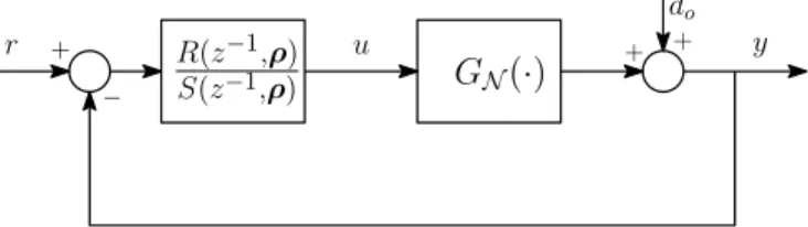
− + do R(z−1,ρ) S(z−1,ρ)
G
N(
·
)
+ + r u yFig. 1. Discrete-time controller structure.
address the control objectives and the conditions required for obtainingH∞performance and closed-loop stability for
the underlying linear model of a nonlinear system. A data-driven frequency-domain approach is implemented where the FRF measurement of a nonlinear system is modeled as a best linear approximation with an associated frequency dependent uncertainty. Section IV will demonstrate the effectiveness of the proposed method by designing fixed-structure controllers that ensure robust stability for the underlying linear system of a common motor control application. Finally the concluding remarks are given in Section V.
Notation: In order to avoid the risk of any confusion, the notation for the symbols employed in this paper will be defined here. R and R+ define the sets of all real numbers and real numbers greater than zero, respectively.
<{·} denotes the real part of the argument. (·)? denotes
the complex conjugate of the argument. The variables s
andz are the complex frequency variables used to represent continuous-time and discrete-time systems, respectively.
II. PRELIMINARIES
A. Class of Nonlinearities
The class of nonlinearities discussed in this work are now addressed with the following definition:
Definition 1. Class N of nonlinear systems.N is the set of nonlinear systems for which the following properties hold [13]:
• The influence of the initial conditions vanishes
asymp-totically.
• The steady state response to a periodic input is a peri-odic signal with the same period as the input. Nonlin-earities such as bifurcation, chaos, and sub harmonics are excluded; however, strongly nonlinear phenomena such as saturation and discontinuities are permitted.
• Only a point wise approximation of the output is ob-tained.
The nonlinear systems described byN include a class of nonlinearities known as the so called Wiener systems [14]. A nonlinear system which abides by the above definition will be denoted as GN(·)(i.e., GN(·)∈ N).
B. Class of Controllers
A fixed-order one-degree-of-freedom polynomial control structure is considered. The general structure of this control system is shown in Fig. 1. The functions R(z−1, ρ) and
Nonlinear System Linear System + U(e−jω) U(e−jω) Y(e−jω) YL(e−jω) YS(e−jω) Y(e−jω)
Fig. 2. Representation of a nonlinear system by a linear system for a certain class of inputs.
S(z−1, ρ)each represent linearly parameterized polynomials inz−1, i.e.,
R(z−1) =r0+r1z−1+· · ·+rnrz
−nr (1)
S(z−1) = 1 +s1z−1+· · ·+snsz
−ns (2)
whereri and si are the controller parameters and {nr, ns}
are the orders of the polynomialsRandS, respectively. The vector of controller parametersρis defined as:
ρ>= [r0, r1, . . . , rnr, s1, s2, . . . , sns] (3)
whereρ∈Rn withn=nr+ns+ 1.
III. ROBUSTDESIGN WITHNONLINEARDISTORTIONS
In this section, a data-driven method is implemented such that the underlying linear dynamics of a system GN(·)
are captured in the FRF during an experiment (where the underlying linear system can be fully characterized as a best-linear-approximation of the measured FRF with an associated uncertainty). A convex optimization problem can then be formulated by minimizing the norm of a weighted sensitivity function to guarantee the closed-loop stability and performance of the linear system that is subject to nonlinear distortions.
A. Quantification of Nonlinear Distortions
Suppose that the signals uand y are measurable. Let us denote the frequency spectrum of the signals u and y as
U(e−jω) andY(e−jω), respectively. According to [13], for a certain class of reference signals and nonlinear systems, the FRF obtained during an experiment with a nonlinear plant can be described by a linear system plus an error term
YS(e−jω)(see Fig. 2). The class of nonlinear systems that can be considered with this approach are those inN.
The idea asserted in [13] is to perform multiple experi-ments with full or random phase multisines as the reference input. Averaging of the FRFs over the consecutive periods quantifies the noise level. Averaging of these mean FRFs over multiple experiments quantifies the level of the stochastic nonlinear distortions (with the sum of the remaining noise level).
Definition 2. Random Phase Multisine: u(t) is a random phase multisine if u(t) = K/2−1 X k=−K/2+1 Ukej2πfskt/K (4)
where Uk =U?
−k =|Uk|ejφk, fs is the clock frequency of
the waveform generator,K is the number of samples in the signal period, and the phases φk are a realization of an
independent distributed random process in[0,2π)where the expected value of ejφk is equal to zero.
1) Stable Plant: Let us first consider the case when the plant model is stable; for a given known input signal, an open-loop experiment can be performed to obtain the FRF BLA and the variance. Let us defineG[q,p](e−jω)as the FRF estimate of GN(·)for the p-th period of a q-th experiment
(with P denoting the total number of periods in each experiment andQbeing the total number of experiments):
G[q,p](e−jω) = Y
[q,p](e−jω) U[q](e−jω)
=G(e−jω) +G[Sq](e−jω) +EG[q,p](e−jω)
(5)
where G is the FRF BLA, G[Sq] = YS[q]/U[q] (i.e., the stochastic nonlinear contributions) and E[Gq,p] are the errors due to the output noise. The sample mean and the sample variance of the FRF estimates overP periods are determined as follows: G[q](e−jωk) = 1 P P X p=1 G[q,p](e−jωk) σn2[q](k) = 1 P(P−1) P X p=1 G [q,p](e−jωk)−G[q](e−jωk) 2 (6) whereσ2[nq] is the sample noise variance of the sample mean G[q]. The BLA of the plant G with the associated sample total varianceσ2
Gcan then be determined with the following
relations [13]: G(e−jωk) = 1 Q Q X q=1 G[q](e−jωk) σ2G(k) = 1 Q(Q−1) Q X q=1 G [q](e−jωk)−G(e−jωk) 2 (7)
2) Unstable Plant: Let us now consider the case when the plant model is unstable; in this case, an open-loop experiment cannot be performed to obtain the FRFs. A stabilizing controller would first need to be implemented in order to stabilize the closed-loop system (i.e., all outputs remain bounded for a bounded reference signal). Now, suppose that the signalris measurable where the frequency spectrum ofr
is denoted asR(e−jω). Additionally, let us defineN(e−jω)
as the FRF BLA between the signalsrtoyandM(e−jω)as the FRF BLA between the signalsrtou. Since the nonlinear system is described by a linear system plus an error term
YS(e−jω), then it is evident that the FRF BLA of the plant model G(e−jω) = N(e−jω)M−1(e−jω). This is known as acoprime factorizationof the FRF GwhereN andM are coprime functions which are analytic outside the unit circle [15].
According to [13], the sample means and total (co)variances can be determined as follows:
Y(e−jωk) = 1 Q Q X q=1 Y[q](e−jωk) σY2(k) = 1 Q(Q−1) Q X q=1 Y[q](e−jωk)− Y(e−jωk) 2 σYR2 (k) = 1 Q(Q−1) Q X q=1 Y[q](e−jωk)− Y(e−jωk)· R[q](e−jωk)− R(e−jωk)? σU R2 (k) = 1 Q(Q−1) Q X q=1 U[q](e−jωk)− U(e−jωk)· R[q](e−jωk)− R(e−jωk)? (8) where the FRFs and variances for the signals u (i.e.,
U(e−jωk)andσ2
U(k)) andr(i.e.,R(e−jωk)andσR2(k)) are
are computed in the same manner asY(e−jωk)andσ2 Y(k),
respectively. For notation purposes, the dependency ine−jω
will be omitted, and will only be reiterated when deemed necessary. Finally, the FRF of the BLA for each coprime can then be obtained asN=YR−1andM =U R−1where the associated total variance for each coprime is calculated as follows: σN2 =N 2 σ2Y |Y|2 + σ2 R |R|2 −2< σ2 YR YR? σ2M =M 2 σU2 |U |2 + σR2 |R|2 −2< σ2 U R U R? (9)
Remark. Note that in [13], the FRF estimate ofG(and the associated uncertainty) can be obtained from the signalsu andydirectly. However, the coprime formulation was needed in this paper in order to apply the proposed controller design schemes (which are asserted in Section III-B).
Suppose that the uncertainty associated with a given FRF is described by an additive uncertainty:
ˆ N(e−jω) =N(e−jω) +|Wn(e−jω)|δnejθn ˆ M(e−jω) =M(e−jω) +|Wm(e−jω)|δmejθm (10) where|δn| ≤1,|δm| ≤1; {θn, θm} ∈[0,2π];Wn andWm
are the uncertainty weighting filters which can be determined from the covariance of the estimates for a given confidence interval. Given the frequency spectrums ofY,U andR, the estimates of the real and the imaginary part ofN(e−jω)and
M(e−jω) can be formulated; these estimates are asymptot-ically uncorrelated and normally distributed [16]. For any givenω, the additive uncertainty forNˆ can be described in the complex plane with a disk centered atN having a radius of |Wn| (when the worst case scenario is considered with δn = 1). A similar representation can be made withMˆ. The
uncertainty is characterized by the Rayleigh distribution and can be determined for any probability level. For example, if it is desired to construct an uncertainty disk such that the true frequency response lies within the disk with a probability
level of0.95, then the radius of this disk(s) will be |Wn(e−jω)|= q 5.99σ2 N ; |Wm(e −jω)|=q5.99σ2 M (11)
B. Robust Controller Design
In the general H∞ control problem for linear systems, the objective is to minimize an upper bound γ to find the controller parameter vector ρsuch that
sup ω∈Ω
|Wl(e−jω)Sl(e−jω,ρ)|< γ (12) whereΩ := [−π/Ts, π/Ts] (withTs[s] being the sampling
time of the process), γ ∈ R+, Sl is the l-th sensitivity
function of interest, andWlis the FRF of a stable weighting
filter such thatWlSl(ρ)has a bounded infinity norm. In [12], the linear plant model was represented asG=N M−1where N andM were coprimes functions that were both stable and proper. Therefore, a general construction of the sensitivity function can be expressed as Sl(ρ) = ∆l(ρ)/ψ(ρ), where
∆l(ρ)is a linear function ofR(ρ) orS(ρ)and
ψ(ρ) =N R(ρ) +M S(ρ)
The subscript l ∈ {1,2,3,4} denotes the l-th sensitivity of interest. As an example, the sensitivity function S1 from r to r−y is ∆1(ρ)/ψ(ρ) where ∆1(ρ) = M S(ρ). Given this construction, the condition in (12) can be expressed as follows:
γ−1|Wl∆l(ρ)|<|ψ(ρ)|, ∀ω∈Ω (13)
For any given frequency inΩ, the condition in (13) represents a circle in the complex plane which does not include the ori-gin and is centered atψ(ρ)with a radius ofγ−1|W
l∆l(ρ)|.
In [12], it is shown that there exists a complex function
f(e−jω) which can rotate this circle such that it lies on the right-hand side of the imaginary axis. This geometrical construction is used to formulate a necessary and sufficient condition for (12), which is recalled in the following Theo-rem:
Theorem 1. Given the frequency response function G(e−jω) = N(e−jω)M−1(e−jω) and the frequency
re-sponse of a weighting filter Wl(e−jω), then the following statements are equivalent:
(a) There exists a controller that stabilizesGand
sup ω∈Ω
|WlSl(ρ)|< γ (14)
(b)There exists a controller such that
<{ψ(ρ)}> γ−1|Wl∆l(ρ)| ∀ω∈Ω (15)
Proof :The proof is given in [12].
Given the additive uncertainty in (10), a desired perfor-mance condition kWlSlk∞ < γ can be satisfied for all
models in the uncertain set (10) if kWlSlkˆ ∞ < γ, where ˆ
Sl= ˆ∆l/ψˆ(ρ)andψˆ(ρ) = ˆN R(ρ) + ˆM S(ρ). For example,
consider the nominal performance conditionkW1Sˆ1k∞< γ
with ∆ˆ1(ρ) = ˆM S(ρ); as a worst case consideration, δm
and δn can be selected to be equal to one in (10) (which
ensures that the uncertainty in the entire disk is taken into account). By substituting the expressions in (10) into this condition, the following constraint can be devised:
W1S(ρ) M+|Wm|ejθm < γ ψ(ρ) + Γ(ρ, θn, θm) ∀ω∈Ω,∀{θn, θm} ∈[0,2π] (16) whereψ(ρ) =N R(ρ) +M S(ρ)and Γ(ρ, θn, θm) =S(ρ)|Wm|ejθm+R(ρ)|Wn|ejθn
For a given{ω, θn, θm}, (16) represents a circle centered at
ψ(ρ) + Γ(ρ, θn, θm)with a radius of
xp(ρ, θm) =γ−1W1S(ρ)
M+|Wm|ejθm
(17)
that does not include the origin.
Given the results from Theorem 1, a necessary and suffi-cient condition for (16) can be formulated as follows:
xp(ρ, θm)<<
ψ(ρ) + Γ(ρ, θn, θm)
∀ω∈Ω,∀{θm, θn} ∈[0,2π]
(18)
By gridding in ω,θm and θn, (18) then becomes a convex
constraint (with respect to ρ); however, gridding in all of these variables can be computationally expensive. Therefore, a sufficient condition for (16) can be devised as follows:
sup ω∈Ω |W1S(ρ)| |M|+|Wm| |ψ(ρ)| −Γs(ρ) < γ (19)
whereΓs(ρ) =|S(ρ)Wm|+|R(ρ)Wn|.With this condition,
the dependency inθmandθnhas been removed, and gridding
in only one variable (i.e., ω) is required. The condition in (19) can be represented as a disk in the complex plane which is centered atψ(ρ)and has radius
xr(ρ) =γ−1|W1S(ρ)| h
|M|+|Wm|
i
+ Γs(ρ) (20)
Therefore, a set of convex constraints (with respect toρ) can be devised with the following condition:
xr(ρ)<<{ψ(ρ)}, ∀ω∈Ω (21) Note that (19) introduces some conservatism; however, this conservatism can always be reduced by imposing (18) (at the price of a larger computation time).
C. Convex Optimization via Semi-Definite Programming With the constraints developed in the previous section, an optimization problem can be formulated to guarantee
H∞performance and closed-loop stability for the underlying linear system. For nominal performance (i.e., kW1Sˆ1k∞ < γ), the following optimization problem is considered:
minimize γ,ρ γ subject to: xr(ρ)<< ψ(ρ) ∀ω∈Ω (22)
This optimization problem is quasi-convex; to solve such a problem, a bisection algorithm can be realized where
an iterative approach is implemented in order to obtain an asymptotically convergent solution for γ. The above optimization problem also possesses an infinite number of constraints; thus a semi-definite programming (SDP) algo-rithm can be implemented where a predefined frequency grid is used in order to solve a finite number of constraints. This frequency grid can be predefined in a variety of manners (see [17], [18]).
IV. CASESTUDY
In this case study, a DC motor with a typical nonlinearity encountered in practice is considered. The model of the brushless DC motor is taken from [19]:
G(z) = 0.0143z+ 0.0142
(z−1)(z−0.9725) (23)
where the sampling time of the process is given as Ts = 2.048ms. A typical nonlinearity that is encountered with motor applications is the dead-zone nonlinearity (see [20], [21]). This nonlinearity would occur at the input of the plant, and can be expressed as follows:
u= 0, for −d≤un≤d m(un−d), for un> d m(un+d), for un<−d (24)
where un is the input to the nonlinearity, m is the slope
of the line, and d∈]0,∞[ is the value of un at which the
discontinuity occurs.
The objective of this case study will be to demonstrate the effectiveness of the proposed robust design method by applying a random-phase multisine signal that excites the dead-zone nonlinearity; the FRF obtained from this identifi-cation will then be used to model a BLA with an associated uncertainty and design a robust controller that minimizes
kW1Sˆ1k∞. For simplicity, the values of the nonlinearity are selected as m= 1 andd = 0.1 for this case study. It will also be desired to investigate the response of a controller when the uncertainties in the design are neglected and the FRF of the coprimes are obtained from a given time-domain experiment.
For this case study, the closed-loop system is stabilized when a proportional controller is implemented with a unity-feedback structure (with the value of the controller equal to
0.15). The closed-loop system was excited with a periodic random phase multisine (with an amplitude range of ±50);
10 experiments were performed where the system was ex-cited with15periods of this signal where the period length was 2000 samples and each period contains 500 sinusoids with random phases.
For comparative purposes, it was desired to compare the design scheme when the uncertainties of the proposed method were neglected and the nominal FRF was obtained directly from the data. The FRF BLAs with the associated uncertainties for Nˆ andMˆ are shown in Fig. 3 and Fig. 4, respectively. The radii of the uncertainty circles for each coprime were computed using (11). It can be observed that at some frequencies, the FRF of the coprimes for a given
Fig. 3. N (dashed-blue line) with the associated uncertainties at each frequency (black circles). The FRF obtained between r(t) to y(t)for a given experiment with no uncertainties (dashed-red line).
Fig. 4. M (dashed-blue line) with the associated uncertainties at each frequency (black circles). The FRF obtained betweenr(t)to u(t)for a given experiment with no uncertainties (dashed-red line).
experiment are not included in the uncertainty disks. With the BLA and the uncertainty for the coprimes, a controller was computed in order to obtain H∞ performance for the
underlying linear system.
1) Weighting filter selection: The weighting filters Wn
andWm for the uncertainties in Nˆ andMˆ were calculated
using (11). The weighting filter W1 was selected based on a desired closed-loop reference model. For the underlying linear system, it is know that S1 +S2 = 1, where S2 is the complementary sensitivity function (i.e., the closed-loop transfer function). A simple first-order closed-loop reference model was selected as the desired complementary function
Sd
2(z) = (1−a)(z−a)−1
wherea=e−ωdTs and ω
d[rad/s] is the desired bandwidth.
For this case study, the desired bandwidth was selected as
ωd = 100π. Thus W1 was formulated as [1− S2d(z)]−1.
Note that the controller was prefixed with an integrator, and
kW1Sˆ1k∞ remains bounded∀ω.
2) Simulation Results: The problem in (22) was solved in SDP form with the 500 frequency points obtained from the random-phase multi-sine experiments and with a 5th
order controller. To invoke integral action, the controller was prefixed with an integrator. Two design schemes were considered:
• A design in which the FRF BLA with the associated
frequency dependent uncertainties were considered.
Time [s]
Amplitude
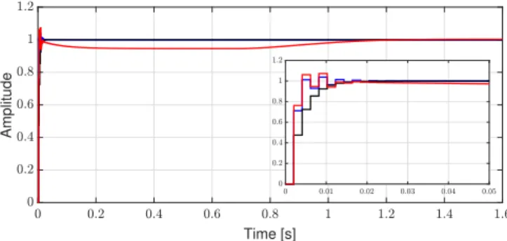
Fig. 5. Step response of the nonlinear system. The desired closed-loop response (black line); the response with the proposed method (including uncertainties in design) (blue line); the response with no uncertainties considered (red line).
|Wn| = |Wm| = 0) and the FRF of the coprimes is obtained from a given experiment.
The optimal solution to the proposed convex problem was computed asγ?= 1.252 (using a tolerance of 10−3 for the bisection algorithm) with an optimization time of 108.2s. This optimization time was calculated based on a computer having the following hardware specifications: Intel-Core i7, 3.4 GHz CPU, 8GB RAM. The optimization algorithms were run usingMATLABversion (R2017a) on a Windows 7 plat-form (64-bit). The closed-loop step response of the nonlinear system is shown in Fig. 5; it can be observed that when the frequency-dependent uncertainties are considered in the design, good performance and stability is achieved. When the uncertainties are neglected in the design, the settling time is significantly larger. This is caused by the modeling error from the closed-loop experiment (which can be seen in figures 3 and 4 where the FRF lies outside the uncertainty disks at various frequency points). Thus with the proposed method, the performance and stability of the underlying linear system can be guaranteed by considering the fre-quency dependent uncertainties obtained from the random-phase multi-sine identification experiments performed on a nonlinear system.
V. CONCLUSION
In this paper, a data-driven method has been proposed for designing fixed-structure controllers for linear systems with nonlinear distortions. In this method, a robust design was implemented where the FRF obtained from an identification experiment of the nonlinear system was modeled as a BLA with an associated uncertainty (to capture the dynamics of the underlying linear system). A convex optimization algorithm was then devised to guarantee H∞ performance
and stability for this underlying linear system. The case study has confirmed the effectiveness of the proposed method by designing a a controller for a typical system where the dead-zone nonlinearity occurs frequently in practice. For future work, it will be desired to extend the proposed robust control design methodology for MIMO systems.
REFERENCES
[1] Y. Meyer and G. Cumunel, “Active vibration isolation with a MEMS device: Effects of nonlinearities on control efficiency,”Smart Materials and Structures, vol. 24, no. 8, p. 085004, 2015. [Online]. Available: http://stacks.iop.org/0964-1726/24/i=8/a=085004
[2] E. d. A. Barboza, M. J. da Silva, L. D. Coelho, J. F. Martins-Filho, C. J. A. Bastos-Filho, U. C. de Moura, and J. R. F. de Oliveira, “Impact of nonlinear effects on the performance of 120 gb/s 64 qam optical system using adaptive control of cascade of amplifiers,” in2015 SBMO/IEEE MTT-S International Microwave and Optoelectronics Conference (IMOC), Nov 2015, pp. 1–5.
[3] D. Rijlaarsdam, P. Nuij, J. Schoukens, and M. Steinbuch, “A comparative overview of frequency domain methods for nonlinear systems,” Mechatronics, vol. 42, no. Sup-plement C, pp. 11 – 24, 2017. [Online]. Available: http://www.sciencedirect.com/science/article/pii/S0957415816301568 [4] Z.-S. Hou and Z. Wang, “From model-based control to data-driven
control: Survey, classification and perspective,”Information Sciences, vol. 235, pp. 3–35, 2013.
[5] S. Formentin, K. Van Heusden, and A. Karimi, “A comparison of model-based and data-driven controller tuning,” Int. Journal of Adaptive Control and Signal Processing, 2013.
[6] Z. Hou and S. Jin, “A novel data-driven control approach for a class of discrete-time nonlinear systems,” IEEE Transactions on Control Systems Technology, vol. 19, no. 6, pp. 1549–1558, 2011.
[7] ——, “Data-driven model-free adaptive control for a class of MIMO nonlinear discrete-time systems,”IEEE Transactions on Neural Net-works, vol. 22, no. 12, pp. 2173–2188, 2011.
[8] M. C. Campi and S. M. Savaresi, “Direct nonlinear control design: The virtual reference feedback tuning (VRFT) approach,”IEEE Trans. on Automatic Control, vol. 51, no. 1, pp. 14–27, 2006.
[9] M. B. Radac, R. E. Precup, E. M. Petriu, and S. Preitl, “Iterative data-driven tuning of controllers for nonlinear systems with constraints,”
IEEE Transactions on Industrial Electronics, vol. 61, no. 11, pp. 6360– 6368, Nov 2014.
[10] D. Piga, S. Formentin, and A. Bemporad, “Direct data-driven con-trol of constrained systems,”IEEE Transactions on Control Systems Technology, vol. PP, no. 99, pp. 1–8, 2017.
[11] S. Formentin, D. Piga, R. T´oth, and S. M. Savaresi, “Direct learning of lpv controllers from data,”Automatica, vol. 65, pp. 98–110, 2016. [12] A. Karimi, A. Nicoletti, and Y. Zhu, “RobustH∞ controller design
using frequency-domain data via convex optimization,”International Journal of Robust and Nonlinear Control, 2016. [Online]. Available: http://dx.doi.org/10.1002/rnc.3594
[13] R. Pintelon and J. Schoukens, System identification: a frequency domain approach. John Wiley & Sons, 2012.
[14] M. Schetzen, The Volterra and Wiener theories of nonlinear systems. Wiley, Apr. 1980. [Online]. Avail-able: http://www.amazon.com/exec/obidos/redirect?tag=citeulike07-20&path=ASIN/0471044555
[15] K. Zhou and J. C. Doyle,Essentials of robust control. N.Y.: Prentice-Hall, 1998.
[16] L. Ljung,System Identification - Theory for the User, 2nd ed. NJ, USA: Prentice Hall, 1999.
[17] P. Seiler, B. Vanek, J. Bokor, and G. J. Balas, “Robust H∞ filter
design using frequency gridding,” in American Control Conference (ACC), 2011. IEEE, 2011, pp. 1801–1806.
[18] G. Galdos, A. Karimi, and R. Longchamp, “H∞controller design for
spectral MIMO models by convex optimization,”Journal of Process Control, vol. 20, no. 10, pp. 1175 – 1182, 2010.
[19] W. Zhang, M. Tomizuka, P. Wu, Y. H. Wei, Q. Leng, S. Han, and A. K. Mok, “A double disturbance observer design for compensation of unknown time delay in a wireless motion control system,”IEEE Transactions on Control Systems Technology, vol. PP, no. 99, pp. 1–9, 2017.
[20] W. Shi, H. Zhao, J. Ma, and Y. Yao, “Dead zone compensation of ultrasonic motor using adaptive dither,” IEEE Transactions on Industrial Electronics, vol. PP, no. 99, pp. 1–1, 2017.
[21] C. Hu, B. Yao, and Q. Wang, “Adaptive robust precision motion control of systems with unknown input dead-zones: A case study with comparative experiments,”IEEE Transactions on Industrial Electron-ics, vol. 58, no. 6, pp. 2454–2464, June 2011.