Robust Subsampling
∗Lorenzo Camponovo
University of LuganoOlivier Scaillet
University of Geneva and Swiss Finance Institute
Fabio Trojani
University of Lugano and Swiss Finance Institute First Version: November 2006. This Version: July 2011.
∗We thank the editor (Takeshi Amemiya), the associate editor and two anonymous referees for
useful comments. The authors acknowledge the financial support of the Swiss National Science Foun-dation (NCCR FINRISK and grants 101312-103781/1, 100012-105745/1, and PDFM1-114533). We thank participants at the ESEM 2006 in Vienna, the 2007 Meeting of the Swiss Society of Economics and Statistics in St. Gallen, the 2007 International Workshop on Computational and Financial Econo-metrics in Geneva, and the 2007 International Conference on Robust Statistics in Buenos Aires, for helpful comments. Part of this research was done when the first author was visiting Yale University as a post doctoral researcher. Correspondence address: Fabio Trojani, Faculty of Economics, University of Lugano, Via Buffi 13, CH-6900 Lugano, e-mail: [email protected].
Abstract
We characterize the robustness of subsampling procedures by deriving a formula for the breakdown point of subsampling quantiles. This breakdown point can be very low for moderate subsampling block sizes, which implies the fragility of subsampling procedures, even when they are applied to robust statistics. This instability arises also for data driven block size selection procedures minimizing the minimum confidence interval volatility in-dex, but can be mitigated if a more robust calibration method can be applied instead. To overcome these robustness problems, we introduce a consistent robust subsampling procedure for M-estimators and derive explicit subsampling quantile breakdown point characterizations for MM-estimators in the linear regression model. Monte Carlo simula-tions in two settings where the bootstrap fails show the accuracy and robustness of the robust subsampling relative to the subsampling.
Keywords: Subsampling, bootstrap, breakdown point, robustness.
JEL:C12, C13, C15.
1
Introduction
Resampling methods are powerful tools in modern statistics and econometrics; bootstrap pro-cedures (see, e.g., Hall, 1992, Efron and Tibshirani, 1993, and Hall and Horowitz, 1996) and subsampling procedures (Politis and Romano, 1992, 1994) have widespread applicability, and are useful for a wide variety of inference problems in many fields. The bootstrap has been the object of a huge research in statistics and econometrics, since its introduction by Efron (1979). Subsampling procedures are more recent, but have gained rapidly considerable attention. The simpler consistency conditions and the wider applicability in some cases (see, e.g., Andrews, 2000, and Bickel et al., 1997, for some famous examples) make subsampling a useful and valid alternative to the bootstrap. Some examples of recent applications of subsampling proce-dures include: Chernozhukov and Fernandez-Val (2005), who analyze subsampling inference of quantile regression processes; Gonzalo and Wolf (2005), who study subsampling inference in threshold autoregressive models; Linton, Maasoumi and Whang (2005), who develop a sub-sampling testing procedure for stochastic dominance; Hong and Scaillet (2006), who propose a fast subsampling method for nonlinear dynamic models; Lee and Pun (2006), who investigate subsampling in nonstandard M-Estimation with nuisance parameters.
As emphasized, for instance, by Bickel et al. (1997), a key issue in the application of subsampling methods is the selection of an adequate subsampling block size m among the n
data points, because subsampling accuracy can highly depend on this parameter. Hall and Yao (2003) highlight this problem for GARCH settings with asymmetric heavy-tailed errors. Cowell and Flachaire (2007) and Davidson and Flachaire (2007) observe a similar problem when resampling inequality and poverty measures. Our goal in this paper is to study the robustness of subsampling methods in relation to the choice of the subsampling block size.
The need for robust statistical procedures has been stressed by many authors and is now widely recognized; see, e.g., Huber (1981), Hampel, Ronchetti, Rousseeuw and Stahel (1986), Heritier and Ronchetti (1994), Sakata and White (1998), Ronchetti and Trojani (2001), Ortelli and Trojani (2005), Mancini, Ronchetti and Trojani (2005), and La Vecchia and Trojani (2010). A natural question is this context is whether standard subsampling methods applied to robust
statistics already imply a robust subsampling inference. The answer is no and motivates our interest for robust versions of the subsampling approach.
The following example, inspired by Singh (1998) in the bootstrap setting, illustrates the intuition for the failing robustness of the standard subsampling, even when applied to a robust statistic. Consider the 10% trimmed mean Tn := T(X1, . . . , Xn; 0.1) (i.e., 5% trimming each
side) on a random sample (X1, . . . , Xn) of size n = 200. If there are 8 outliers in the upper
tail, that is, the order statistics {X(193), ...X(200)}are extraordinarily large,Tn stays unaffected
due to the trimming. Now suppose a subsample (X1∗, . . . , Xm∗) of size m= 20 is drawn without replacement from this sample. One outlier out of {X(193), ...X(200)} could appear, two outliers could appear, or, in the most extreme case, the whole set of outliers could appear in the subsample. Consider the subsampling distribution of the trimmed mean. If one outlier appears, the subsampling statisticTn,m∗ :=T(X1∗, . . . , Xm∗; 0.1) is free ot it. If at least two outliers appear, it is not. The chances for the event thatTn,m∗ is free of a single outlier isp0 =P[X(200,20, .04) ≤ 1], which is about 80%, where X(n, m, p) denotes an hypergeometrically distributed random variable, with parameters n, np, and m. This means that if the order statistics diverge to infinity, 100(1−p0)% of all subsampling statistics diverge to infinity as well. In other words, the subsampling quantile Q∗t,n,m of Tn,m∗ , where t ranges from 0 to 1, will go to infinity for all probability levels t > p0 ' 80%. This illustrates that the subsampling distribution of the trimmed mean is not immune from the breakdown of its upper quantile when t > p0, and is thus not robust to the presence of outliers in the original sample. This simple example also indicates that the subsampling tends to be more fragile than its bootstrap counterpart. The chances for the event that the bootstrap statistic Tn∗ := T(X1∗, . . . , Xn∗; 0.1) computed on a bootstrap sample (X1∗, . . . , Xn∗) of size n= 200 is free of 10 outliers isP[B(200, .04) ≤10] =p0, which is about 82%, whereB(n, p) denotes a binomial random variable, with parametersnand
p. Moreover, the above arguments also show that lower subsampling block sizes strengthen the subsampling robustness problem. For example, it is easy to see that in the above setting a block size m = 10 implies a chance of only 66% for the event that Tn,m∗ does not depend on a single outlier.
subsam-pling instability. We derive a formula for the breakdown point of subsamsubsam-pling quantiles, i.e., we compute the smallest fraction of outliers in the original sample such that the subsampling quantile diverges to infinity. When this occurs, inference based on subsampling distributions becomes meaningless. Indeed, critical values of subsampling-based tests diverge to infinity, and confidence intervals computed using subsampling distributions have an infinite length. It turns out that in this case both the size and the power of subsampling-based tests collapse to zero or one. Consequently, the quantile breakdown point is an important global robustness tool for describing up to which fraction of contaminations the subsampling distribution still provides some reliable information. We show that the subsampling quantile breakdown point is increas-ing in the subsamplincreas-ing block size, the sample size, and the breakdown point of the statistic used. Concrete computations show that moderate block sizes typically chosen in applications can imply very unstable subsampling quantiles even when exploiting robust statistics. This instability is larger than the one observed for standard bootstrap quantiles; see, e.g., Singh (1998), and Salibian-Barrera and Zamar (2002). As shown in Section 2.2, it also arises for data driven block size selection procedures based on the minimum confidence interval volatility (MCIV) index, but can be mitigated by a more robust calibration approach (Romano and Wolf, 2001). To overcome these robustness problems, we introduce a robust subsampling method for M-estimators in Section 2.3. We further analyze in detail the properties of the robust subsam-pling for MM-estimates in the linear regression setting, by computing its breakdown point and by proving its consistency in Section 2.4. Monte Carlo simulations and sensitivity analysis are presented in Section 3, for two settings where the bootstrap fails. In the first example, we study the inference about the squared mean of a random variable. In the second example, we study a linear regression model with a parameter of interest near a boundary. Andrews and Guggen-berger (2009a,b, 2010a,b) show that subsampling methods may imply a distorted asymptotic size, when applied to statistics with a discontinuous asymptotic distribution in some model parameter. They propose hybrid subsampling methods to overcome the problem. We borrow from their approach to compute confidence intervals for the relevant parameter using hybrid robust subsampling procedures. Section 4 gathers concluding remarks.
2
Subsampling Breakdown Point and Robust
Subsam-pling
Let (X1, . . . , Xn) be an iid random sample from a probability distribution H on the real line
and Tn := T(X1, . . . , Xn) be a one-dimensional real valued statistic. Let 0 < b ≤ 0.5 be the
upper breakdown point of Tn, that is, nb is the smallest number of observations that need to
go to ±∞ in order to force Tn to go to +∞ (symmetrically, for one-dimensional real valued
statistics, the lower breakdown point of Tn is the smallest number of observations that need
to go to ±∞ in order to force Tn to go to −∞). The breakdown point b is an intrinsic
characteristic of the chosen statistic. It is explicitly known in some cases, and can be gauged most of the time, for instance by means of simulation or sensitivity analysis. Many nonrobust statistics have a breakdown point b = 1/n. Given a subsampling block size m < n, a random subsample (X1∗, . . . , Xm∗) is drawn without replacement from the original sample (X1, . . . , Xn).
Tn,m∗ := T(X1∗, . . . , Xm∗) denotes the subsampling statistic. Given t ∈ (0,1), the t-quantile of
Tn,m∗ isQ∗t,n,m:= inf{x|P Tn,m∗ ≤x≥t}, where, by definition, inf(∅) :=∞.
Definition 1 The upper breakdown point of the subsampling distribution t-quantile Q∗t,n,m =
Q∗t,n,m(X1, . . . , Xn) is defined by
bt,n,m:= inf{p∈[1/n, b] :np ∈N and Q∗t,n,m(Z1, . . . , Zn)→+∞}, (1)
where the sample (Z1, . . . , Zn) is obtained by replacing np data points Xi1, . . . , Xinp of the orig-inal sample (X1, . . . , Xn) by values Yi1, . . . , Yinp, with Yij → ±∞, j = 1, . . . , np.
By definition, bt,n,m is the smallest fraction of outliers in the original sample (X1, .., Xn)
such that the t−quantile of Tn,m∗ diverges to infinity. Intuitively, bt,n,m is a measure of the
stability of quantile estimates provided by subsampling procedures, with respect to data con-taminations of the original sample. In this section, we focus for brevity on one-dimensional real valued statistics, even if, as discussed for instance by Singh (1998) in relation to the bootstrap, our subsampling breakdown point results extend naturally to multivariate and scale statistics.
The extension of our theory to the m out of n bootstrap is also straightforward. Asymptotic confidence intervals built by subsampling andmout ofn bootstrap are equivalent for iid obser-vations when m2/n →0; see Politis, Romano and Wolf (1999), Section 2.3, and Andrews and Guggenberger (2009a, 2010a,b). Therefore, for brevity, we focus in the sequel on subsampling procedures only.
2.1
Explicit Breakdown Point Formula for Subsampling Quantiles
The formula for the breakdown point of subsampling quantiles is given in the next theorem.Theorem 2 The subsampling upper t−quantile breakdown point is
bt,n,m= inf{p∈[1/n, b] :np∈N and P[X(n, m, p)< mb]< t}, (2)
where X(n, m, p) is a hypergeometrically distributed random variable with parameters n, np, and m.
From formula (2), bt,n,m depends on the quantile probability t, the breakdown point b of
Tn, the block size m, and the sample size n. It is decreasing in t, and increasing in b, m, for
mb ∈ N. Moreover, bt,n,m = b for m = n. The formula for the subsampling lower t−quantile
breakdown point is analogous.
The main implication of Theorem 2 is that it pays to start with a robust statisticTn having
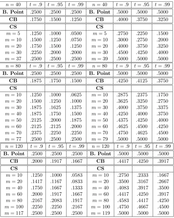
nontrivial breakdown point, to stay away from extreme quantiles, and to avoid small block sizes. Table 1 emphasizes this point by computing the subsampling quantile breakdown points when n= 40,80,120, and for b = 0.25,0.5. The bootstrap quantile breakdown points based on Singh (1998) formula are often close to the ones given by medium subsample sizes.
Insert Table 1 about here
Theorem 2 implies that we can always obtain a target upper quantile breakdown point ˆ
b ∈ (1/n, b] by selecting a suitable block size ˆm = ˆm(n, t, b,ˆb). The formula for the smallest block size ensuring a given upper breakdown point of subsampling quantiles is given below.
Corollary 3 For given t ∈(0,1), let ˆb ∈(1/n, b] be such that nˆb∈N. The smallest block size ˆ
m such that bt,n,mˆ ≥ˆb is given by
ˆ
m= infnm:P hX(n, m,ˆb−1/n)< mbi≥to.
Corollary 3 implies that, for ˆb = b, it is possible to obtain a breakdown point bt,n,m as large
as the one of the statistic Tn. As highlighted by Table 1, in order to achieve this goal, it is
not in general necessary to select a trivial block size m = n. For instance, when b = .25, for sample sizes n = 40,80,120, the maximal breakdown point is achieved with m = 37,77,117, respectively. When b = .5, and n = 40,80,120, it is instead achieved with m = 39,79,119, respectively.
According to Theorem 2, the block size m has to be sufficiently high, in order to avoid undesired subsampling breakdown properties. However, to get consistency in a general setting, a condition like m/n → 0 should hold as n, m → ∞ (see, for instance, Politis, Romano and Wolf, 1999). This means that the application of Corollary 3 is essentially relevant only for particular settings for which the consistency of the subsampling holds with m=O(n); see Wu (1990), and Remark 2.2.2 in Politis, Romano and Wolf (1999).
The asymptotic subsampling breakdown behavior is characterized as follows.
Corollary 4 Let subsampling block size m satisfy m/n → r ∈ [0,1), m, n → ∞. Then,
bt,n,m= b−zt
p
b(1−b)(1−r)/√m+O(1/m), for n large enough, where zt is the t−quantile
of the standard normal distribution.
From Corollary 4, the subsampling breakdown pointbt,n,mconverges to the breakdown point
of statistic T as n, m → ∞. Therefore, similar to the asymptotic bootstrap breakdown point formula in Singh (1998), Corollary 4 rules out the breakdown problem of subsampling quantiles for large samples and large subsampling block sizes.
2.2
Breakdown Point and Data Driven Choice of the Block Size
A main issue in the application of subsampling procedures is the choice of block sizem, because the subsampling accuracy heavily depends on this parameter. In this section, we study the robustness of data driven block size selection procedures based on either a minimization of the confidence interval volatility index (MCIV) or the calibration method (CM); see Romano and Wolf (2001).Given a sample of size n, we denote by M={mmin. . . , mmax} the set of admissible block sizes. Both MCIV (denoted by v) and CM (denoted by c) select the data-driven block size
mu ∈ M, with u=v, c, as solution of a problem of the form
mu = arg infm∈M{Fu,1(X1, . . . , Xn;m) :Fu,2(X1, . . . , Xn;m)∈Iu} , (3)
where by definition arg inf(∅) := ∞, Fu,1, Fu,2 are two scalar functions of the original sample (X1, . . . , Xn) and block sizem, and Iu is a subset of R; see equations (6) and (8) below for the
explicit definitions of Fu,1, Fu,2 in the setting u=v, c.
We characterize the robustness properties of MCIV and CM by their respectively breakdown points. More precisely, we are interested in computing the minimal proportion of contamination in the original sample such that the data driven choice of the block size fails and diverges to infinity. Consequently, we consider the following definition for the breakdown point:
Definition 5 The breakdown point of mu :=mu(X1, . . . , Xn) is defined as
but := inf{p∈[1/n, p] :np∈N and mu(Z1, . . . , Zn)→+∞}, (4)
where the sample (Z1, . . . , Zn) is obtained by replacing np data points Xi1, . . . , Xinp of the orig-inal sample (X1, . . . , Xn) by values Yi1, . . . , Yinp, with Yij → ±∞, j = 1, . . . , np.
In the next sections, we briefly describe the MCIV and CM approaches, and compute their breakdown points.
2.2.1 Minimum Confidence Interval Volatility Method
A consistent method for a data driven choice of mdetermines the block size by minimizing the confidence interval volatility index across the admissible values of m. For brevity, we present the method for one–sided intervals. Modifications for the case with two–sided intervals are obvious.
Definition 6 Let mmin < mmax, and k ∈Nbe fixed. Form∈ {mmin−k, . . . , mmax+k} denote by Q∗t(m) the (lower) t−subsampling quantile for block size m. Further, define Q∗tk(m) as the average quantile Q∗tk(m) := 2k1+1Pj=k
j=−kQ
∗
t(m+j). The confidence interval volatility (CIV)
index is defined for m∈ {mmin, mmin+ 1, ..., mmax−1, mmax} by
CIV(m) := 1 2k+ 1 j=k X j=−k Q∗t(m+j)−Q∗tk(m) 2 . (5)
LetM:={mmin, mmin+ 1, . . . , mmax}. The data driven block size that minimizes the confidence interval volatility index is
mv = arg infm∈M{CIV(m) :CIV(m)∈R+} , (6)
where, by definition, arg inf(∅) := ∞.
The block size mv minimizes the empirical variance of the upper bound in a subsampling
confidence interval with nominal confidence level t. Typical recommended choices for k, mmin andmmaxarek= 2,3,mmin =c1nζandmmax =c2nζ, respectively, wherec1 ∈[0.5,1],c2 ∈[2,3] and ζ = 0.5; see Romano and Wolf (2001). Moreoveor, according to Theorem 2, in order to ensure a minimal breakdown point for the quantile of the subsampling distribution, we can select the value of mmin as
where ˆm is the minimal subsampling block size in Corollary 3, which ensures a breakdown point larger than ˆb. Using Theorem 2, the formula for the breakdown point of mv follows from
Definition 5.
Corollary 7 For given t ∈ (0,1), let bt(m) be the subsampling upper t−quantile breakdown
point in Theorem 2, as a function of the block size m∈ M. Then we have:
bvt = sup
m∈M
inf
j∈{−k,..,k}bt(m+j).
Since mv is a crucial parameter for the accuracy of the resulting subsampling inference, it
is convenient to quantify bv
t for realistic applications. To this end, we can use Corollary 7. For
instance, for a sample size n= 100 and fort = 0.99, we obtain mmin = 8 andmmax= 25, using the average recommended choice in Romano and Wolf (2001), i.e., c1 = 0.75 and c2 = 2.5. For a statistic with breakdown point b = 0.1 and for k = 3, this parameter setting implies
bv
t = 0.03. In other words, three outliers out of a hundred data points are sufficient to break
down the data driven choice of m based on the MCIV index.
2.2.2 Calibration Method
Another consistent method for a data driven choice of the block size m can be based on a calibration procedure in the spirit of Loh (1987). As above, we present this method for the case of a one–sided confidence interval only. The modifications for two-sided intervals are obvious.
Definition 8 Fix t∈(0,1)and let(X1∗, . . . , Xn∗)be a bootstrap sample from(X1, . . . , Xn). For
each bootstrap sample, denote by Q∗∗t (m) the t−sub-sampling quantile according to block size
m. The data driven block size according to the calibration method is defined by
mc:= arg inf m∈M{|t−P ∗ [Tn≤Q∗∗t (m)]|:P ∗ [Q∗∗t (m)∈R]>1−t}, (8) where, by definition,arg inf(∅) :=∞, andP∗ denotes the probability with respect to the bootstrap distribution.
By definition, mc is the block size for which the bootstrap probability of the event {Tn ≤
Q∗∗t (m)} is as near as possible to the nominal level t of the confidence interval, but which, at the same time, ensures that the subsampling quantile breakdown probability of the calibration method is less than t. The last condition is necessary to ensure that the calibrated block size
mcdoes not imply a degenerate subsampling quantileQ∗∗t (mc) with a too large probability. By
definition, the breakdown point ofmcis the smallest fraction of outliers such that equation (8)
is degenerate, similar to the MCIV index method. The formula for the breakdown point of mc
is given next.
Corollary 9 Let t∈(0,1). The breakdown point of mc is given by bct = max m∈M{b
∗∗
t (m)}, with
b∗∗t (m) = inf{p∈[1/n, b] :np∈N and P [BIN(n, p)< nbt(m)]<1−t},
where bt(m) is for given m ∈ M the quantile subsampling breakdown point in Theorem 2 and
BIN(n, p) is a binomial random variable with parameters n and p.
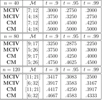
Table 2 compares the breakdown point ofmv and mc for some concrete parameter choices,
given a statistic with breakdown point b= 0.5.
Insert Table 2 about here
These theoretical results corroborated by unreported Monte Carlo results in linear regres-sion models indicate a higher robustness of the calibration method relative to the MCIV index method. Therefore, from a robustness perspective, the former should be preferred when consis-tent bootstrap methods are available. However, as discussed in Romano and Wolf (2001), the application of the calibration method in some settings can be computationally too expensive. In these cases, it is necessary to select an appropriate subset ofMfor the admissible block size (see Romano and Wolf (2001), Remark 5.4).
2.3
Robust Subsampling
To overcome the problem of the low breakdown point of subsampling quantiles, it is necessary first to apply subsampling methods to robust statistics, in order to avoid a trivial breakdown
point from the beginning, and, second, to robustify the subsampling procedure itself. We first show how this goal can be achieved for the class of robust M-estimators, by applying the fast subsampling approach in Hong and Scaillet (2006). Such a fast approach is put forward, among others, in Davidson and McKinnon (1999) and Andrews (2002) for the bootstrap. It can be used to extend in a convenient way the robust bootstrap procedure for fixed point estimators of Salibian-Barrera, Van Aelst and Willems (2006, 2007) to the robust subsampling setting with M-estimators. In a second step, we study in more detail the linear regression setting, where explicit breakdown point characterizations are possible. We develop robust subsampling procedures for robust MM-estimators and derive a formula for the implied subsampling quantile breakdown point. These results are a natural complement to the theoretical findings obtained in Salibian-Barrera and Zamar (2002) for the robust bootstrap.
We consider the class of robust M-estimators ˆθn for parameter θ ∈ Rd, defined by the
solution of ψn(ˆθn) = n X i=1 f(Xi,θˆn) = 0, (9)
for some functionψn:Rd→Rddepending on the parameterθand on the sample (X1, . . . , Xn),
where f is a known Rd-valued function. In particular, we focus on robust M-estimators with
bounded influence function, i.e., bounded estimating function f, see, e.g., Hampel, Ronchetti, Rousseeuw and Stahel (1986).
The boundedness of the estimating function is a key feature for developing our robust subsampling approach. As shown previously, a high breakdown point of ˆθn does not have to
imply a high breakdown point for the corresponding subsampling quantiles. For instance, in Table 1, we obtain very low breakdown points of subsampling quantiles, especially for small subsample sizes, even using robust estimators. A second issue is the fact that the application of robust estimators in resampling schemes can rapidly become prohibitive from a computational point of view.
To obtain a robust and computationally feasible subsampling method, we consider the following Taylor expansion of (9) around the true parameter value θ?: ψn(ˆθn) = ψn(θ?) +
∇ψn(θ?)(ˆθn−θ?) +oP(1), where ∇ψn ∈Rd×d is the matrix of partial derivatives with respect
to parameter θ. This implies: ˆθn−θ? = (−∇ψn(θ?))−1ψn(θ?) +oP(1). Thus, we can consider:
(−∇ψn(ˆθn))−1ψn,m∗ (ˆθn) as an approximation of ˆθn,m∗ −θˆn, where ψn,m∗ is computed from the
subsampling block (X1∗, . . . , Xm∗).
Given the normalization constant τn, the robust subsampling distribution approximating
the sampling distribution of τn(ˆθn−θ?) is defined by
LRn,m(x) = 1 Nn,m Nn,m X s=1 I n τm(−∇ψn(ˆθn))−1ψn,m,s∗ (ˆθn)≤x o , (10)
where sindexes the set of possible subsamples, Nn,m = mn
, and I{·}is the indicator function. The following standard high-level assumptions ensures consistency of the robust subsampling for the class of robust M-estimators; see also Politis, Romano, and Wolf (1999).
(A1) ˆθn =θ?+OP(1/τn).
(A2) (−∇ψn(ˆθn))−1 = (−∇ψn(θ?))−1+oP(1).
(A3) τn(ˆθn−θ?) =τn(−∇ψn(θ?))−1ψn(θ?) +oP(1).
(A4) There exists a limit lawJ(H) such that the distribution of τn(ˆθn−θ?) converges weakly
to J(H).
Given Assumptions (A1)-(A4), consistency of the robust subsampling scheme follows as stated in the next theorem.
Theorem 10 Let Assumptions (A1)-(A4) be satisfied. Assume further that τm/τn → 0 and
m/n→0 as m, n→ ∞. Then we get:
(1) If x is a continuity point of J(., H), then LRn,m(x)→J(x, H) as n→ ∞.
(2) If J(., H) is continuous, then supx|LR
(3) Given α∈(0,1) definecn,m(1−α) = inf{x:Ln,mR (x)≥1−α} and c(1−α, H) = inf{x:
J(x, H)≥1−α}. If J(., H) is continuous at c(1−α, H), then:
Phτn(ˆθn−θ?)≤cn,m(1−α)
i
→1−α, as n→ ∞ .
Statements 1–3 in Theorem 10 are standard statements on the weak convergence of the robust subsampling approximation to the true asymptotic distributionJ(H) of√n(θbn−θ?). Statement
3 implies that the (1−α)−quantile ofLRn,m converges to the corresponding (1−α)−quantile of
J(H). Therefore, the quantities cn,m(1−α),α ∈(0,1), can be used to construct finite sample
tests and confidence intervals for θ? with correct asymptotic size and coverage.
The robustness improvement provided by our robust approach is observable through the definition of the robust subsampling distribution (10). Indeed, in this definition we note that the subsampling quantile breakdown point is maximal if (i) (−∇ψn(ˆθn))−1 does not breakdown
as long as ˆθn does not breakdown, and (ii) given a subsampling block sizem, function ψn,m∗ (ˆθn)
is bounded with a bound that depends only on the original data set. The last condition is typically satisfied by the estimating functions of robust M-estimators. The first one is often verifiable in concrete model settings. In Section 2.4, we characterize explicitly the breakdown point of robust subsampling quantiles in the linear regression setting based on MM-estimates. The fast subsampling approach can be applied also with estimators ˜θndefined by the solution
of a set of smooth fixed-point equationsgn(˜θn) = ˜θn, for some functiongn:Rd→Rddepending
on the parameter θ and the sample (X1, . . . , Xn). This follows from writing the fixed-point
equations in the form gn(˜θn)−θ˜n = 0. This corresponds to equation (9) with ψn = (gn −
Id), where Id is the identity function Id(x) = x. Consequently, in these cases the robust subsampling is equivalent to the extension of the robust bootstrap approach in Salibian-Barrera, Val Aelst and Willems (2007) to the subsampling setting.
2.4
Robust Subsampling in the Linear Regression Model
We consider the iid linear regression model:Yi =Xi0β+σUi, i= 1, .., n, (11)
where Yi is a scalar random variable, Xi an Rd−valued random variable, β ∈ Rd, σ ∈ R+,
E[Ui] = 0, V ar(Ui) = 1, and E[UiXi] = 0. The joint probability distribution of (Yi, Xi0)
0 is
denoted by H. Several robust estimators of β and σ are available in the literature; see, e.g., Hampel et al. (1986) for a review. We focus on a high-breakdown MM-estimator of β (Yohai, 1987).
Let{(yi, x0i)
0 :i= 1, .., n}be a sample of observations of model (11). The MM-estimate
b
βn
of β is defined by the implicit equation:
1 n n X i=1 ∇ρ1 yi−x0iβbn b σn ! xi = 0. (12)
In equation (12), ∇ρ1 is the derivative of a continuously differentiable, bounded and sym-metric function ρ1, satisfying the assumption (A1)-(A4) below. The estimate bσn is a scale
S−estimate that minimizes with respect to β the M−estimate bσn(β), defined implicitly by
1 n n X i=1 ρ0 yi−x0iβ b σn(β)
= B, where function ρ0 satisfies the same assumptions as ρ1 and B is a
positive constant. We denote by ˜βn the S−regression estimate, i.e., σbn =bσn( ˜βn). The choice
of B determines the breakdown point of the estimators, which is maximal for B = 0.5 (see, e.g., Huber, 1981).
Note that the estimates ˆβn, ˆσn, and ˜βn satisfy the equations,
1 n n X i=1 ∇ρ1 yi−x0iβˆn b σn ! xi = 0, 1 n n X i=1 ρ0 yi−x0iβ˜n b σn ! =B, 1 n n X i=1 ∇ρ0 yi−x0iβ˜n b σn ! xi = 0. (13) Let ˆθn = ( ˆβn,ˆσn,β˜n). Simple calculations allow us to write the equations in (13) as a unique
compu-tation of function gn. Therefore, as discussed in the previous section, we can apply our robust
subsampling approach to this setting. We first introduce the following notation.
Notation 11 (i) For i = 1, .., n, define the residuals: bri =yi−x0iβbn and r˜i = yi −x0iβ˜n, and
compute the weights: ωbi = ∇ρ1(bri/σbn)/rbi, ˜vi = b
σn
nBρ0(˜ri/σbn)/r˜i. (ii) Given m < n, define for
every subsampling block{(y∗i, x∗i0) :i= 1, .., m}the residualsbr∗i =y∗i−x∗i0βbnandr˜∗i =yi∗−x∗i0β˜n,
and compute the weights:
b ωi∗ =∇ρ1(rb ∗ i/bσn)/br ∗ i, v˜ ∗ i = b σn nBρ0(˜r ∗ i/σbn)/r˜ ∗ i. (14)
With these weights, define:
b βn,m∗ = m X i=1 b ω∗ix∗ix∗i0 !−1 m X i=1 b ω∗ix∗iyi∗, bσ∗n,m = m X i=1 ˜ vi∗(yi∗−x∗i0β˜n). (15)
Note that the weights bωi and ˜vi are computed without recalculating the estimators βbn, ˜βn and
b
σn, and are kept fixed for each subsampling block. Because of this construction, the quantities
b
βn,m∗ andσbn,m∗ in (15), which are only an approximation of the “true” point estimatesβbm∗ andbσ∗m
implied by the subsampling block{(y∗i, x∗0i ) :i= 1, .., m}, may not reflect the actual variability of ˆβnand ˆσn. We overcome this problem by applying the linear correction factors defined in (17)
and (18) below. In this way, the large breakdown point of these estimators will be inherited by the implied subsampling quantiles. Moreover, since it is not necessary to compute the implied robust point estimate in each subsampling block, the robust subsampling in Definition 12 yields a computationally feasible resampling scheme. This allows us to compute robust confidence intervals for the regression parameter β in presence of the nuisance scale parameter σ.
Definition 12 Letβ? be the true parameter value in the regression model (11) andJn(H)be the
sampling distribution of √n(βbn−β?), i.e., for any x∈Rn: Jn(x, H) =P
h√
n(βbn−β?)≤x i
. The robust subsampling approximation of Jn(x, H) is given by
LRn,m(x) = 1 Nn,m Nn,m X s=1 I n Mn √ m(βbn,m,s∗ −βbn) +dn √ m(bσ∗n,m,s−bσn)≤x o , (16)
where the linear corrections Mn and dn are defined as follows: Mn = bσn n X i=1 ∇2ρ 1(rbi/bσn)xix 0 i !−1 n X i=1 b ωixix0i, (17) dn = nB b σ2 n n X i=1 ∇ρ0(˜ri/σbn)˜ri/bσn n X i=1 ∇2ρ 1(bri/bσn)xix 0 i !−1 n X i=1 ∇2ρ 1(bri/bσn)brixi. (18)
The following are detailed assumptions on the robust linear regression setting based on the above MM-estimator, which ensure consistency of the robust subsampling approximation in Definition 12.
(A5) The sampling distributionJn(H) converges weakly to a limit distributionJ(H) asn → ∞.
(A6) The following limits in probability hold as n → ∞: βbn→β?, ˜βn→β˜?, b
σn → σ?, where
parameters β?,β˜? and σ? are the unique solution of the set of moment conditions:
E[∇ρ1((Y1−X10β)/σ)] = 0, E h ρ0((Y1−X10β˜)/σ) i =B, Eh∇ρ0((Y1−X10β˜)/σ) i = 0.
(A7) Forj = 0,1, the functionρj is three times continuously differentiable and such that: (R1)
ρj(−u) = ρj(u) for all u ∈ R; (R2) ρj(0) = 0; (R3) supu|ρj(u)| = 1; (R4) If ρj(u) < 1
and 0< v < u then ρj(v)< ρj(u).
(A8) Let r=Y1−X10β?. The following matrices exist and are finite:
E ∇ ρ1(r) r X1X 0 1 −1 , E[∇ρ1(r)X1X10], E ∇2ρ 1(r)X1X10 −1 , (19) E[∇ρ1(r)rX1X10], E ∇ ρ0(r) r X1X 0 1 −1 , E[∇ρ0(r)r], (20) E ∇2ρ 0(r)X1X10 , E ∇2ρ 0(r)rX1 , E ∇2ρ 1(r)rX1 . (21)
In addition, the third matrix in (20) is not zero.
(A9) The following functions are continuous:
u7−→ ∇ρ0(u) u , u7−→ ∇ρ0(u)− ∇2ρ0(u)u u2 , u7−→ ∇ρ1(u)− ∇2ρ1(u)u u2 .
A well-known example where assumptions (A1)-(A9) are typically satisfied arises for func-tions ρ in the Tukey’s family:
ρ(u) =
3(u/d)2−3(u/d)4+ (u/d)6, if |u| ≤d,
1 if |u|> d,
where d >0 is a fixed constant; see also Salibian-Barrera and Zamar (2002). We use a MM-estimator based on such functions in the Monte Carlo experiments reported below for the linear regression. Consistency of the robust subsampling in Definition 12 is stated in the next theorem.
Theorem 13 Let Assumption (A5)-(A9) be satisfied. Then we get:
1. Ifxis a continuity point ofJ(·, H), then the following limit in probability holds asn, m→ ∞ and m/n→0: LRn,m(x)→J(x, H).
2. If J(·, H) is continuous, then the following limit in probability holds as n, m → ∞ and
m/n→0: sup
x
|LRn,m(x)−J(x, H)| →0.
3. For α ∈ (0,1), define cn,m(1−α) = inf{x : LRn,m(x) ≥ 1−α}, c(1−α, H) = inf{x :
J(x, H)≥ 1−α}. If J(·, H) is continuous at c(1−α, H), then the following limit holds as n, m→ ∞ and m/n→0: P h√n(βbn−β?)≤cn,m(1−α)
i
→1−α.
In contrast to the general M-estimator case, we can exploit the additional structure of the linear regression setting to explicitly characterize the breakdown point of robust subsampling quantiles. The breakdown point formula for the robust subsampling in Definition 12 is given in the next theorem.
Theorem 14 Let √ωb1x1, .., √
b
ωnxn be in general position, i.e., any d row vectors of then×d
design matrix X = [√bωix0i]i=1,..,n are linearly independent, and fix t ∈(0,1).
1. The breakdown point bRt,n,m of the t−quantile of the robust subsampling in Definition 12 is given by
where b is the breakdown point of the robust M M−regression estimator βbn.
2. LetbbR ∈(1/n, b] be such thatnbbR ∈N. The smallest block size b mR such that bR t,n,mˆR ≥bbR is given by b mR= inf{m:P hX(n, m,bbR−1/n)≤m−d i ≥t}.
The assumption on the general position of √ωb1x1, .., √
b
ωnxn is also used in Salibian-Barrera
and Zamar (2002), and is needed here to ensure that the approximation βbn,m∗ of the
subsam-pling estimate βbm∗ is well-defined in every subsampling block. By comparing (22) with the
breakdown formula (2) of the standard subsampling in Theorem 2, we note that for reason-able parameter choices mb << m− d = m(1− d/m). Therefore, P [X(n, m, p)< mb] << P [X(n, m, p)≤m−d] and bR
t,n,m>> bt,n,m. The numerical difference between the two
break-down points can be large. Table 3 computes the robust subsampling breakbreak-down point for a setting withd= 3 and for sample sizesn= 40,80,120, in dependence of the breakdown pointb
of theM M−regression estimatorβbn. We find that statement 2 of Theorem 14 can be more
rele-vant for applications than the one of Corollary 3. This is so because a large breakdown point of the robust subsampling can arise also for small subsampling block sizes, which asymptotically can more easily ensure the subsampling consistency conditions.
Insert Table 3 about here
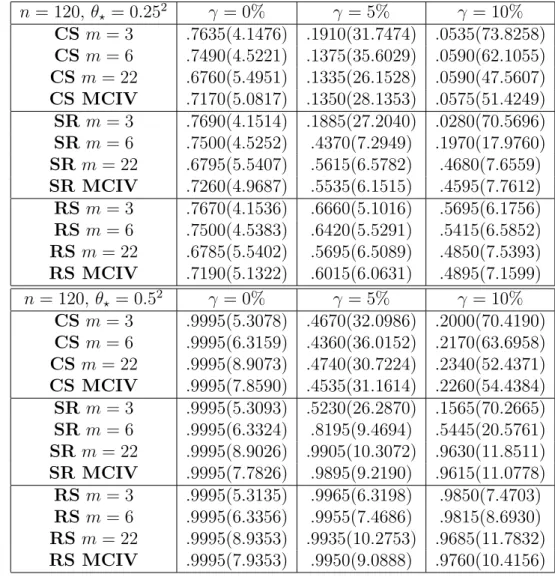
For b = 0.225 and n = 40, the robust subsampling breakdown point is bRt,n,m = 0.225 for all m ≥ 6. For t = 0.9, the maximal breakdown point is obtained already for m = 8. For
t = 0.95 and t = 0.99, it is obtained for m = 10 and m = 12, respectively. In general, the maximal breakdown point is obtained for all samples sizes and confidence levels in Table 3, independently ofb, form= 14. Whenb <0.5, the value ofmensuring the maximal breakdown point is even lower. These are large differences with respect to the subsampling breakdown points in Table 1.
These results have implications also for the breakdown point of mv in Corollary 7. For
(2001) yields mmin = 8 and mmax= 25 (using c1 = 0.75 and c2 = 2.5). For b = 0.1 and k = 3, the breakdown point of mv when using the robust subsampling is maximal for all confidence
levels, but the one when using the standard subsampling is bvt = 0.03 for t = 0.99. On the other side, the breakdown point of mc is much higher, as was shown by our previous numerical
computations.
Our results on the robust subsampling extend directly to linear regression models with fixed designs. Assume that the covariates Xi ∈ Rd are fixed and part of an infinite sequence
(X1, . . . , Xn, Xn+1, . . .). ForZi = (Yi, Xi0)
0, letH be the joint probability law governing the
in-finite sequence (Z1, . . . , Zn, Zn+1, . . .). Salibian-Barrera (2006a) proves consistency and asymp-totic normality of MM-estimators in this setting. Moreover, Salibian-Barrera (2006b) shows the validity of the first order Taylor expansion for the corresponding fixed-point estimating equation. Under the weak assumptions of Theorem 4.3.1 in Politis, Romano and Wolf (1999), the consistency of the robust subsampling in Definition 16 then follows even for settings with fixed designs.
3
Monte Carlo Study and Sensitivity Analysis
We study through Monte Carlo simulations the statistical properties (size and power) of the subsampling and the robust subsampling in estimating the confidence interval of (i) the squared mean for an iid sample and (ii) a parameter of interest in the iid linear regression model (11) when this parameter is possibly near a boundary. In both settings, the bootstrap is inconsistent, but subsampling procedures are applicable.
3.1
Squared mean
The first example concerns the sampling distribution of the squared mean for an iid normal sample with known variance. This is an informative, albeit simple, design to measure the accuracy of subsampling techniques in presence of model contaminations. As discussed, e.g., in Datta (1995), the bootstrap fails in this setting, and only a modified bootstrap procedure
is applicable. Instead, the subsampling is consistent without modifications of the standard procedure.
3.1.1 Model and Estimation
Let (X1, . . . , Xn) be an iid sample with Xi ∼ N(µ,1), and take the parameter of interest as
θ =µ2. Let the nonrobust estimator ˆθN R
n be the squared sample average ˆθnN R= n1
Pn
i=1Xi
2
, so that the asymptotic distribution of nθˆN R
n is a non-central chi-squared distribution with one
degree of freedom and noncentrality parameter µ2. Let (X∗
1, . . . , X
∗
m) be a random subsample
such that the subsampling statistic is ˆθN R,∗
n,m = 1 m Pm i=1X ∗ i 2
. We denote by θ? the true
parameter value. Then, the subsampling approximation of the distribution of n(ˆθN R
n −θ?) is LCSn,m(x) = 1 Nn,m Nn,m X s=1 I n m(ˆθn,m,sN R,∗ −θˆnN R)≤xo. (23)
We refer to using (23) as “classical subsampling (CS)” . Let us now consider a robust estimator ˆθR
n based on the square of the robust location
estimate ¯XnR given as solution of the equation ψn( ¯XnR) = 0, where functionψn is defined by
ψn(θ) = 1 n n X i=1 hc(Xi−µ), (24)
and hc(x) = x·min(1, c/|x|) is the Huber function. We denote by ˆθR,n,m∗ the robust estimator
based on the random subsample. Then, the subsampling approximation of the distribution of
n(ˆθR n −θ?) is LSRn,m(x) = 1 Nn,m Nn,m X s=1 I n m(ˆθn,m,sR,∗ −θˆRn)≤xo. (25) We refer to using (25) as “subsampling robust (SR)”. As discussed in the introduction, sub-sampling a robust estimator does not deliver a robust resub-sampling procedure.
To robustify subsampling, we use the decomposition m(ˆθR,∗
n,m −θˆRn) = m(( ¯XR, ∗ n −X¯nR)2 + 2 ¯XR n( ¯XR, ∗ n −X¯nR)), where ¯XR, ∗
n is the subsampling robust estimator of the true mean µ?. Then,
using our robust approach, the idea is to consider An,m,s = (−∇ψn( ¯XnR))
−1ψ∗
approximation of ¯XnR,∗ −X¯nR. The robust subsampling approximation of the distribution of n(ˆθR n −θ?) is obtained as LRSn,m(x) = 1 Nn,m Nn,m X s=1 Im(A2n,m,s+ 2 ¯X R nAn,m,s)≤x . (26)
We refer to using (26) as “robust subsampling (RS)”.
3.1.2 Numerical Results
We consider a sample size n = 120. Results are almost identical for n = 40,80. Since the calibration method is not applicable here (bootstrap inconsistency), we use a data driven block size obtained by minimizing the CIV index for k = 2. Forn = 120, the minimal recommended choice in Romano and Wolf (2001) implies a lower bound mmin = 6 and an upper bound
mmax= 22, for c1 = 0.5 and c2 = 2, respectively. Beside these selections, we consider also the block size m= 3 as extreme case.
We study the finite sample coverage implied by subsampling (CS, SR), and robust subsam-pling (RS). To this end, we test the null hypothesis H0 :θ? = 0 against H1 :θ? >0, under the
following data generating process for Xi:
Xi ∼(1−γ)N(µ?,1) +
γ
2(N(5,100) +N(−5,100)),
for γ = 0 (no contamination), γ = 0.05 (5% of contaminated data) and γ = 0.10 (10% of contaminated data). We use the true value µ? = 0 for the size, and µ? =.25, .5 for the power.
For each of the 2000 Monte Carlo replications, resampling distributions are computed based on 200 draws. For the subsampling approximations we generate the 200 draws, instead of the
Nn,m possibilities, by permuting the original sample and taking the first m observations of the
random samples. Table 4 and Table 5 summarize the empirical frequencies of rejection of the null hypothesis H0 for a significance level α=.05.
Let us first analyze the size issues summarized in Table 4. We find that the empirical frequencies for the robust subsampling are quite accurate and closer to the nominal frequencies
than those of the other resampling methods. Under a model contamination, the underrejection of the null hypothesis using classical subsampling can be severe: We get an empirical rejection frequency less than.02 instead of the true.05 value whenγ = 0.10. According to the theoretical results, Table 4 confirms that resampling a robust statistic does not yield a robust resampling method. Indeed, for m= 3, and γ = 0.05,0.10, the results implied by SR are even worse than those implied by CS. The robustness problem of SR can be in part mitigated by the selection of a larger block size (m = 22), nevertheless our robust approach still outperforms SR. At the same time, the quantile implied by the classical subsampling virtually explodes in presence of contamination, leading to a virtually noninformative inference. For instance, when γ = 0.10, and m = 3, the median .95-quantile implied by the classical subsampling approximation is 71.55, while the one implied by the robust subsampling approximation is 5.75.
Finally, in Table 5 we can analyze the power of the procedures under investigation. When
θ? > 0, the proportion of rejection of H0 increases as expected. Without contamination all the procedures under investigation imply similar accurate results. When γ >0, the proportion of rejections implied by the classic approach dramatically decreases. For instance, when θ? =
0.252, γ = 0.10, and m = 6, the power of CS and SR are less than 6% and 20%, respectively. For our robust approach, in the same case, the power is instead larger than 54%.
Unreported Monte Carlo results for the bootstrap approach confirm the inconsistency of this method in the squared mean setting. In particular, we consider a nonrobust approximation similar to (23), and the robust approximations similar to (25) and (26), but based on the bootstrap instead of the subsampling approach. When θ? = 0, tests based on these three
bootstrap distributions never reject H0 both in presence or absence of contaminations.
Insert Table 4 and Table 5 about here
3.2
Linear Regression
In this section we consider the iid linear regression model (11) when a parameter of interest is possibly near a boundary (see, e.g., Kim, Stone and White (2005) for an application in finance). As discussed in detail by Andrews (2000), the bootstrap is inconsistent in this context and the
subsampling is a potentially natural alternative to it. Moreover, Andrews and Guggenberger (2009a, 2010a,b) (see also Mikusheva (2007) for a similar problem in autoregressive models with unit roots) show that pure subsampling methods have a lack of uniform asymptotic approxi-mation within a class of models including our Monte Carlo setting. They also develop hybrid and size-correction procedures to fix the arising asymptotic size distortion. Analogous remarks hold in the linear regression model when making inference on a parameter of a given regressor and the parameter of another regressor, a nuisance parameter, may be near a boundary. We follow their hybrid approach in our Monte Carlo study of the classical and robust subsampling.
3.2.1 Model and Estimation
We consider the scalar regression parameter β, which is known to satisfy the constraint β ≥0 in the iid linear regression model:
Yi = Xi0θ+Wiβ+σUi,
= Zi0η+σUi, i= 1, . . . , n, (27)
where Yi, Wi are scalars, Xi is an Rd−1-valued random variable, θ ∈ Rd−1, and σ ∈ R+.
Moreover, Zi(1) =Xi(1) = 1, η(1) =θ(1), Zi(2) =Wi, η(2) =β and for 3 ≤j ≤d, Zi(j) =Xi(j−1),
η(j)=θ(j−1), whereh(j) denotes thej-th coordinate of vectorh. In order to construct confidence intervals for parameter β using the classic subsampling, we consider the constrained estimator
ˆ
βN R
n = max(0,ηˆnols(2)), where ˆη
ols
n is the (unrestricted) OLS estimator of η. For the robust
subsampling, we consider the constrained estimator ˆβnR = max(0,ηˆnrob(2)), where ˆηrobn is a MM-estimator of η. The S-estimate ˆσn= ˆσn(˜ηrobn ) is computed from a constrained robust estimator
˜
ηnrob of η under the constraintη(2) ≥0.
We construct consistent subsampling and robust subsampling methods as follows. For the subsampling, we compute in each block the constrained estimator ˆβn,mN R = max(0,ηˆn,mols (2)). The subsampling distribution function estimating the distribution function of√n( ˆβN R
given by LN Rn,m(x) = 1 Nn,m Nn,m X s=1 I n√ m( ˆβn,m,sN R −βˆnN R)≤xo. (28)
For the robust subsampling, we follow (15) and (16) and additionally account for the parameter constraint. Thus, we consider the robust subsampling statistic
ˆ subβ∗n,m = max (Mn(ˆη∗n,m−ηˆ rob n ) +dn(ˆσn,m∗ −σˆn))(2)+ ˆβnR,0 .
The robust subsampling distribution function which approximates the distribution function of √ n( ˆβnR−β?) is then given by LRn,m(x) = 1 Nn,m Nn,m X s=1 I n√ m( ˆsubβ∗n,m,s−βˆnR)≤xo. (29)
By construction, the theoretical results in Section 2.4 for the upper quantile breakdown point of the robust subsampling distribution in Definition 12 hold also for (29).
3.2.2 Hybrid Procedures
Using (28) and (29), we construct hybrid, classical and robust, equal-tailed confidence intervals for parameter β as follows. Let cn,m(1−α) be the (1−α)-quantile implied by either (28) or
(29). The corresponding hybrid quantile is:
cHn,m(1−α) = max(cn,m(1−α), c∞(1−α)), (30)
where c∞(1−α) is the quantile of the asymptotic distribution of
√
n( ˆβni −β?), i=CL, R, for
the unconstrained, either classical or robust, estimator ˆβi
n ofβ. To compute c∞(1−α), we can
use standard asymptotic normality results for OLS estimators and the asymptotic normality results for MM-estimates in Yohai (1987). However, Salibian-Barrera and Zamar (2002) show that these asymptotic approximations behave poorly in presence of contamination. Therefore, we use the bootstrap and the robust bootstrap, for the subsampling and the robust subsampling,
respectively, to estimate the distribution of the unconstrained estimators in the computation of hybrid quantiles. Unreported numerical results confirm the superiority of this approach. In this way, the construction of hybrid quantiles for our robust subsampling approach can profit also from the robustness properties of the robust bootstrap developed in Salibian-Barrera and Zamar (2002).
3.2.3 Numerical Results
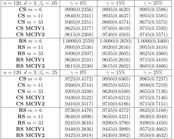
We consider the iid linear regression model (27) for d= 3,5 and n = 120. Results are almost identical for n = 40,80. The true parameter vector is η? = (0, β?,0)0 and η? = (0, β?,0,0,0)0,
respectively, with β? = .05, .25. We analyze the accuracy of subsampling procedures for fixed
and data driven block sizes. For our sample size n = 120, the maximal recommended choice in Romano and Wolf (2001) implies a lower bound mmin = 6 and an upper bound mmax= 33, for c1 = 0.5 and c2 = 3, respectively. Nevertheless, because of convergence problems of the algorithm, for d = 5 block sizes less than m = 8 are not applicable. Besides the selections recommended by Romano and Wolf (2001), we analyze also the accuracy of the block sizes implied by Theorem 14. In particular, we consider the block sizes m = 11 and m = 16, for
d = 3 and d = 5, respectively, which imply a breakdown point of 50% for the .975-quantile. Finally, since the calibration method is not applicable here, we use a data driven block size obtained by minimizing the CIV index with k = 2. More precisely, for d = 3 we apply MCIV to the intervals I(d=3,1) ={8, . . . ,27} and I(d=3,2) = {11, . . . ,27}, while for d = 5, we consider the intervals I(d=5,1) = {10, . . . ,27} and I(d=5,2) = {16, . . . ,27}. The intervals I(d=3,1) and
I(d=5,1) represent the average intervals proposed by Romano and Wolf (2001) for this setting. The intervals I(d=3,2) andI(d=5,3) represent instead the optimal intervals based on Theorem 14, which ensure a breakdown point of 50% for the .975-quantile.
We make use of functionsρ0 and ρ1 in Tukey family. The constant for the M M−regression estimator in our simulations is B = 0.5. For this choice, we obtain a breakdown point of bηn
satisfying b ≥0.47; see Yohai (1987, Theorem 2.1).
robust subsampling methods (denoted by CS and RS, respectively). We do not report results concerning SR since its implementation is computationally prohibitive. The simulation results obtained in the previous squared mean regression example, as the theoretical results provided by our study, are convincing enough in showing that the application of the classical subsampling to the robust MM-estimator is not sufficient to imply a robust subsampling inference for this setting.
We consider parameter choicesβ? =.05, .25 under a contaminated distribution for U:
U ∼(1−γ)N(0,1) + γ
2(N(C,(0.1)
2) +N(−C,(0.1)2)), (31)
where C = 5, γ = 0 (no contamination), γ = 0.15 (15% of contaminated data) and γ = 0.25 (25% of contaminated data), as in Salibian-Barrera and Zamar (2002). For each of the 2000 Monte Carlo replications, resampling distributions are computed based on 500 draws. For the subsampling approximations we generate the 500 draws, instead of the Nn,m possibilities, by
permuting the original sample and taking the first m observations of the random samples. Table 6 and Table 7 summarize the empirical coverage for parameter choices β? = .05, and
β? = .25, respectively, and the median confidence interval lengths for the nominal confidence
level 1−α=.95.
Insert Table 6 and Table 7 about here
In all Monte Carlo simulation settings, the empirical coverage for the robust subsampling with data driven choice of the block size are accurate and closer to the nominal coverage than those of the classical subsampling. The median length of the robust subsampling confidence intervals is moderately higher in the setting with no contamination (γ = 0%). For instance, for the case n = 120, d = 3, β? = .25, the median confidence interval of the robust subsampling
is approximately 9% higher than the median length of the subsampling. However, in presence of contamination, the robust subsampling produces clearly a more efficient inference with dra-matically smaller median confidence interval lengths. For instance, for the casen= 120,d= 3,
lower than the median length of the subsampling when γ = 15% (γ = 25%). These are large differences having obvious implications for the power of tests based on subsampling and robust subsampling methods. Therefore, for the sake of brevity, we do not report a detailed power comparison of tests based on the two methods.
Unreported results for the inconsistent bootstrap and robust bootstrap yield empirical cover-ages between 51.35% to 56.50%, for parameterβ? =.05. Similarly, the subsampling and robust
subsampling without hybrid correction yield empirical coverages between 48.20% and 53.15%, which are not too far away from the theoretical distorted coverage (1−α)/2 of equal-tailed confidence intervals; see Andrews and Guggenberger, 2010b. Results of the robust bootstrap and hybrid robust subsampling for the parameter choiceβ? = 0.5 are more similar, as expected,
but still in favour of the latter. Unreported results with different contamination sizes, model dimensions and sample sizes (e.g., C = 4 , d= 20) produce similar results.
We complete this analysis with some results also for the naive bootstrap approach based on unconstrained estimators. More precisely, we compute a nonrobust bootstrap distribution by applying the classical bootstrap approach to the unconstrained OLS estimator of β. Similarly, we compute a robust bootstrap distribution by applying our robust approach to the robust unconstrained MM-estimator of β. Finally, we construct nonrobust and robust confidence intervals for the parameter of interest by truncating at 0 the confidence intervals implied by the unconstrained nonrobust and robust bootstrap distributions, respectively. As discussed in Andrews and Guggenberger (2010b) in relation to using the unconstrained OLS estimator, when
β? is ”sufficiently” far from the boundary restriction, confidence intervals computed in this way
may imply an empirical coverage quite close to the nominal confidence level. In contrast, for β?
”close” to the boundary this approach tends to produce too conservative confidence intervals. In our setting, forβ? =.25, d= 3, the robust bootstrap shows a desirable stability, implying an
empirical coverage between 94.4% and 96.1% both in presence and absence of contamination. The results for the nonrobust bootstrap confirm the lack of robustness of this method. Indeed, for β? = .25, the coverage ranges between 94.10% and 97.95%, for γ = 0 and γ = 0.25,
respectively. As expected the accuracy of both procedures deteriorates for β? = .05. In this
even without contamination.
Finally, to analyze the robustness properties of classical and robust subsampling with larger sample sizes, we also consider the case n = 500. Table 8 summarizes the empirical coverage for parameter choices β? =.05, .25, and the median confidence interval lengths for the nominal
confidence level 1−α=.95.
Insert Table 8 about here
We consider the maximal recommended choice proposed by Romano and Wolf (2001),
mmin = 12 and mmax = 68, respectively. Moreover, we also apply MCIV to the interval
I ={23, . . . ,45}, which represents the minimal interval proposed by Romano and Wolf (2001). In this setting, the block sizes m = 11 and m = 16 imply a breakdown point of 50% for the
.975-quantile for d = 3 andd= 5, respectively.
The Monte Carlo results confirm the findings obtained for smaller sample sizes. In particu-lar, we observe that classical and robust subsampling perform very similarly without contam-ination. Also, in this setting, the presence of contamination dramatically increases the length of classical subsampling confidence intervals. For instance, for d= 3 and β? =.25, the median
confidence interval of the robust subsampling is approximately 55% lower than the median length of the classical subsampling when γ =.25.
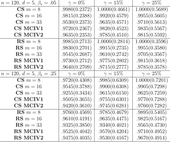
We have also studied the sensitivity of the subsampling and robust subsampling inference with respect to empirical contaminations of the data. For each Monte Carlo sample, let:
Ymax= arg max
Y1,...,Yn
{u(Yi)|u(Yi) = Yi−Zi0η,underH0 :β? = 0.25}. (32)
We modify Ymax over a grid within the interval [Ymax + 1, Ymax + 4]. Then, we analyze the sensitivity of the resulting empirical averages of p-values for testing the null hypothesis H0 :
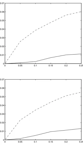
β? = 0.25. Figure 1 summarizes the results for n = 120.
Insert Figure 1 about here
As expected, we obtain quite large absolute variations in averagep-values for the subsam-pling and an almost flat sensitivity curve for the robust subsamsubsam-pling.
Finally, as a last exercise, we have computed the averagep−value for Monte Carlo samples generated under H0 : β? = 0.25, with increasing contamination sizes γ ∈[0,0.25] in (31) with
C = 15, and have analyzed the averagep−value variation with respect to the setting with no contamination (γ = 0). Figure 2 summarizes the results.
Insert Figure 2 about here
Also in this case, the subsampling clearly implies larger variations in average p-values as a function of the size of contamination in the data, indicating the fragility of the implied inference results.
4
Concluding Remarks
We derive a formula for the breakdown point of subsampling quantiles, which is shown to imply fragile subsampling procedures for moderate block sizes, even when subsampling is applied to robust statistics. This instability is inherited by data driven block size selection procedures. We propose consistent robust subsampling methods for the class of M-estimators and derive detailed breakdown point formulas for MM-estimators in the linear regression setting. Monte Carlo simulations in two settings where the bootstrap is known to fail show the usefulness of robust subsampling relative to the classical subsampling for producing accurate inferences in presence of model deviations.
Appendix: Proofs
Proof of Theorem 2. The quantile Q∗t,n,m breaks down if and only if the proportion of bounded realizations of the statisticTn,m∗ is less thant, i.e., when the proportion of subsamples with less than mboutliers is less thant. LetX(n, m, p) be the number of outliers in subsample (X1∗, . . . , Xm∗), when np is the number of outliers in the original sample (X1, . . . , Xn). The
random variableX(n, m, p) follows a hypergeometric distribution with parametersn,np, andm. Consequently, bt,n,m is the smallest proportion p such that np ∈ and P[X(n, m, p)< mb]< t,
which is the stated result.
Proof of Corollary 3. Existence of ˆm is ensured by Theorem 2. For a hypergeometri-cally distributed variable X(n, m, p) such that np ∈ N, the probability P[X(n, m, p)< mb] is decreasing in p. Consequently, bt,n,mˆ ≥ ˆb. By definition, for every integer m < mˆ,
P
h
X(n, m,ˆb−1/n)< mb
i
< t, and bt,n,m ≤ˆb−1/n. This concludes the proof.
Proof of Corollary 4. Let us take p = b − zt
p
b(1−b)(1−r)/√m + c/m, for p ∈ [0, b], and compute a Berry-Esseen type bound for the normal approximation of the hy-pergeometric distribution, where c is in a fixed compact set. For n and c large enough,
P [X(n, m, p)< mb] < t, where X(n, m, p) is a hypergeometric random variable with parame-ters n,np, and m. Forn large enough andcsmall enough,P [X(n, m, p)< mb]> t. Therefore,
bt,n,m=b−zt
p
b(1−b)(1−r)/√m+O(1/m), as stated.
Proof of Corollary 7. By definition, in order to get mv =∞ we must have CIV(m) = ∞
for all m ∈ M. Given m ∈ M, CIV(m) = ∞ if and only if the fraction of outliers p in the sample {X1, . . . , Xn} satisfies p ≥ min{bt(m−k), bt(m−k+ 1), .., bt(m+k−1), bt(m+k)}.
This concludes the proof.
Proof of Corollary 9. By definition, in order to getmc =∞we must haveP [Q∗∗t (m) = ∞]≥
at least as large as nbt(m). The number of outliers in the bootstrap sample is distributed as
B(n, p). This concludes the proof.
Proof of Theorem 10. Under Assumptions (A1)-(A4) the statements of the theorem follow from Theorem 1 in Hong and Scaillet (2006).
Proof of Theorem 13. We first rewrite the estimator ˆθn = (βbn0, b
σn,β˜n0)
0 as the fixed point
of the following system of equations:
b βn = An(βbn, b σn)−1Vn(βbn, b σn), b σn = σbnUn( ˜βn,bσn), ˜ βn = Bn( ˜βn,bσn) −1W n( ˜βn,σbn), (33) where An(β, σ) = 1 n n X i=1 ∇ρ1((yi−x0iβ)/σ) yi−x0iβ xix0i, Vn(β, σ) = 1 n n X i=1 ∇ρ1((yi−x0iβ)/σ) yi−x0iβ yixi, Un( ˜β, σ) = 1 n n X i=1 ρ0((yi−β˜0xi)/σ) B(yi−β˜0xi) (yi−β˜0xi), and Bn( ˜β, σ) = 1 n n X i=1 ∇ρ0((yi−x0iβ˜)/σ) yi−x0iβ˜ xix0i, Wn( ˜β, σ) = 1 n n X i=1 ∇ρ0((yi−x0iβ˜)/σ) yi−x0iβ˜ yixi.
Fn:R2d+1 →R2d+1. A first order expansion of (33) gives
√
n(ˆθn−θ?) = [I − ∇Fn(θ?)]
−1√
n(Fn(θ?)−θ?) +oP(1), (34)
where θ? = (β?0, σ?,β˜?0)0. The explicit computation of ∇Fn shows that ˜βn does not enter (34)
in the approximation of the first d+ 1 components of √n(ˆθn−θ?), i.e., the approximation of
√
n(βbn−β?) and
√
n(σbn−σ?). The d×d matrix Mn in (17) is the left upper diagonal block
of [I− ∇Fn(τn)]−1, and the vector dn in (18) is the d+ 1−th upper d−dimensional column of
this matrix. Summarizing, we obtain the approximation:
√ n(βbn−β?) = Mn,? √ n(An(β?, σ?)−1Vn(β?, σ?)−β?) +dn,? √ n(σ?Un( ˜β?, σ?)−σ?) +oP(1) =: ξn(θ?) +oP(1),
whereMn,? and dn,? are the same matrix and the same vector as in (17) and (18), respectively,
but evaluated at θ? instead of ˆθn. Therefore, we have to show that the limit distribution of
ξn(θ?) is the same as the limit distribution of
ξn,m∗ = Mn √ m(A∗n,m(βbn, b σn)−1Vn,m∗ (βbn, b σn)−βbn) +dn √ m(bσnUn,m∗ ( ˜βn,bσn)−bσn) = Mn √ m(βbn,m∗ −βbn) +dn √ m(bσ∗n,m−bσn).
To this end, it is sufficient to prove that the limit distribution ofζn,m∗ (ˆθn) :=
√
m(Fn,m∗ (ˆθn)−θˆn)
is the same as the limit distribution ofζn(θ?) :=
√
n(Fn(θ?)−θ?). In order to obtain this, we only
need to show that theU-statistic defined byUn,m(x) =
1 Nn,m Nn,m X s=1 I n√ m(Fn,m,s∗ (ˆθn)−θ?)≤x o
converges to the limit cumulative distribution of ζn(θ?), evaluated at any continuity point x.
This implication follows, however, with standard arguments; see, e.g., the proof of Theorem 2.2.1 in Politis, Romano and Wolf (1999).
Proof of Theorem 14. Under the assumptions of the theorem, we can use the same argu-ments as in the proof of Theorem 2 in Salibian-Barrera and Zamar (2002) to show that, given a subsampling block of sizem, the approximation βbn,m∗ is bounded, with a bound that depends
only on the original data set, if at least d observations in the block are not outliers. More-over, σ∗n,m remains bounded for every subsampling block. Therefore, the robust subsampling approximation in Definition 12 breaks down if and only if in the subsampling block the number
X(n, m, p) of outliers is larger than m−d. The proportion p of outliers in the original sample that is needed to drive the t−th subsampling quantile estimate above any bound should then satisfy:
P [X(n, m, p)> m−d]≥1−t. (35)
This proves statement (i) of Theorem 14, after taking complements of the event in (35). State-ment (ii) now follows with the same arguState-ments used to prove Corollary 3.
References
[1] Andrews, D., 2000. Inconsistency of the bootstrap when a parameter is on the boundary of the parameter space. Econometrica, 68, 399–405.
[2] Andrews, D., 2002. Higher-order improvements of a computationally attractive k-step bootstrap for extremum estimators. Econometrica, 70, 119–162.
[3] Andrews, D., and P. Guggenberger 2009a. Hybrid and size-corrected subsample meth-ods. Econometrica, 77, 721-762.
[4] Andrews, D., and P. Guggenberger, 2009b. Incorrect asymptotic size of subsampling pro-cedures based on post-consistent model selection estimators. Journal of Econometrics, 152, 19–27.
[5] Andrews, D., and P. Guggenberger, 2010a. Asymptotic size and a problem with sub-sampling and with the m out of n bootstrap. Econometric Theory, 26, forthcoming.
[6] Andrews, D., and P. Guggenberger, 2010b. Application of subsampling, hybrid and size-correction methods. Journal of Econometrics, forthcoming.
[7] Bickel, P., Gotze, F., and W. van Zwet, 1997. Resampling fewer than n observations: Gains, losses, and remedies for losses. Statistica Sinica, 7, 1–31.
[8] Chernozhukov, V., and I. Fernandez-Val, 2005. Subsampling inference on quantile re-gression processes. Sankhya, 67, 253–276.
[9] Cowell, F. A., and E. Flachaire, 2007. Income distribution and inequality measurement: the problem of extreme values. Journal of Econometrics, 141, 1044–1072.
[10] Datta, S., 1995. On a modified bootstrap for certain asymptotically non-normal statis-tics. Statistics and Probability Letters, 24, 91–98.
[11] Davidson, R., and E. Flachaire, 2007. Asymptotic and bootstrap inference for inequality and poverty measures. Journal of Econometrics, 141, 141–166.
[12] Davidson, R., and J.G. MacKinnon, 1999. Bootstrap testing in nonlinear models. Inter-national Economic Review, 40, 487–508.
[13] Efron, B., 1979. Bootstrap methods: Another look at the jackknife. Annals of Statistics, 7, 1–26.
[14] Efron, B., and R. Tibshirani, 1993. An Introduction to the Bootstrap. New York: Chap-man and Hall.
[15] Gonzalo, J., and M. Wolf, 2005. Subsampling inference in threshold autoregressive mod-els. Journal of Econometrics, 127, 201–224.
[16] Hall, P., 1992. The bootstrap and Edgeworth expansion. New York: Springer-Verlag.
[17] Hall, P., and J. Horowitz, 1996. Bootstrap critical values for tests based on Generalized-Method-of-Moment estimators. Econometrica, 64, 891–916.
[18] Hall, P., and Q. Yao, 2003. Inference in ARCH and GARCH models with heavy–tailed errors. Econometrica, 71, 285–317.
[19] Hampel, F., Ronchetti, E., Rousseeuw, P., and W. Stahel, 1986. Robust statistics. The approach based on influence functions. Wiley, New York.
[20] Heritier, S., and E. Ronchetti 1994, Robust bounded-influence tests in general paramet-ric model. Journal of the Ameparamet-rican Statistical Association, 89, 897-904.
[21] Hong, H., and O. Scaillet, 2006. A fast subsampling method for nonlinear dynamic models. Journal of Econometrics, 133, 557–578.
[22] Huber, P., 1981. Robust statistics. Wiley, New York.
[23] Kim, T. H., White H., and D. Stone, 2005. Asymptotic and bayesian confidence intervals for Sharpe-style weights. Journal of Financial Econometrics, 3, 315–343.
![Figure 1: Sensitivity analysis. Sensitivity plots of the absolute variation of the empirical p−value average, for a test of the null hypothesis H 0 : β ? = 0.25, with respect to variations of Y max , in each Monte Carlo sample, within the interval [1, 4]](https://thumb-us.123doks.com/thumbv2/123dok_us/9329793.2811472/40.918.312.598.304.805/sensitivity-analysis-sensitivity-absolute-variation-empirical-hypothesis-variations.webp)