Semantic Search Using a Similarity Graph
Lubomir Stanchev
Computer Science DepartmentIndiana University – Purdue University Fort Wayne Fort Wayne, IN, USA
Email: [email protected]
Abstract—Given a set of documents and an input query that is expressed in a natural language, the problem of document search is retrieving the most relevant documents. Unlike most existing systems that perform document search based on key-words matching, we propose a search method that considers the meaning of the words in the query and the document. As a result, our algorithm can return documents that have no words in common with the input query as long as the documents are relevant. For example, a document that contains the words “Ford”, “Chrysler” and “General Motors” multiple times is surely relevant for the query “car” even if the word “car” does not appear in the document. Our semantic search algorithm is based on a similarity graph that contains the degree of semantic similarity between terms, where a term can be a word or a phrase. We experimentally validate our algorithm on the Cranfield benchmark that contains 1400 documents and 225 natural language queries. The benchmark also contains the relevant documents for every query as determined by human judgment. We show that our semantic search algorithm produces a higher value for the mean average precision (MAP) score than a keywords matching algorithm. This shows that our approach can improve the quality of the result because the meaning of the words and phrases in the documents and the queries is taken into account.
I. INTRODUCTION
Consider an information retrieval system that consists of a list of restaurants and a short description for every restaurant. Next, suppose that someone is driving and searching for a “Mexican restaurant” in a five miles radius. If there are no Mexican restaurants near by, then a simple keywords matching system will not return any results. However, a better option will be to consider all restaurants that are close by and return them ranked based on the semantic similarity to the phrase “Mexican restaurant”. For example, the system may contain the knowledge that “Puerto Rican restaurant” is semantically closer to “Mexican restaurant” than “Greek restaurant” and therefore return Puerto Rican restaurants before Greek restau-rants. In this paper, we address the problem of building such an information retrieval system that returns ranked documents based on their semantic similarity to the input query.
The problem of finding results based on the semantic sim-ilarity between the words and phrases in the input query and the documents in the information retrieval system is interesting because it can lead to increased recall. For example, documents that will not be returned using a simple keywords matching system will now be returned. Consider a scientific document about “ascorbic acid”. The query “vitamin C” should definitely return this document because the terms “ascorbic acid” and
“vitamin C” refer to the same organic compound. However, this document will be part of the query result only if the close relationship between the two terms is stored in the system and used during query answering. The need for an information retrieval system that returns results based on the semantics of words and phrases becomes even more apparent when the number of documents in the information retrieval system is relatively small. In this case, a keywords matching system will return the empty set in most cases. However, a system that considers the semantic similarity of the words and phrases in the query and each of the documents can return result even in the case when all the documents do not contain any of the words in the input query. This was the case in the Mexican restaurant example from the previous paragraph.
The problem of creating a semantic search engine for information retrieval is difficult because it involves some understanding of the meaning of words and phrases and how they interact. Although significant effort has been put forward in automated natural language processing ([12], [13], [30]), current approaches fall short of understanding the precise meaning of human text. In fact, the question of whether computers will ever become as fluent as humans in under-standing natural language text is an open problem. In this paper we do not analyze natural language text and break it down into the parts of speech. Instead, we only consider the words and phrases in the documents and query and use the similarity graph that we previously developed and that is based on a probabilistic model to compute the semantic similarity between the query and each of the documents.
Note that a traditional keywords matching algorithm, such as TF-IDF (stands for term frequency – inverse document frequency – see [22]), will fall short because it only considers the frequency of the query words in each document. It will not return relevant documents if they do not contain the query words. In recent years, researchers have explored how to represent knowledge using a knowledgebase that is written in OWL (OWL stands for web ontology language – see [46]) and how to pose queries using a knowledgebase query language, such as SPARQL (a recursive acronym that stands for SPARQL Protocol and RDF Query Language – see [41]). However, this approach poses two challenges. First, every document must have an OWL description. Annotating the documents manually is time consuming and systems that automatically annotate documents (e.g., [27]) are still in their early stages of development. However, the main contrast with our approach is Stanchev, 2015. Published in Proceedings of the 2015 IEEE 9th International Conference on Semantic Computing (IEEE ICSC 2015), 93-100.
that a SPARQL query returns all resources that are subsumed by the input query and there is no notion of ranking the result based on the degree of semantic similarity with the input query. Our approach of finding semantically similar documents is based on a similarity graph that was developed in two previous papers ([44], [43]). The graph uses mainly information from WordNet and Wikipedia to find the degree of semantic similar-ity between 150,000 of the most common words in the English language and about 4,000,000 titles of Wikipedia articles. The edges in the graph are asymmetric, where an edge between two nodes represents the probability that someone is interested in the concept that is described by the destination node given that they are interested in the concept that is described by the source node. Our approach adds the queries and documents in the information retrieval system as nodes in the graph. Then the new nodes are connected to the graph based on the words and phrases that appear in them. For example, the query “cat” will be connected to the word “cat”, which is connected to the word “feline”, which in tern can be connected to a document that contains the word “feline” multiple times. In this way, we can retrieve a semantically relevant document that does not need to include any of the words in the initial query. We consider all paths in the graph between the input query and the documents, where every path provides additional data about the probability that a user is interested in the destination document. Note that the weight of a path decreases as the length of the path increases because longer paths provide weaker evidence. Given an input query, our system returns the documents in ranked order, where the ordering is based on the probability that a user is interested in each document. One shortcoming of our system is that it does not return a subset of the documents. However, this shortcoming can be addressed by returning only documents with high probability of relevance (e.g., relevance score of above 90%).
We experimentally validate our semantic search algorithm on the Cranfield benchmark that contains 1400 documents and 225 queries. Human subjects have determined the documents that are relevant for every query. We compare our algorithm with the TF-IDF algorithms that is implemented in Apache Lucene. The experimental section shows that our semantic search algorithm produces higher value for the mean average precision (MAP) over all queries than the Lucene algorithm, where MAP has been shown to have especially good dis-crimination and stability for information retrieval systems that produce ranked retrieval results (see [4]). The reason why our system has higher value for the MAP measure than the Apache Lucene system is because we consider not only the words and phrases in the queries and the documents, but also the strength of their semantic relationship.
In what follows, in Section II we present a brief overview of related research. Section III describes the similarity graph and contains example scenarios for creating the graph. The main contribution of the paper is Section IV, which explains how queries and documents can be added to the similarity graph. Section V describes the scoring function that is used for ranking the documents. Section VI validates our semantic
search algorithm by showing how it can produce data of better quality than an algorithm that is based on simple keywords matching. Lastly, Section VII summarizes the paper and outlines areas for future research.
II. RELATED RESEARCH
In this section, we present a chronological overview of the major breakthroughs in semantic search research. In 1986, W. B. Croft proposed the use of a thesaurus of concepts for implementing semantic search ([9]). The words in both the user query and the documents can be expanded using infor-mation from the thesaurus, such as the synonym relationship. Sequentially, there have been multiple papers on the use of a thesaurus to implement semantic search (e.g., [16], [17], [18], [20], [23], [33], [38], [47]). This approach, although very progressive for the times, differs from our approach because we consider indirect relationships between words (i.e., relationships along paths of several words). We also do not apply query and document expansion. Instead, we use the similarity graph to find the documents that are semantically related to the input query. Similarly to the approach in [9], we use a probabilistic model to rank the documents in the result. Croft also proposed retrieving documents based on user interaction, where this direction has been further extended in the area of folksonomies ([14]). Our system currently does not allow for user interaction when computing the list of relevant documents. However, we believe that allowing interactive mode during query answering and implementing user profiling can improve our system and we identify this topic as an area for future research.
In later years, the research of Croft was extended by creating a graph that contains a semantic network ([7], [35], [39]) and graphs that contain the semantic relationships between words ([3], [2], [8]). Later on, Simone Ponzetto and Michael Strube showed how to create a graph that only represents inheritance of words in WordNet ([25], [40]), while Glen Jeh and Jennifer Widom showed how to approximate the similarity between phrases based on information about the structure of the graph in which they appear ([21]). All these approaches differ from our approach because they do not consider the strength of the relationship between the nodes in the graph. In other words, there are no weights that are associated with the edges in the graph.
The problem of semantic search is somewhat related to the problem of question answering. Instead of returning a set of documents, question answering deals with the problem of finding the answer to a question inside the available documents. Natural language techniques are used to determine the type of expected answer ([19], [32], [42]). For example, if the natural language analyzer determines that the answer to a question must be an animal, than words or concepts in the documents that can represent an animal are identified as potential query answers.
Since the early 1990s, research on LSA (stands for latent se-mantic analysis – see [11]) has been carried out. The approach has the advantage of not relying on external information.
Instead, it considers the closeness of words in text documents as proof of their semantic similarity. For example, LSA can be used to detect words that are synonym (see [26]). This differs from our approach because we do not consider the closeness of the words in a document. We only consider the order of the words in the definition of a WordNet sense when we build the similarity graph, where we assume that the first words are more important. Although the LSA approach has its applications, we believe that our sources of knowledge, such as WordNet and Wikipedia, provide higher quality of data.
Since the late 1990s, ontologies have been examined as tools to improve the quality of the data that is returned by information retrieval systems (see [37]). However, ontologies use the boolean search model. An ontology language, such as OWL, can be used to precisely annotate the input documents. Queries are expressed in a language that is based on mathe-matical logics, such as SPARQL, and a document is either part of the query result or it is not. Unlike the probabilistic model that is used in this paper, there is no notion of approximate query answering or ranking the output documents based on their relevance with the input query. Therefore, this approach is better suited towards query answering problems than to document searches (see [28], [29], [1], [5]). Research on automatic annotation of documents with OWL descriptions is also relevant (see [24], [34], [15]).
Lastly, there are papers that consider a hybrid approach of information retrieval using both an ontology and keywords matching. For example, [36] examines how queries can be expanded based on the information from an OWL knowl-edgebase. Alternatively, [45] proposes a ranking function that depends on the length of the logical derivation of the result, where the assumption is that shorter derivations will produce more relevant documents. Unfortunately, these approaches are only useful in the presence of an ontology and, as mentioned earlier, research on automatic annotation of documents with OWL descriptions is still in its early stages of development.
III. CREATING THE SIMILARITY GRAPH
In this section, we review how the similarity graph can be created using information from WordNet ([31]) and Wikpedia, where we encourage the reader to refer to [44] and [43], respectively, for a more detailed description. WordNet gives us information about the words in the English language. The similarity graph is initially constructed using WordNet 3.0, which contains about 150,000 different words. WordNet also contains phrases, such as “sports utility vehicle”. WordNet uses the term word form to refer to both the words and the phrases in the corpus. Note that the meaning of a word form is not precise. For example, the word “spring” can mean the season after winter, a metal elastic device, or natural flow of ground water, among others. This is the reason why WordNet uses the concept of a sense. For example, earlier in this paragraph we cited three different senses of the word “spring”. Every word form has one or more senses and every sense is represented by one or more word forms. A human can usually
determine which of the many senses a word form represents by the context in which the word form is used.
The initial goal of the similarity graph is to model the relationship between the word forms in WordNet using a probabilistic model. The weight of an edge between two nodes describes the probability that a user is interested in documents that contain the label of the destination node given that they are interested in the label of the source node. For every word form, a node that has the word form as a label is created. Similarly, for every sense we create a node with a label that is the description of the sense. In the graph, we join a sense node with the nodes for the non-noise words in the description of the sense using edges, where higher weights are given to the first words. The reason is that we believe that there is a greater chance that a user will be interested in one of the first words in the definition of a sense given that they are interested in the sense. For example, the most popular sense of the word “chair” is a “a seat for one person”. There is obviously a strong relationship between the words “chair” and “seat”, which is extracted by the algorithm. Similarly, WordNet contains example use for each sense and the similarity graph contains an edge between each sense and each non-noise word in its example use. As expected, the weights of these edges are smaller than the weights for the definition edges because the definition of a sense provides stronger evidence than the example use of a sense about the degree of semantic relevance. WordNet also contains a plethora of information about the relationship between senses. The senses in WordNet are divided into four categories: nouns, verbs, adjectives, and adverbs. For example, WordNet stores information about the hyponym and meronym relationship for nouns. The hyponym relationship corresponds to the “kind-of” relationship (for example, “dog” is a hyponym of “canine”). The meronym relationship corresponds to the “part-of” relationship (for example, “window” is a meronym of “building”). Similar re-lationships are also defined for verbs, adjectives, and adverbs. For each such relationship, the similarity graph contains an edge between the sense nodes, where the weight of the edge depends on the likelihood that a user will be interested in the destination sense given that they are interested in the source sense.
Instead of presenting a detailed description of how the weights of the edges are extracted from WordNet (this infor-mation can be found in [44]), we show some previously un-published examples. First, consider Fig. 1. The edge between the word “cat” and its main sense has weight 18/25 because WordNet defines eight senses of the word “cat”. The main sense is shown in the figure and WordNet gives it a frequency value of 18, where all the other senses of the word have a frequency of 1. In other words, the sum of the frequencies of all senses, according to WordNet, is 25 and therefore there is an 18/25 chance that someone who is interested in the word “cat” is also interested in the most popular sense of the word. The edge between the two senses represents a hypernym relationship. This is the opposite of the hyponym relationship. For example, the main sense of the word “cat” is a hypernym
computeMinMax (minValue,maxValue,ratio) = −1 minValue+ (maxValue−minValue)∗log
2(ratio)
of the main sense of the word “feline” because a cat is-a feline. The algorithm weights all such relationships with value 0.3. Lastly, the weight of the edge between the main sense of the word “feline” and the word “feline” is 1 because the sense represents the word. In other words, there is a 100% probability that someone who is interested in a sense will also be interested in one of the word forms that represents it. In order to compute the relevance score between the words “cat” and “feline”, we need to multiply the weights of all the edges in the path. In other words, the graph so far tells us that there is a (18/25)∗0.3 = 21.6% probability that a user who is interested in cats will also be interested in felines.
any of various lithe−bodied roundheaded cat feline mammal usually having thick soft fur and ability to roar
18/25
feline 1
0.3
fissiped mammals with retractile claws
Fig. 1. Example relationship between the words “cat” and “feline” along hypernym relationship.
There is a second path in the graph between the words “cat” and “feline”. As shown in Fig. 2, the word “feline” appears in the definition of the main sense of the word “cat”. The weight of the second edge uses the computeMinMax function. It returns a number that is almost always between the first two arguments, where the magnitude of the number is determined by the third argument. In our case, this magnitude is equal to 1/7 because “feline” is one of the seven non-noise words in the definition of the sense. The computeMinMax function smoothens the value of the third parameter. For example, a word that appears as one of 20 words in the definition of a sense is not 10 times less important than a word that appears as one of two words in the definition. The function makes the difference between the two cases less extreme. Using this function, the weight of the edge in the second case will be only roughly four times smaller than the weight of the edge in the first case. This is a common approach when processing text. The importance of a word in a text decreases as the size of the text increases, but the importance of the word decreases at a slower rate than the rate of growth of the text. Formally, the function computeMinMax is defined as follows.
Note that when raio = 0.5, then the function returns max-Value. An unusual case is when the value of the variable ratio is bigger than 0.5. For example, if ratio = 1, then we have division by zero and the value for the function is undefined. We handle this case separately and assign value to the function equal to 1.2∗ maxValue. This is an extraordinary case when there is a single non-noise word in the text description and we
need to assign higher weight to the edge.
computeMinMax(0,0.6,1/7) feline
cat feline mammal usually having thick soft fur and ability to roar 18/25
Fig. 2. Example relationship between the words “cat” and “feline” alone the words-in-sense-definition relationship.
Note that the weights of the edges to sequential words in the definition of a sense will be multiplied by a coefficient that decreases their value. The reason is that we believe that the first words in the definition of a sense are the most important ones. The second edge in Fig. 2 was not multiplied by such a coefficient because “feline” is the first word in the definition of the sense.
We have shown two paths between the words “cat” and “feline”. If we add the evidence from the two paths, then we will get the number 0.214+0.216 = 0.43. The number 0.43 gives us the contribution of the word “feline” towards the word “cat” in a query that contains the word “cat”. In other words, for this query we will consider documents that contain the word “feline”. However, as expected, documents that contain the word “cat” will be preferred (the weight for such documents for the word “cat” is multiplied by 1.0 instead of 0.43).
We next review how information from Wikipedia is used to augment the similarity graph, where the detailed algorithm is presented in [43]. Nodes are created for Wikipedia articles, categories, and redirects, where the label of each node is the title of the Wikipedia page. Edges are used to connect the Wikipedia and WordNet nodes. For example, an edge will be drawn both ways between the Wikipedia node “Government of the United States” and the WordNet nodes “government” and “United States”. These edges will represent the semantic relationship between a Wikipedia article and the word forms that appear in its title. Similarly, a two-way edge will be drawn between the node for a Wikipedia page and a node for a word form that contains a word form that appears in the subtitle of the page. An edge is also drawn between a Wikipedia node and the word form nodes for word forms that appear five times or more in the body of the article. Edges that represent the category/subcategory relationship and the membership of a Wikipedia article to a category are also drawn. Wikipedia articles contain see-also and hyperlink relationships to other Wikipedia articles and edges that represent these relationships are also drawn in the graph. Lastly, Wikipedia contains page redirects, where a page can contain no article and only a redirect to a different Wikipedia page, where this relationship is also modeled in the similarity graph.
Instead of describing how the weights of the edges for the Wikipedia part of the similarity graph are assigned
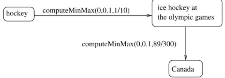
(this information is available in [43]), we present a previ-ously unpublished example that demonstrates how we can return semantically relevant documents based on informa-tion from Wikipedia. Consider Fig. 3. It describes that the word “hockey” appears in the title of the Wikipedia arti-cle about ice hockey in the Olympic Games and that the word “Canada” appears in this Wikipedia article 89 times. As a result, we can extract information about the relation-ship between the words “hockey” and “Canada”. Specif-ically, suppose that 10 Wikipedia titles contain the word “hockey”, where “Ice Hockey at the Olympic Games” is one of these pages. The edge between the nodes “hockey” and “Ice Hockey in the Olympic Games” will have a weight of computeMinMax(0,0.1,1/10), where the last parameter represents that the article is only one of 10 Wikipedia articles that have the word “hockey” in their title. Next, suppose that the word “Canada” appears 89 times in the Wikipedia article and that the size of the text that contains words that appear five times of more in the article is 300 words. Then we will draw the second edge that is shown in the figure with weight computeMinMax(0,0.1,89/300). The parameter 89/300 describes the contribution of the word “hockey” to the text that contains frequently accruing words. Note that for both edges the coefficient 0.1 is relatively low because the information in Wikipedia is not as reliable as the information in WordNet.
computeMinMax(0,0.1,1/10) hockey
computeMinMax(0,0.1,89/300) ice hockey at the olympic games
Canada
Fig. 3. Example part of a similarity graph that is created from Wikipedia.
Next, consider Fig. 4. The nodes in the graph represent the Wikipedia article on hockey and the word “Canada”. Suppose that the word “Canada” appears 10 times in the body of the article. If we assume that the size of the text in the Wikipedia article on Canada that consists of words that repeat five times or more is 45 words, then we will create the edge that is shown in the figure. The parameter 10/45describes the contribution of the word “Canada” to the text that contains frequently accruing words. Since this is the second path between the nodes with labels “hockey” and “Canada”, we need to aggregate the evidence from the two paths and get the number computeMinMax(0,0.1,1/10)∗computeMinMax(0,0.1,89/300) + computeMinMax(0,0.1,10/45) = 0.05. In other words, based on the presented Wikipedia evidence, we will consider documents that contain the word “Canada” when searching for documents about hockey. However, we will assign weight to these documents for the word “hockey” of only 0.05. Alternatively, documents that contain the word “hockey” will be assigned the full weight of 1 for the word “hockey”.
hockey
Canada
computeMinMax(0,0.1,10/45)
Fig. 4. Example part of a similarity graph that is created from Wikipedia.
IV. ADDING QUERIES AND DOCUMENTS TO THE
SIMILARITY GRAPH
Let us examine the first query of the Cranfield benchmark (see [6]): “What similarity laws must be obeyed when con-structing aeroelastic models of heated high speed aircraft?” After we remove all the noise words, we are left with 10 words. We are going to create a node for the query and draw an edge to each of the 10 word nodes – see Fig. 5. We will use term to refer to both a word form or a phrase that is a Wikipedia page title. In general, we consider all the terms in the query and try to match them against node labels in the graph. In the specific example, there are no Wikipedia pages that contain terms of two words or more from the query. If there were, then edge will be drawn to these nodes as well. The weight of each edge is equal to computeMinMax (0,1, ratio), where ratio is the number of times the term appears in the query divided by the total number of terms that are considered. As explained in the previous section, the computeMinMax function can be used to smoothen the result. In other words, we do not consider a term that appears twice in the query twice more important than a term that appears only once. The computeMinMax function makes the ratio of the two cases 1.3 instead of 2. As we will describe later in this section, the graph model can be used to implement the standard TF-IDF scoring function. If we follow this model, then the weight of each of the edges should be equal to the value of the ratio parameter. Note that multiplying the weights of the edges by a number will not affect the ranking of the query result. Here, we multiply by one because we assume that there is a 100% probability that the user will be interested in one of the terms in their query. Note as well that we give equal importance to all the terms in the query and we do not assume that the leading terms are more important. Of course, this model can be adjusted if the user specifies the importance of each term in the query using a numerical value.
Fig. 5 shows how the query is connected to the similarity graph. The weight of each edge is equal to
computeMinMax (0,1,1/10) = 0.3. If the query contains a word that is not part of the similarity graph (i.e., not in WordNet), then we will not draw an edge for this word. As an alternative example, if there is a Wikipedia page with title “high speed aircraft”, then a node with this label will exist in the similarity graph and we will draw an edge between the query and the node.
Next, let us consider the first document in the Cranfield benchmark. The word “propeller” appears once in the body of
√
∗(1+log2(numDocs
weight= tf ))2
docFreq+1
P p numDocs
score(q,d) = ( tf (tind)∗(1+log2(docFreq(t)+1))2) tinq aeroelastic Q1 aircraft speed heated models constructing obeyed laws similarity high
all edge weights: computeMinMax(0,1,0.1)
Fig. 5. Connecting the first query of the Cranfield benchmark to the similarity graph.
the article and it does not appear in its title. Suppose that the word also appears once in three other documents. Then we will create the subgraph that is shown in Fig. 6. In general, the weight of an edge from a term to a document that contains the term in the tile is equal to computeMinMax (0,0.8, ratio) and to a document that contains the term in the body –
computeMinMax (0,0.2,ratio). Here, ratiois the number of times the term appears in the title or body of the document, respectively, divided by the total number of occurrences in all documents. The reason behind these formulas is that we believe that documents that have a term from the query in their title are more likely to be relevant than documents that contain the term in the body of the document. To put it differently, the formula implies that there is an 80% chance that a user that is interested in a term will be also interested in one of the documents that contains the term in the title. Similarly, there is a 20% chance that the user will be interested in one of the documents that contains the term in its body.
computeMinMax(0,0.2,1/4) propeller
document 1
all edges:
Fig. 6. Connecting the word “propeller” with the documents.
Note that the formulas for computing the edge weights that connect documents and queries to the graph follows the TF-IDF model. When computing the value for the ratio parameter, we consider the number of times the term appears in the document (the term frequency) and divide by the number of times the term appears in all documents (the document frequency). In other words, we multiply the term frequency by the inverse of the document frequency. An alternative formula for calculating the weight of an edge between a term and a document is shown below. This formula is based on the way the ranking function is computed in the Apache Lucene system ([10]).
In the above formula, tf is the number of times the
term appears in the document, numDocs is the total number of documents, and docFreq is the number of documents in which the term appears. In order to be consistent with the previous way of computing the edge weights, we need to multiply the weights of edges that represent the containment of a term in the title of a document by 0.8 and the weights of edges that represent the containment of a term in the body of a document by 0.2. In the experimental section of this paper, we compare the two ways of connecting queries and documents to the graph.
Note that the main contribution of the paper is incorporating the similarity graph when returning relevant documents ranked based on their relevance to the input query. If we remove the similarity graph that is created from WordNet and Wikipedia, then we will only draw edges from the query to the words in the query and from the words in the query to the documents, which is equivalent to applying the TF-IDF model for ranked document retrieval. In other words, the paper proposes an extension the TF-IDF model by adding information about term similarity that can be extracted from WordNet and Wikipedia.
V. SCORING FUNCTIONS
First, let us examine the scoring function that is used by Apache Lucene ([10]), which is a popular software that contains a toolkit of routines for information retrieval. Given a document d and a query q, the scoring function is defined as follows.
In the function, tf (t in d) denotes the number of ap-pearances of the term t in the document d, numDocs refers to the total number of documents, and docFreq(t) refers to the number of documents in which the term t appears. This follows the TF-IDF formula because the second part of the formula is one way of computing the inverse document frequency. The scoring function can be multiplied by boosting and normalizing parameters, which are skipped because they are optional parameters and require user tuning.
Next, let us consider how the similarity graph can be used to compute the value of the scoring function. Recall that the weight of an edge in the similarity graph is used to represent the conditional probability that a user is interested in the destination concept given that they are interested in the source concept. We compute the directional similarity between two nodes using the following formula.
X
A→sC= PPt(C|A) (1)
Pt is a cycleless path from node A to node C
Y
PPt(C|A) = P(n2|n1) (2)
(n1,n2)is an edge in the path Pt
In the above formula, P(n2|n1)is used to denote the weight of the edge from the node n1 to the node n2. Informally, we compute the directional similarity between two nodes
d X 1 MAP(Q) = Precision(Ri) d i=1 1 |w1, w2|= 0.8∗min(α,w1→sw2)∗ α
#(relevant items retrieved)
Precision(Ri) =
#(retrieved items) in the graph as the sum of all the paths between the two
nodes, where we eliminate cycles from the paths. Each path provides evidence about the similarity between the terms that are represented by the two end nodes. We compute the similarity between two nodes along a path as the product of the weights of the edges along the path, which follows the Markov chain model. Since the weight of an edge along the path is almost always smaller than one (i.e., equal to one only in rear circumstances), the value of the conditional probability will decrease as the length of the path increases. This is a desirable behavior because a longer path provides less evidence about the semantic relationship between the two end nodes.
Note that the value of A→s C can be potentially greater than 1. Therefore, we will apply the following function for normalizing the relevance score between two internal nodes of the graph (i.e., nodes that do not represent queries or documents).
(3) In previous work (e.g., [44], [43]) we have shown that value of 0.1 for α produces data of good quality. Here, we will use this value. The function transforms the relevance score between two internal nodes into the range [0,0.8]. The value 0.8 guarantees that if we substitute a term in the query with a different term, then the new term will be weighted with value 0.8 or less. Using this new function, the relevance score between a query q and a document d is computed as follows, where w1 iterates over all nodes that can be reached by following an edge from q and w2 are nodes that have a direct edge to d.
P
relevance score(q,d) = P(w1|q)∗|w1→sw2|∗p(d|w2) w1,w2
In the above formula, for each value of w1 we restrict w2 to the 50 nodes that have the highest relevance score with w1. In other words, we consider up to 50 substitutions for every term in the query.
VI. EXPERIMENTAL RESULTS
The Cranfield benchmark ([6]) contains 1400 short docu-ments about the physics of aviation. Each document contains a title and a short body that is usually around 10 lines. As part the benchmark, 225 natural language queries were created. As part of the study, the documents and queries were examined by experts in the area and the documents that are relevant to each query were identified. The relevant documents were clustered in four groups. Highly relevant documents were given relevance score of 1, less relevant documents were given a relevance score of 2, even less relevant documents were given a relevance score of 3, while documents of minimum interest were given a relevance score of 4.
As Table I suggests, for each algorithm we ran four ex-periments. In the first experiment, we only considered the documents with relevance score of 1 to be relevant. In the second experiment, we only considered the documents with relevance scores of 1 and 2 to be relevant and so on. Each
Rel. 1 Rel. 1-2 Rel. 1-3 Rel. 1-4
Similarity Graph + our weights 0.29 0.29 0.30 0.35 Similarity Graph + Lucene weights 0.28 0.28 0.30 0.34 Lucene Algorithm 0.25 0.25 0.27 0.29 Lucene Algorithm + our weights 0.26 0.26 0.27 0.30 TABLE I
MAP VALUES FOR DIFFERENT ALGORITHMS AND DEGREES OF
RELEVANCE FOR THE CRANFIELD BENCHMARK.
of the experiments took about 10 minute to complete on a typical laptop with an Intel Core i7 processor and 4GB of main memory.
For each query, we computed the mean average precision score, which is also known as the MAP score. Consider the query Q. Let {Di}di=1 be the relevant documents. Let Ri be the set of documents that are retrieved by the algorithm until document Di is returned. Then the MAP score for the query Qis defined as the average precision of Ri over all values, or formally as follows.
(4) The precision for Ri is defined as the fraction of retrieved documents that are relevant, or formally as follows.
(5) Next, let us examine Table I in more details. The MAP score is the average MAP value over all 225 queries. The top algorithm is the algorithm that is described in the paper. As the table suggests, it produces higher value for the MAP metric than the Apache Lucene algorithm. The reason is that the later performs simple keywords matching and does not consider the semantic relationship between the terms in queries and documents. It is clear from the table that our algorithm produces especially good results when we consider documents with relevance score from 1 to 4 to be relevant. The reason is that our algorithm is strong at identifying documents that are weakly related with the input query. Alternatively, the Apache Lucene algorithm fails to discriminate between documents that do not contain the query words.
It is also worth noting that our edge weight functions for connecting the query and document nodes to the graph produce slightly higher values for the MAP score than the functions that are used in the Apache Lucene algorithm.
VII. CONCLUSION AND FUTURE RESEARCH
In two previous papers, we showed how to create a sim-ilarity graph that stores the degree of semantic relationship between terms ([44], [43]). In this paper we apply the semantic similarity graph to the problem of ranked document retrieval. Specifically, we enhanced the TF-IDF document retrieval algorithm with the similarity graph and presented an algorithm
that retrieves documents based on the similarity between the terms in the documents and the terms in the query. We experimentally validated the algorithm by showing that the similarity graph can contribute to achieving more relevant results than using the TF-IDF approach alone.
In the future, we plan to continue exploring new applications of the similarity graph. Incorporating the graph in a query answering system that uses an ontology and using the graph to cluster documents based on the meaning of the terms in them are two possible areas for future research.
REFERENCES
[1] A. A. Bernstein and E. Kaufmann. Gino - A Guided Input Natural Lan-guage Ontology Editor. Fifth International Semantic Web Conference, 2006.
[2] M. Agosti and F. Crestani. Automatic Authoring and Construction of Hypertext for Information Retrieval. ACM Multimedia Systems, 15(24), 1995.
[3] M. Agosti, F. Crestani, G. Gradenigo, and P. Mattiello. An Approach to Conceptual Modeling of IR Auxiliary Data. IEEE International Conference on Computer and Communications, 1990.
[4] C. Buckley and E. M. Voorhees. Evaluating evaluation measure stability.
Proceeding of ACM Special Interest Group on Information Retrieval, pages 33–40, 2000.
[5] P. Cimiano, P. Haase, and J. Heizmann. Porting Natural Language Interfaces between Domains – An Experimental User Study with the ORAKEL System. International Conference on Intelligent User Inter-faces, 2007.
[6] C. W. Cleverdon. The Significance of the Cranfield Tests on Index Languages. In Proceedings of Special Interest Group on Information Retrieval, pages 3–12, 1991.
[7] P. Cohen and R. Kjeldsen. Information Retrieval by Constrained Spreading Activation on Sematic Networks. Information Processing and Management, pages 255–268, 1987.
[8] F. Crestani. Application of Spreading Activation Techniques in Infor-mation Retrieval. Artificial Intelligence Review, 11(6):453–482, 1997. [9] Croft. User-specified Domain Knowledge for Document Retrieval.
Nineth Annual International ACM Conference on Research and Devel-opment in Information Retrieval, pages 201–206, 1986.
[10] D. Cutting. Apache Lucene. http://lucene.apache.org, 2014.
[11] S. Deerwester, S. T. Dumais, G. W. Furnas, T. K. Landauer, and R. Harshman. Indexing by Latent Semantic Analysis. Journal of the Society for Information Science, 41(6):391–407, 1990.
[12] C. Fox. Lexical Analysis and Stoplists. Information Retrieval: Data Structures and Algorithms, pages 102–130, 1992.
[13] W. Frakes. Stemming Algorithms. Information Retrieval: Data Struc-tures and Algorithms, pages 131–160, 1992.
[14] T. Gruber. Collective knowledge systems: Where the social web meets the semantic. Web Journal of Web Semantics, 2008.
[15] R. V. Guha, R. McCool, and E. Miller. Semantic Search. Twelfth International World Wide Web Conference (WWW 2003), pages 700– 709, 2003.
[16] A. M. Harbourt, E. Syed, W. T. Hole, and L. C. Kingsland. The Ranking Algorithm of the Coach Browser for the UMLS Metathesaurus.
Seventeenth Annual Symposium on Computer Applications in Medical Care, pages 720–724, 1993.
[17] W. R. Hersh and R. A. Greenes. SAPHIRE An Information Retrieval System Featuring Concept Matching, Automatic Indexing, Probabilistic Retrieval, and Hierarchical Relationships. Computers and Biomedical Research, pages 410–425, 1990.
[18] W. R. Hersh, D. D. Hickam, and T. J. Leone. Words, Concepts, or Both: Optimal Indexing Units for Automated Information Retrieval. Sixteenth Annual Symposium on Computer Applications in Medical Care, pages 644–648, 1992.
[19] E. H. Hovy, L. Gerber, U. Hermjakob, M. Junk, and C. Y. Lin. Question Answering in Webclopedia. TREC-9 Conference, 2000.
[20] K. Jarvelin, J. Keklinen, and T. Niemi. ExpansionTool: Concept-based Query Expansion and Construction. Springer Netherlands, pages 231– 255, 2001.
[21] G. Jeh and J. Widom. SimRank: A Measure of Structural-context Similarity. Proceedings of the Eight ACM SIGKDD International Conference on Knowledge Discovery and Data Mining, pages 538–543, 2002.
[22] K. Jones. ”a statistical interpretation of term specificity and its applica-tion in retrieval”. Journal of Documentation, 28(1):11–21, 1972. [23] S. Jones. Thesaurus Data Model for an Intelligent Retrieval System.
Journal of Information Science, 19(1):167–178, 1993.
[24] A. Kiryakov, B. Popov, I. Terziev, D. Manov, and D. Ognyanoff. Se-mantic Annotation, Indexing, and Retrieval. Journal of Web Semantics, 2(1):49–79, 2004.
[25] R. Knappe, H. Bulskov, and T. Andreasen. Similarity Graphs. Fourteenth International Symposium on Foundations of Intelligent Systems, 2003. [26] T. K. Landauer, P. Foltz, and D. Laham. Introduction to Latent Semantic
Analysis. Discourse Processes, pages 259–284, 1998.
[27] V. Lopez, M. Fernndez, E. Motta, and N. Stieler. PowerAqua: Supporting Users in Querying and Exploring the Semantic Web Content. Semantic Web Interoperability, Usability, Applicability an IOS Press Journal, 2010.
[28] V. Lopez, M. Pasin, and E. Motta. AquaLog: An Ontology-portable Question Answering System for the Semantic Web. European Semantic Web Conference, pages 546–562, 2005.
[29] V. Lopez, M. Sabou, and E. Motta. PowerMap: Mapping the Real Semantic Web on the Fly. Fifth International Semantic Web Conference (ISWC2006), 2006.
[30] M.F.Porter. An Algorithm for Suffix Stripping. Readings in Information Retrieval, pages 313–316, 1997.
[31] G. A. Miller. WordNet: A Lexical Database for English. Communica-tions of the ACM, 38(11):39–41, 1995.
[32] D. Moldovan, S. Harabagiu, M. Pasca, R. Mihalcea, R. Goodrum, and R. Girju. LASSO: A Tool for Surfing the Answer Net. Text Retrieval Conference (TREC-8), 1999.
[33] C. Paice. A thesaural model of information retrieval. Information Processing and Management, 27(1):433–447, 1991.
[34] B. Popov, A. Kiryakov, D. D. Ognyanoff, D. Manov, and A. Kirilov. KIM A Semantic Platform for Information Extraction and Retrieval.
Journal of Natural Language Engineering, 10(3):375–392, 2004. [35] L. Rau. Knowledge Organization and Access in a Conceptual
Informa-tion System. Information Processing and Management, 23(4):269–283, 1987.
[36] C. Rocha, D. Schwabe, and M. Aragao. A Hybrid Approach for Searching in the Semantic Web. Thirteenth International World Wide Web Conference (WWW 2004), pages 374–383, 2004.
[37] S. S. Luke, L. Spector, and D. Rager. Ontology-Based Knowledge Discovery on the World Wide Web. Internet-Based Information Systems: Papers from the AAAI Workshop, pages 96–102, 1996.
[38] M. Sanderson. Word Sense Disambiguation and Information Retrieval.
Seventeenth annual international ACM SIGIR conference on Research and development in information retrieval, 1994.
[39] P. Shoval. Expert consultation system for a retrieval database with semantic network of concepts. Fourth Annual International ACM SIGIR Conference on Information Storage and Retrieval: Theoretical Issues in Information Retrieval, pages 145–149, 1981.
[40] Simone Paolo Ponzetto and Michael Strube. Deriving a Large Scale Taxonomy from Wikipedia. 22nd International Conference on Artificial Intelligence, 2007.
[41] E. Sirin and B. Parsia. SPARQL-DL: SPARQL Query for OWL-DL.
3rd OWL: Experiences and Directions Workshop (OWLED), 2007. [42] K. Srihari, W. Li, and X. Li. Information Extraction Supported Question
Answering. In Advances in Open Domain Question Answering, 2004. [43] L. Stanchev. Creating a Phrase Similarity Graph from Wikipedia. Eight
IEEE International Conference on Semantic Computing, 2014. [44] L. Stanchev. Creating a Similarity Graph from WordNet. Fourth
International Conference on Web Intelligence, Mining and Semantics, 2014.
[45] N. Stojanovic. On Analyzing Query Ambiguity for Query Refinement: The Librarian Agent Approach. Twenty Second International Conference on Conceptual Modeling, pages 490–505, 2003.
[46] The World Wide Web Consortium. OWL Web Ontology Language Guide. http://www.w3.org/TR/owl-guide/, 2014.
[47] Y. Yang and C. G.Chute. Words or Concepts: The Features of Indexing Units and their Optimal use in Information Retrieval. Seventeenth Annual Symposium on Computer Applications in Medical Care, pages 685–68, 1993.