Proximal Splitting Methods in
Nonsmooth Convex Optimization
An der Fakultät für Mathematik der Technischen Universität Chemnitz eingereichte
D I S S E R T A T I O N
zur Erlangung des akademischen Grades
Doctor rerum naturalium
(Dr. rer. nat.)
Vorgelegt von
Dipl.-Math. oec. Christopher Hendrich
Fachbereich für Angewandte Mathematik (Approximationstheorie)
Gefördert durch ein Landesstipendium des Freistaates Sachsen
Gutachter: Prof. Dr. Radu Ioan Boţ (Betreuer) Prof. Dr. Heinz H. Bauschke
Prof. Dr. Gabriele Steidl
Tag der Einreichung: 28. April 2014 Tag der Verteidigung: 17. Juli 2014
Christopher Hendrich
Proximal Splitting Methods in Nonsmooth Convex Optimization
Dissertation, 142 pages, Technische Universität Chemnitz, Department of Mathe-matics, 2014
Report
This thesis is concerned with the development of novel numerical methods for solving nondifferentiable convex optimization problems in real Hilbert spaces and with the investigation of their asymptotic behavior. To this end, we are also making use of monotone operator theory as some of the provided algorithms are originally designed to solve monotone inclusion problems.
After introducing basic notations and preliminary results in convex analysis, we derive two numerical methods based on different smoothing strategies for solving nondifferentiable convex optimization problems. The first approach, known as the double smoothing technique, solves the optimization problem with some given a priori accuracy by applying two regularizations to its conjugate dual problem. A special fast gradient method then solves the regularized dual problem such that an approximate primal solution can be reconstructed from it. The second approach affects the primal optimization problem directly by applying a single regularization to it and is capable of using variable smoothing parameters which lead to a more accurate approximation of the original problem as the iteration counter increases.
We then derive and investigate different primal-dual methods in real Hilbert spaces. In general, one considerable advantage of primal-dual algorithms is that they are providing a complete splitting philosophy in that the resolvents, which arise in the iterative process, are only taken separately from each maximally monotone operator occurring in the problem description. We firstly analyze the forward-backward-forward algorithm of Combettes and Pesquet in terms of its convergence rate for the objective of a nondifferentiable convex optimization problem. Additionally, we propose accelerations of this method under the additional assumption that certain monotone operators occurring in the problem formulation are strongly monotone. Subsequently, we derive two Douglas–Rachford type primal-dual methods for solving monotone inclusion problems involving finite sums of linearly composed parallel sum type monotone operators. To prove their asymptotic convergence, we use a common product Hilbert space strategy by reformulating the corresponding inclusion problem reasonably such that the Douglas–Rachford algorithm can be applied to it. Finally, we propose two primal-dual algorithms relying on forward-backward and forward-backward-forward approaches for solving monotone inclusion problems involving parallel sums of linearly composed monotone operators.
The last part of this thesis deals with different numerical experiments where we intend to compare our methods against algorithms from the literature. The problems which arise in this part are manifold and they reflect the importance of this field of research as convex optimization problems appear in lots of applications of interest.
primal-dual algorithm, smoothing technique, monotone inclusions, conjugate duality, convex optimization, nonsmooth opimization, proximal point mapping, resolvent, projection, imaging, location problems, machine learning, portfolio optimization, clustering
It is a pleasure for me to thank the people who supported me during my research. This thesis would not have been possible without the assistance and advice of Prof. Dr. Radu Ioan Boţ. I want to thank him for proposing this topic to me, for his commitment, and for being available for countless discussions. I also want to express my gratitude to Prof. Dr. Gert Wanka for the continuous support during my doctoral study. Many thanks go to our research group, our guests, and my office colleagues for the warmhearted and friendly atmosphere at the department.
I would like to thank Prof. Dr. Heinz H. Bauschke and Prof. Dr. Gabriele Steidl for their contribution in reviewing this thesis and for their valuable remarks and comments which improved the quality of this thesis.
I am grateful to the Free State of Saxony for the financial support of my research by granting me with a graduate fellowship.
I am also grateful to the Department of Mathematics, Technische Universität Chemnitz, for providing me a good research environment.
1 Introduction 11 1.1 A description of the content . . . 33 1.2 Notation and preliminaries . . . 55
2 Smoothing techniques in convex optimization 1313
2.1 Double Smoothing Technique . . . 1313 2.1.1 Problem description . . . 1414 2.1.2 First and second smoothing . . . 1616 2.1.3 An appropriate fast gradient method . . . 2121 2.1.4 Convergence of θ(pk) to θ(p∗) . . . 2222
2.1.5 Convergence of k∇θρ,µ(pk)k to 0 . . . 2424
2.1.6 How to construct an approximately primal optimal solution . . . 2626 2.1.7 Existence of an optimal solution . . . 2727 2.1.8 Improving the convergence rates . . . 2727 2.2 Variable Smoothing . . . 3232 2.2.1 Problem description . . . 3333 2.2.2 The smoothing of the problem (P) . . . 3434 2.2.3 The variable and the constant smoothing algorithm . . . 3535 2.2.4 The case whenf is differentiable with Lipschitz continuous gradient 4141 2.2.5 The optimization problem with the sum of more than two
func-tions in the objective . . . 4444
3 Primal-dual algorithms for inclusion problems 4747
3.1 Convergence analysis of a forward-backward-forward method . . . 4747 3.1.1 Problem description . . . 4848 3.1.2 Convergence estimates for convex minimization problems . . . . 5050 3.1.3 Zeros of sums of monotone operators . . . 5656 3.2 A Douglas–Rachford type primal-dual method . . . 6464 3.2.1 Problem description . . . 6565 3.2.2 A first primal-dual algorithm . . . 6666 3.2.3 A second primal-dual algorithm . . . 7373 3.2.4 Application to convex minimization problems . . . 7878 3.3 Solving inclusions with parallel sums of linearly composed monotone
operators . . . 8282 3.3.1 Problem description . . . 8383 3.3.2 An algorithm of forward-backward type . . . 8585 3.3.3 An algorithm of forward-backward-forward type . . . 9191 3.3.4 Application to convex minimization . . . 9494
4.1.1 TV-based image denoising . . . 101101 4.1.2 TV-based image denoising involving higher-order derivatives . . . 104104 4.1.3 TV-based image deblurring . . . 108108 4.1.4 TV-based image inpainting . . . 110110 4.2 Kernel based machine learning . . . 110110 4.3 The generalized Heron problem . . . 113113 4.4 Portfolio optimization under different risk measures . . . 115115 4.5 Clustering . . . 121121
Theses 124124
Symbols and notation 128128
Bibliography 131131
Index 138138
Curriculum Vitae 141141
2.1 Illustration of the sum problem appearing in Example 2.112.11 . . . 4141 4.1 An image denoising problem on the lichtenstein test image . . . 103103 4.2 An image denoising problem with first- and second-order total variation
functionals on the lichtenstein test image . . . 106106 4.3 An ISNR value comparison for the problem with first- and second-order
total variation functionals . . . 107107 4.4 An image deblurring problem on the cameraman test image . . . 108108 4.5 Performance evaluation of an image deblurring problem . . . 109109 4.6 An image inpainting problem on the fruits test image . . . 110110 4.7 Sample data for the kernel-based classification problem . . . 111111 4.8 The generalized Heron problem in two dimensions with numerical results114114 4.9 The generalized Heron problem in three dimensions with numerical
results . . . 115115 4.10 The clustering problem of two interlocking half moons showing the
correct affiliations . . . 121121
4.1 Performance evaluation for the image denoising problem . . . 104104 4.2 Misclassification rate in percentage for different model parameters in
the classification problem . . . 112112 4.3 Performance evaluation for the classification problem . . . 113113 4.4 Performance evaluation for the portfolio optimization problem . . . . 120120 4.5 Performance evaluation for the clustering problem . . . 122122
1
Introduction
In the last couple of years, a special attention within applied mathematics was given on the development of numerical methods for solving structured convex optimization problems having nonsmooth terms in their objectives. This effort is motivated by numerous applications, for example in fields like signal and image processing, portfolio optimization, cluster analysis, and location theory, this enumeration being by far not complete. When characterizing optimality, the convexity allows to make use of powerful results in convex analysis, separation theorems and the (Fenchel) conjugate theory here included. Literature on this topic can be found in [1111,2222,3030,6767,8282,119119,127127] and in the seminal work by Rockafellar from 1970 (cf. [106106]).
By considering the active and competitive branch of research for solving convex optimization problems numerically, this thesis is concerned with the development of efficient splitting algorithms for approximating optimal solutions of nondifferentiable convex optimization problems, and, more generally, with the solving of monotone inclusions in real Hilbert spaces. To this end, we propose and investigate a number of numerical methods relying on first-order information which either belong to the class of smoothing or primal-dual algorithms.
The principal character of smoothing algorithms is to apply appropriate smoothing techniques as the ones discussed in [9999–101101] to the problem under investigation, in order to approximate nondifferentiable convex functions by continuously differentiable ones. The resulting problem is then solved via some of the accelerated gradient methods by Nesterov (see [9797, 9898, 100100]). In fact, we propose and discuss two different smoothing algorithms, one of them being able to reduce the smoothing impact as the iteration counter increases, which, in contrast to the approach involving constant smoothing parameters, leads to a more accurate approximation of the original objective function. Then, instead of determining gradients, the calculation of proximal point mappings of the functions in the objective arises in the numerical scheme. However, it is worth to mention that the proximal point mappings are applied to the functions in the objective separately and that bounded linear operators occuing in the problem formulation (respectively their adjoints) are evaluated explicitly via forward steps. This uncovers an important distinction when compared with the majority of numerical methods relying on augmented Lagrangian (cf. [11,4242,6868,7474,7777,8181,124124–126126]) and iterative tresholding (cf. [1515, 1616, 1919, 5656, 6262]) approaches, themselves only featuring
an unsatisfactory splitting behavior.
Primal-dual algorithms, on the other hand, build the second important class of numerical methods that we address in this thesis. These methods are predominantly designed to solve primal-dual systems of monotone inclusion problems where the dual inclusion is formulated in the sense of Attouch–Théra (cf. [77]). They can, however, give rise to the solving of convex optimization problems by taking into account appropriate qualification conditions. In general, primal-dual algorithms are more attractive from a conceptual point of view than those relying on smoothing strategies. This is justified by the property of primal-dual methods to solve systems of first-order optimality conditions, hence they solve the original optimization problem rather than a perturbed version of it. In addition, primal-dual algorithms provide convergence statements for the sequences of iterates whereas smoothing algorithms only guarantee convergence with respect to the function values.
To the oldest and most popular methods for solving monotone inclusion problems belong the proximal point algorithm by Martinet in [9292], which was further generalized by Rockafellar in [109109], and the Douglas–Rachford splitting algorithm (cf. [6464]). The latter was, together with the related Peaceman–Rachford algorithm (cf. [104104]), shown to be applicable to evolution equations in [8888] and also recovers, in convex optimization, the popular alternating direction method of multipliers (ADMM, cf. [6868, 7575]) when applied to the conjugate dual problem as is discussed in [7676]. In general, the Douglas–Rachford algorithm is designed to find a point in the set of zeros with respect to the sum of two maximally monotone operators as is detailed in Problem 1.11.1 below.
Problem 1.1Let H be a real Hilbert space and let A, B be maximally monotone operators mapping from H to 2H. The problem is to
find x∈ H such that 0 ∈Ax+Bx. (1.1) This method, whose roots go back to the year 1956, processes the resolvents of the maximally monotone operators occurring in Problem 1.11.1 separately in each iteration. The resolvent of a maximally monotone operator corresponds to a proximal point mapping when applied to the subdifferential of a proper, convex, and lower semicontinuous function (itself being a maximally monotone operator, cf. Rockafellar [107107]). Demonstrating the importance of operator splitting, we can consider the situation when the sum A+B in Problem 1.11.1 is maximally monotone. Then, the proximal point algorithm can also be applied to it, but it requires the determination of the resolvent ofA+B which may be very hard in general, even in the case when the resolvents ofA and B have a simple representation taken separately.
The monotone inclusion in Problem 1.11.1 corresponds, under certain qualification conditions, to the solving of a convex optimization problem involving the sum of two proper, convex, and lower semicontinuous functions. However, many optimization problems appearing in real-world applications take more sophisticated representations. As this gives rise via convex duality and optimality statements to the solving of monotone inclusions involving mixtures of linear composite, single-valued Lipschitzian, and/or cocoercive and parallel sum type operators, the question is to find easily implementable schemes for these more intricate formulations. Taking this into account, one considerable aim is to avoid asking for the resolvents of sums, parallel
sums, and compositions with bounded linear operators, for which in general no exact formulae exist. On the other hand, one aims to include the single-valued operators via forward evaluations into the iterative process of the algorithm as these steps are in general easier to identify than backward evaluations which require the calculation of resolvents.
As the three fundamental splitting approaches in the shape of Tseng’s forward-backward-forward algorithm (cf. [121121]), the forward-backward algorithm (cf. [8888,103103]), and the Douglas–Rachford algorithm (cf. [6464]) showed to have substantial limitations in this context, first fruitful ideas were developed by Chambolle and Pock in [4848] for solving convex optimization problems and by Combettes and Briceño-Arias in [4343] for solving monotone inclusions. There, in addition to Problem 1.11.1, the authors also consider some linear compositions within the problem formulation and derive numerical schemes in the sense of an appropriate splitting. The ideas in [4343] were further extended by Combettes and Pesquet in [5858] to a monotone inclusion problem involving a single-valued monotone Lipschitzian operator and arbitrary finite sums of linearly composed parallel sum type monotone operators. By reformulating this problem in an appropriate Hilbert product space, the authors reduce the monotone inclusion to the one of finding a zero in the sum of a maximally monotone with a monotone Lipschitzian operator. The latter is then solved via some variant of Tseng’s forward-backward-forward algorithm featuring a tolerance towards errors in the shape of summable sequences, which may arise within the implementation. This method also allows to access the single-valued Lipschitzian operators explicitly via forward steps and it is capable of processing maximally monotone and bounded linear operators separately whenever they arise in the shape of precompositions within the problem description.
This concept was further employed by V˜u in [122122] in order to solve systems of monotone inclusions with comparable structural complexity. There, instead of assuming monotone Lipschitzian operators, attention is given to monotone cocoercive operators. As a consequence, instead of making use of Tseng’s splitting algorithm, an error sensitive forward-backward method is used, which, however, relies on the use of considerably different technical arguments. If we return to the popular primal-dual method due to Chambolle and Pock described and analyzed in [4848, Algorithm 1] and its extension proposed by Condat in [6060], it can be shown that these methods are particular instances of V˜u’s algorithm.
In addition to the important paper by Combettes in [5353], which discusses the solving of monotone inclusions in a general framework via nonexpansive averaged operators, other recently introduced splitting algorithms for solving monotone inclusions can be found in [1212, 1717, 2323, 2525, 5454, 6666, 105105, 128128] and for the inertial case in [22, 33, 2424, 2727], while coupled monotone inclusions are analyzed in [55, 66, 2929, 4444, 5555, 123123] and convergence rate estimates are provided in [2626, 8686]. By taking into account constrained convex optimization problems, first fruitful ideas involving easily implementable epigraphical projection approaches are provided in [5151, 8080].
1.1 A description of the content
In the remainder of this chapter we introduce our notation and preliminary results in convex analysis.
In Chapter 22, we propose two different smoothing algorithms for solving nondiffer-entiable convex optimization problems. These two approaches rely, on the one hand, on our articles [3434, 3535] for the so-called double smoothing algorithm including its acceleration strategies, and, on the other hand, on the article [4040] for the so-called variable smoothing algorithm. Both algorithms share similarities as they make use of the concept of the Moreau envelope in order to approximate nondifferentiable convex objectives by continuously differentiable ones. Therefore, instead of involving gradient or subdifferential evaluations, these methods rely on the use of the proxim-ity operator. However, the two approaches are completely different to each other in view of the technical assumptions, the smoothing strategies, the fast gradient methods involved, the rates of convergence for the primal objective function, and the reconstruction of approximate primal solutions.
In Chapter 33, we investigate a number of primal-dual algorithms for solving structured monotone inclusion problems in real Hilbert spaces. This technique allows it to process the functions within the objectives separately via their resolvents (resp. proximal point mappings) without being obliged to apply smoothing strategies as in Chapter 22 which may distort the underlying optimization problem by approximating it via some continuously differentiable one. Additionally, primal-dual algorithms are well-suited to solve highly structured monotone inclusion problems as they are able to perform a complete splitting, explicit evaluations of bounded linear operators or their adjoints present in the problem formulation here included. We firstly analyze the forward-backward-forward algorithm of Combettes and Pesquet (cf. [5858]), as we did in our article [3939], in terms of its convergence rate for the objective of a nondifferentiable convex optimization problem. Subsequently, we propose accelerations of this method under the additional assumption that certain monotone operators occurring in the problem formulation are strongly monotone. The second section in this chapter is concerned with the solving of structured monotone inclusions via some Douglas– Rachford type primal-dual method, a novel approach which was subject to our article in [3838]. Finally, the last section in Chapter 33is devoted to our article in [3737] where we derive two different primal-dual algorithms for solving monotone inclusion problems involving parallel sums of linearly composed monotone operators.
In Chapter 44, we analyze the numerical performance of the methods established in Chapter 22and Chapter 33 by solving a range of nondifferentiable convex optimization problems coming from different areas of optimization. The first numerical experiments are applied to image processing problems, themselves representing a broad class of problems inclosing those in the fields of image denoising, deblurring and inpainting which are the ones discussed in this thesis. Thereafter, by making use of the theory of support vector machines, we solve an image classification problem where handwritten digits are classified by their corresponding number. Additionally, we solve the generalized Heron problem which can be seen as a generalized location problem where one minimizes the sum of distances to closed convex sets subject to a hard constraint on the optimal solution. Based on our article in [3636], we also demonstrate the applicability of primal-dual methods to portfolio optimization problems where one minimizes a convex risk functional (being associated with the so-called Optimized Certainty Equivalent) subject to a constraint on the expected return of the portfolio. Finally, our last numerical example is concerned with the solving of a problem which arises in clustering.
1.2 Notation and preliminaries
This section collects the most important notations, definitions and preliminary results which are used throughout this thesis. Appropriate literature on this topic can be found in [1111, 2222, 3030, 8282, 106106, 127127] and the references therein.
In the following, we are considering real Hilbert spaces H which are endowed with the inner product h·,·i and associated norm k·k= qh·,·i. When for i = 1, . . . , m, the real Hilbert spacesHi are endowed with inner producth·,·iHi and norm k·kHi =
q
h·,·iH
i, we denote by
H=H1⊕. . .⊕ Hm
theirHilbert direct sum. Forv = (v1, . . . , vm), q= (q1, . . . , qm)∈H, this real Hilbert
space is endowed with inner product and associated norm, respectively defined via
hv,qiH= m X i=1 hvi, qiiHi and kvkH= v u u t m X i=1 kvik2Hi. (1.2)
Note thatHcan be equivalently written as H= H1×. . .× Hm with scalar product
and norm defined via (1.21.2). By *and →we denote weak andstrong convergence, respectively. The Cauchy–Schwarz inequality, which follows next, plays a central role in all of mathematics.
Fact 1.2 (Cauchy–Schwarz inequality) Let x and y be in H. Then it holds
|hx, yi| ≤ kxkkyk. (1.3) The above inequality is fulfilled as equality if and only if there exists α ∈R such that x=αy ory=αx.
By N, we denote the set of natural numbers {1,2, . . .}, by R the set of real numbers, and by R+ the set ofpositive real numbers. We shall also use the set of
strictly positive real numbers denoted byR++=R+\{0} and the extended real line
R = R∪ {±∞}. By Rn, n ∈ N, we denote the n-dimensional Euclidean space
and we let 1n be the vector in Rn with all entries equal to 1. By B
H ⊆ H and
B(x, r) ⊆ H, we denote the closed unit ball in H and the closed ball centered at
x∈ H with radiusr ∈R++, respectively.
In the sequel we write min and max instead of inf and sup when the infimum or
supremum is attained, respectively. By arg min, we denote the set of minimizers
(oroptimal solutions) to a scalar optimization problem. For a primal optimization problem (P), we denote by v(P) its optimal objective value. For the associated dual optimization problem (D), the notationv(D) has a similar meaning. Having a primal-dual pair of optimization problems, then weak duality is fulfilled, if v(P) ≥ v(D) holds. On the other hand, we say thatstrong duality holds, when v(P) = v(D) and (D) has an optimal solution.
Having two nonempty sets C and D in H, their Minkowski sum is defined as
set λC = {λc : c ∈ C}, and let C⊥ = {x ∈ H : hx, yi = 0 ∀y ∈ C} be the
orthogonal complement of C. A nonempty set K ⊆ H is said to be a cone, if
λK ⊆ K for all λ ∈ R+ while the normal cone of a set C ⊆ H is defined as
NC(x) ={p∈ H:hp, y−xi ≤0 ∀y ∈C} for arbitrary x∈C, and being the empty
set for x6∈C. Theaffine hull of the set C⊆ H is nothing else than affC= n X i=1 λixi :n∈N, xi ∈C, λi ∈R, i= 1, . . . , n, n X i=1 λi = 1 .
We say thatC ⊆ H is convex, if
λC+ (1−λ)C ⊆C for all λ∈[0,1].
Let C ⊆ H be convex. By clC, intC, riC, and sqriC, we denote the closure, the
interior, therelative interior, and the strong quasi-relative interior of the convex set
C, where the latter is defined as sqriC =
x∈C : cone(C−x) is a closed linear subspace
.
In finite dimensional spaces, one has sqriC = riC, which is the interior ofC relative to its affine hull.
For a linear operator L:H → G, the operator L∗ :G → Hdenotes the adjoint op-erator ofLand fulfills the relation hL∗y, xi=hy, Lxifor all x∈ Hand ally ∈ G. By kerL={x∈ H:Lx= 0}andkLk, we denote the kernel ofLand its operator norm, respectively. We call the linear operatorL bounded (orcontinuous), ifkLk<+∞. For a given matrix A∈Rm×n,m, n∈N, the matrix AT is thetranspose of A.
Convex functions
For D ⊆ R, we say that the function f : D → R is increasing on D, if for every
a, b∈D such that a > b, we have f(a)≥f(b). On the other hand, we call f strictly increasing on D, if this inequality is fulfilled as strict inequality, i. e., f(a) > f(b). Consider the function f :H →R. By domf := {x∈ H:f(x)<+∞}, we denote itseffective domain and call f proper, if domf 6=∅ andf(x)>−∞ for all x∈ H. The set epif = {(x, r) ∈ H ×R : f(x) ≤ r} is called the epigraph of f. In the following, we introduce convex functions.
Definition 1.3 (Convex function) Let f : X → R be a given function and X a nonempty convex set inH. The function f is said to be convex onX, if
f(λx1+ (1−λ)x2)≤λf(x1) + (1−λ)f(x2)
for all x1, x2 ∈X and for all λ∈(0,1). The function f is calledstrictly convex on
X, if the above inequality is fulfilled as a strict inequality for each distinct x1 and
x2 in X and for each λ∈(0,1). The function f :X →Ris called concave (strictly concave) on X, if−f is convex (strictly convex) on X. An even stronger property is the existence of some γ ∈R++ such that
f(λx1+ (1−λ)x2) +
γ
2λ(1−λ)kx1−x2k 2 ≤
λf(x1) + (1−λ)f(x2)
for eachx1, x2 ∈X and for each λ∈(0,1). In this case, the function f is said to be
By taking into account the conventions (+∞) + (−∞) = +∞, 0·(+∞) = +∞ and 0·(−∞) = 0 (cf. [127127, p. 39]), the definition of convexity can be extended to functions ˜f :H →R mapping to the extended real line. We say that ˜f is convex, if for all x1, x2 ∈ H and for allλ∈[0,1]
˜
f(λx1+ (1−λ)x2)≤λf˜(x1) + (1−λ) ˜f(x2).
Therefore, the functionf :H →R is convex on the nonempty, convex set X ⊆ H, if and only if the function ˜f : H → R, ˜f(x) = f(x) for x ∈ X, and ˜f(x) = +∞, otherwise, is convex. Moreover, an important connection between functions and epigraphs is that the convexity of ˜f implies the convexity of epi ˜f and vice versa, as can be found in [2222, 3030, 106106, 127127].
We callf lower semicontinuous atx∈ H, if lim infy→xf(y)≥f(x). Moreover, the
functionf is called lower semicontinuous, if this holds for all x∈ H, or, equivalently, if epif is closed. An important class of functions is considered by the set Γ(H), which is defined as
Γ(H) :={f :H →R:f is proper, convex, and lower semicontinuous}. (1.4) Properness, convexity, and lower semicontinuity are our standard assumptions for the functions occurring in the optimization problems within this thesis.
The following definition of conjugate functions, which goes back to Fenchel (cf. [6969, 7070]), plays a central role in convex analysis.
Definition 1.4 (Conjugate function) Letf :H →R be a given function. Then the
(Fenchel) conjugate function off isf∗ :H →R,
f∗(p) = sup
x∈H
{hp, xi −f(x)} ∀p∈ H. (1.5) If conjugation is applied to f∗, we obtain f∗∗ := (f∗)∗ and call it the biconjugate
of f. The conjugate function f∗ of some arbitrary (not necessarily convex or lower semicontinuous) functionf :H →Ris always convex and lower semicontinuous and it holds the so-called Young–Fenchel inequality, i. e.,
f(x) +f∗(p)≥ hp, xi ∀x, p∈ H.
One of the most important theorems in conjugate duality is the Fenchel–Moreau Theorem.
Theorem 1.5 (Fenchel–Moreau) Let f ∈ Γ(H). Then the conjugate function f∗ is proper, convex, and lower semicontinuous andf∗∗=f.
Another fundamental instrument in convex analysis is the (convex) subdifferential.
Definition 1.6 (Convex subdifferential) Let f : H → R and x ∈ H be such that
f(x)∈R. An element p∈ H is called a subgradient of the function f at x, if
The set of all subgradients of the function f at xis denoted by ∂f(x) and is called the (convex) subdifferential of f atx. The subdifferential of f atx is considered to be empty, if f(x)∈ {±∞}. We say that f is subdifferentiable at x, if∂f(x)6=∅.
By taking into account convex functions, the subdifferential replaces the gradient in a more general sense by gathering similar properties. Therefore, the importance of the subdifferential is pointed out by the fact that functions in this work are generally considered to be convex and nondifferentiable. One also has the equivalent characterization
p∈∂f(x)⇔f(x) +f∗(p) = hp, xi,
i. e., for p, x∈ H fulfilling p∈ ∂f(x), the Young–Fenchel inequality is fulfilled as equality and vice versa.
A fundamental result in view of convex optimization is the following theorem which is known as Fermat’s rule.
Theorem 1.7 (Fermat’s rule) Let f :H → Rbe proper. Then
arg minf ={x∈ H : 0∈∂f(x)}.
The next definition concerns the notation of infimal convolutions.
Definition 1.8 (Infimal convolution) Having two proper functions f, g : H → R, their infimal convolution is defined by
fg :H →R, (fg)(x) = inf
y∈H{f(y) +g(x−y)} ∀x∈ H. (1.7) The infimal convolution in Definition 1.81.8 is a convex function when f and g are convex, while, forf, g∈Γ(H), the functionfg is not necessarily in Γ(H). However, whenever the condition (cf. [1111, 2222, 4545, 8585])
0∈sqri(domf∗ −domg∗) (1.8)
is fulfilled, one has fg ∈ Γ(H) and the infimal convolution is exact, i. e., the infimum in (1.71.7) is attained for all x∈ H. For other conditions guaranteeing (1.81.8), we refer the reader to [1111, Proposition 15.7].
Next, we introduce the notation of the Moreau envelope, which plays a central role in the development of our smoothing algorithms in Chapter 22.
Definition 1.9 (Moreau envelope) The Moreau envelope of parameter γ ∈ R++ of
f ∈Γ(H) is the function γf :H →R defined as
γf(x) := f 1 2γ k·k 2 (x) = inf y∈H ( f(y) + 1 2γkx−yk 2 ) ∀x∈ H. (1.9)
On the other hand, the proximal point mapping, which is closely connected with the Moreau envelope, plays a key role in smoothing and primal-dual algorithms.
Definition 1.10(Proximal point) Let f ∈Γ(H), γ ∈ R++, and x ∈ H. We denote by Proxγf(x) the proximal point (also called proximal point mapping) of γf at x,
representing the unique optimal solution of the minimization problem in (1.91.9), i. e., Proxγf(x) = arg min
y∈H
γf(y) + 1
2ky−xk
2. (1.10)
Notice that Proxγf : H → H is single-valued and firmly nonexpansive (cf. [1111,
Proposition 12.27]), i. e., it holds
kProxγf(x)−Proxγf(y)k2+k(x−Proxγf(x))−(y−Proxγf(y))k2 ≤ kx−yk2 (1.11)
for allx, y ∈ H. Therefore, the proximal point mapping is also Lipschitz continuous with Lipschitz constant equal to 1. For a large class of functions arising in different fields of applications, the proximal point mappings are given by exact formulae (cf. [5757, 5959]). We additionally have (cf. [1111, Theorem 14.3 (i)])
γf(x) + γ1f∗x γ = kxk 2 2γ ∀x∈ H, (1.12)
and the extended Moreau’s decomposition formula (cf. [1111, Theorem 14.3 (ii)]) Proxγf(x) +γProx1 γf ∗ x γ =x ∀x∈ H. (1.13)
The function γf is (Fréchet) differentiable on H and its gradient ∇(γf) :H → H
fulfills (cf. [1111, Proposition 12.29]) ∇(γf)(x) = 1
γ(x−Proxγf(x))∀x∈ H, (1.14)
being in the light of (1.111.11) γ−1-Lipschitz continuous. The indicator function of the set C ⊆ H is the function
δC :H →R, δC(x) =
(
0, if x∈C
+∞, otherwise. (1.15)
For a nonempty, convex, and closed setC ⊆ H andγ ∈R++, we have δC ∈Γ(H),
and, furthermore, ProxγδC =PC, where
PC :H → C, PC(x) = arg min z∈C
kx−zk2 denotes theprojection operator onto C.
When f : H → R is convex and differentiable with L∇f-Lipschitz continuous
gradient, then for allx, y ∈ H, it holds (see, for instance, [1111, 9797, 9898])
f(y)≤f(x) +h∇f(x), y−xi+L∇f
2 ky−xk 2
. (1.16)
Single- and set-valued operators
Let T : H → H be a single-valued operator. By FixT = {x ∈ H : x = T x}, we denote the set of fixed points ofT. We callT aβ-Lipschitz continuous operator with
Definition 1.11 (Nonexpansiveness) Let D ⊆ H be a nonempty subset of H and
T :D→ H. We call T
(i) nonexpansive, if it is 1-Lipschitz continuous, i. e., kT x−T yk ≤ kx−yk ∀x, y ∈D,
(ii) firmly nonexpansive, if
kT x−T yk2+k(Id−T)x−(Id−T)yk2 ≤ kx−yk2 ∀x, y ∈D.
The following definition of cocoercive operators plays a central role in the analysis of primal-dual algorithms having forward-backward characteristics.
Definition 1.12 (cocoercive operator) Let D ⊆ H be a nonempty subset of H, let
T :D→ H, and let β ∈R++. Then T is called β-cocoercive (or β-inverse strongly monotone), if βT is firmly nonexpansive, that is
hx−y, T x−T yi ≥βkT x−T yk2 for all x, y ∈D.
Now, let M :H →2H be a set-valued operator. We denote by domM = {x∈ H:
M x6= ∅} its domain, by zerM ={x ∈ H : 0∈M x} its set of zeros, by ranM = {u∈ H :∃x ∈ H, u ∈ M x} its range, by graM ={(x, u)∈ H × H :u ∈M x} its
graph, and by M−1 :H →2H, u7→ {x∈ H:u∈M x} itsinverse.
Definition 1.13 (Monotone operator) Let M :H →2H be set-valued. We call M
(i) monotone, if
hx−y, u−vi ≥0 for all (x, u),(y, v)∈graM,
(ii) maximally monotone, if there exists no monotone operator M0 :H → 2H such that graM0 properly contains graM,
(iii) uniformly monotone with modulus φM : R+ → [0,+∞], if φM is increasing,
vanishes only at 0, and
hx−y, u−vi ≥φM (kx−yk) for all (x, u), (y, v)∈graM,
(iv) β-strongly monotone withβ ∈R++, if it is uniformly monotone with modulus
φM :R+ →[0,+∞], φM(t) =βt2, i. e.,
hx−y, u−vi ≥βkx−yk2 for all (x, u), (y, v)∈graM.
The resolvent and thereflected resolvent of an operator M :H → 2H are, respec-tively,
JM = (Id +M)
−1
and RM = 2JM −Id,
the operator Id :H → Hdenoting theidentityon the underlying Hilbert space. When
M is maximally monotone, its resolvent (and, consequently, its reflected resolvent) is a single-valued operator being defined everywhere on H, which is a classical result due to Minty (cf. [9393]). Furthermore, in this configuration, the resolvent is firmly nonexpansive, and, by [1111, Proposition 23.18], we have for γ ∈R++
Id =JγM +γJγ−1M−1 ◦γ−1Id. (1.17) The following result (cf. [1111, Proposition. 23.16]) plays a key role in Chapter 33.
Proposition 1.14 For each i = 1, . . . , m, let Hi be a real Hilbert space, let Ai :
Hi →2Hi be a maximally monotone operator, and let H=H1⊕. . .⊕ Hm. We set
A:H→2H, A=
×
mi=1Ai. Then A is maximally monotone andJA =JA1 ×JA2 ×. . .×JAm. (1.18) Moreover, for f ∈ Γ(H) and γ ∈R++, the subdifferential ∂(γf) is a maximally monotone set-valued operator (cf. [107107]). By taking this into account, the important connection between resolvent and proximal point mapping reads
Jγ∂f = (Id +γ∂f)
−1
= Proxγf. (1.19)
The sum and theparallel sum of two set-valued operators M1, M2 :H → 2H are defined as M1+M2 :H →2H,(M1 +M2)(x) =M1(x) +M2(x), for allx∈ H, and
M1M2 :H → 2H, M1M2 =
M1−1+M2−1−1,
respectively. IfM1 andM2 are monotone, thenM1+M2 andM1M2 are monotone as well. However, ifM1 and M2 are maximally monotone, this property is in general neither for M1 +M2 nor for M1M2 true (see [2222, 108108]). The maximality can, however, be guaranteed, if appropriate qualification conditions are fulfilled, which can be found in the above cited literature.
Probability spaces and risk measures
Now (cf. [3636, Sec. 1.2]) we let (Ω,F,P) be a probability space, where the elements
ω of Ω represent future states, or individual scenarios (and are allowed to be only finitely many),F is a σ-algebra on measurable subsets of Ω, and P is a probability measureonF. For a measurable random variableX : Ω →R∪{+∞}, theexpectation valuewith respect toP is defined byE[X] :=R
ΩX(ω) dP(ω). WheneverX takes the value +∞on a subset of positive measure, we have E[X] = +∞. Equalities between random variables are to be interpreted in an almost surely (a.s.) way. Random variablesX : Ω→R∪ {+∞}, which take a constant value λ∈R, i. e., X =λ a.s., will be identified with the real numberλ. Similarly, inequalities of the form X ≥λ,
X ≤λ,X ≤Y, etc., are to be viewed in the sense of holding almost surely. By FX,
we denote thedistribution function of X, i. e., FX(λ) =P(X ≤λ). By taking this
into account,essential supremum and essential infimum of a random variable X are, respectively,
essup(X) = inf{a∈R:P(X > a) = 0}= inf{a∈R:X ≤a},
essinf(X) =−essup(−X) = sup{a∈R:X ≥a}.
Each random variable X can be represented as X =X+−X−, where X+, X− are random variables defined viaX+(ω) = max{X(ω),0}and X−(ω) = max{−X(ω),0} for all ω∈Ω.
Consider further the real Hilbert space L2 :=L2(Ω,F,P), that is the space
L2 = X : Ω→R∪ {+∞}:X is measurable, Z Ω |X(ω)|2 dP(ω)<+∞ ,
which is endowed with inner product and norm defined for arbitrary X, Y ∈L2 via hX, Yi= Z Ω X(ω)Y(ω) dP(ω) and kXk= (hX, Xi)12 = Z Ω (X(ω))2 dP(ω) 12 , respectively.
Definition 1.15(Risk functions) A proper function ρ:L2 →Ris calledrisk function. The risk function ρis said to be
(i) convex, ifρ(λX+ (1−λ)Y)≤λρ(X) + (1−λ)ρ(Y) for allλ∈(0,1),X, Y ∈L2, (ii) positively homogeneous, if ρ(0) = 0 and ρ(λX) =λρ(X) for all λ∈R++, X∈L2, (iii) monotone, if X ≥Y implies ρ(X)≤ρ(Y) for all X, Y ∈L2,
(iv) cash-invariant, if ρ(X+c) =ρ(X)−cfor all c∈R, X ∈L2, (v) a convex risk measure, ifρ is convex, monotone and cash-invariant,
(vi) a coherent risk measure, if ρ is a positively homogeneous convex risk measure. Axioms for coherent risk measures were first given in the literature by Artzner, Delbaen, Eber, and Heath in [44], while later, Föllmer and Schied considered in [7373] convex risk measures by replacing the sublinearity with the weaker assumption of convexity. Since the value ρ(X) can be understood as a capital requirement for the future net worthX, a convex risk measure guarantees that the capital requirement of the convex combination of two positions does not exceed the convex combination of the capital requirements of the positions taken separately. For properties and examples of coherent and convex risk measures, we refer to [44,1414,3131,7171,7272,8989,110110–113113]. In Section 4.44.4, a central role will be played by a generalized convex risk measure associated to the so-called Optimized Certainty Equivalent, which was introduced for concave utility functions in [1313] and adapted to convex utility functions in [3131]. For the utility functions considered here, we make the following assumption.
Assumption 1.16(Convex utility function) Letu:R→Rbe a proper, convex, lower semicontinuous, and nonincreasing function such thatu(0) = 0 and −1∈∂u(0).
In the literature, the two conditions imposed on u are known as the normalization conditionsand are equivalent tou(0) = 0 andu(t)≥ −tfor allt ∈R. The generalized convex risk measure we use in order to quantify the risk was given under the name Optimized Certainty Equivalent (OCE) in [1414] and is defined as (see, also, [3131])
ρu :L2 →R∪ {+∞}, ρu(X) = inf
λ∈R{λ+E[u(X+λ)]}. (1.20) By Assumption 1.161.16, it follows that ρu(X)≥ −E[X] for every X ∈L2 and that ρu
2
Smoothing techniques in convex
optimization
In this chapter we investigate two different approaches for solving nondifferentiable convex optimization problems by making use of appropriate smoothing techniques. Here we approximate nonsmooth functions occurring in the objectives by their Moreau envelopes which are known to be (Fréchet) differentiable, and thereafter apply accelerated gradient methods to solve the resulting smooth problem. A possible drawback of this approach when using constant smoothing parameters as in the double smoothing approach below is that one solves an approximated optimization problem but not the original one and therefore has to choose the smoothing parameters appropriately small from the beginning. However, within the second section of this chapter we are going to propose a smoothing algorithm where the smoothing parameters are variable and tend to zero as the iteration counter increases, which lets us solve the original optimization problem.
2.1 Double Smoothing Technique
In this section, whose content relies on the two articles [3434, 3535], we are interested in solving a specific class of unconstrained convex optimization problems in finite dimensional spaces. In convex optimization, separation theorems and the (Fenchel) conjugate theory (see [1111, 106106, 127127]) are the ingredients for assigning a dual optimiza-tion problem via the perturbaoptimiza-tion approach to a primal one. Under the premise that strong duality holds, solving the dual optimization problem instead is a natural approach to obtain an optimal solution to the primal optimization problem, too. Be aware that weak duality is always fulfilled for these problems. However, in order to guarantee strong duality, so-called regularity conditions are needed (see, for example, [2222, 3030, 127127]).
If one intends to solve an unconstrained, convex, and differentiable minimization problem, then there are already plenty of promising methods available (such as the steepest descent method, fast gradient methods, or, in an appropriate setting, Newton’s method, cf. [9898]) which can be applied. However, the situation changes
dramatically when the considered objective function proves to be nondifferentiable as is the case in lots of real-world applications. Then, methods which involve gradient evaluations are not anymore well-defined and one has to find appropriate solution strategies. In view of this conflict, the convex subdifferential is used instead, not exclusively as a tool for theoretically characterizing optimality, but also as the counterpart of the gradient in different numerical methods. However, the convergence properties of classical subgradient methods which solve unconstrained, convex, and nondifferentiable minimization problems are known to be slow (cf. [9898]).
Our aim in this section is to develop an efficient algorithm for solving an uncon-strained convex optimization problem having as objective the sum of two proper, convex, and lower semicontinuous functions, one of them being composed with a linear operator. To this end we are not relying on subgradient type methods, since their complexity can not be better than O1
ε2
iterations, where ε >0 is the desired accuracy for the primal objective value (see [9898]). Instead of this, we solve the associated Fenchel dual problem efficiently and show that it is possible to reconstruct from it an approximately optimal solution to the primal one. To this end, we make use of a double smoothing technique, in fact a generalization of the double smoothing approach employed by Devolder, Glineur and Nesterov in [6363] for a special class of convex constrained optimization problems. By employing the structure of the dual problem, this technique assumes the regularization of its objective function into a differentiable strongly convex one with Lipschitz continuous gradient. The doubly regularized dual problem is then solved via some special fast gradient method from [9898], its numerical scheme giving rise to a sequence of primal variables for solving the primal optimization problem withε-accuracy in O1
εln
1
ε
iterations. The double smoothing algorithm provided in this section performs two matrix-vector multiplications in each iteration and requires the determination of the proximal point mappings of the functions occurring in the primal objective. Furthermore we manage to avoid expensive linear operator inversions. This aspect represents an important distinction when compared to the majority of the splitting algorithms, exceptions in this sense being modern primal-dual algorithms (see, for instance, [3838, 4343, 4848, 5858, 122122]), where some of them are discussed in Chapter 33. In general the determination of the proximal point mappings can be seen as restrictive. Though, for a large class of functions arising in different applications, exact formulae for these are available (cf. [5757, 5959]).
2.1.1 Problem description
In this section we are dealing with optimization problems of the type (P) inf
x∈H{f(x) +g(Kx)}, (2.1) where H is a real Hilbert space, f ∈ Γ(H) and g ∈ Γ(Rm), and K : H → Rm is
a linear operator fulfilling K(domf)∩domg 6= ∅. Furthermore, we assume that domf and domg are bounded.
Remark 2.1The assumption that domf and domg are bounded can be weakened by only considering the boundedness of domf. In this situation, in the formulation of (P), the function g can be replaced by g+δcl(K(domf)), which is a proper, convex,
and lower semicontinuous function with bounded effective domain. The drawback of this approach is that the proximal point mapping ofg+δcl(K(domf)) may be hard to implement. For another iterative method designed for optimization problems which assumes the minimization of a convex function over a convex and bounded feasible set, and relying on the use of proximal point mappings, we refer the reader to [9696]. Taking into account that our method is a generalization of the double smoothing approach in [6363], one should also notice that the counterparts of the assumptions considered there, in our setting would ask for closedness regarding the effective domains of the functionsf andg, too. However, we will be able to employ the double smoothing technique for (P) without being obliged to impose this assumption.
According to [2222, 3030], the Fenchel dual problem to (P) is nothing else than (D) sup
p∈Rm
{−f∗(K∗p)−g∗(−p)}, (2.2)
where f∗ : H → R and g∗ : Rm → R denote the conjugate functions of f and g, respectively. The conjugate functions off and g can then be written as
f∗(q) = sup x∈domf {hq, xi −f(x)}=− inf x∈domf{h−q, xi+f(x)} ∀q ∈ H, and g∗(p) = sup x∈domg {hp, xi −g(x)}=− inf x∈domg{h−p, xi+g(x)} ∀p∈R m,
respectively. According to [1111, Theorem 11.9], the optimization problems arising in the formulation of both f∗(q) for all q ∈ H and g∗(p) for all p ∈Rm are solvable,
some fact which implies that domf∗ =H and domg∗ =Rm.
By writing the dual problem (D) equivalently as the infimum optimization problem inf
p∈Rm{f ∗
(K∗p) +g∗(−p)},
one can easily see that the Fenchel dual problem of the latter is sup
x∈H
{−f∗∗(x)−g∗∗(Kx)},
which, by the Fenchel–Moreau Theorem, is nothing else than sup
x∈Rn
{−f(x)−g(Kx)}.
In order to guarantee strong duality for this primal-dual pair, it is sufficient to ensure that (see, for instance, [2222]) 0∈ri(K∗(domg∗) + domf∗). Asf∗ has full domain, this regularity condition is automatically fulfilled, which means that v(D) =v(P), and the primal optimization problem (P) has an optimal solution. Due to the fact that f
andg are proper and A(domf)∩domg 6= ∅, this further implies v(D) =v(P)∈R. Later we will assume that the dual problem (D) has an optimal solution, too, and that an upper bound of its norm is known.
In the following we denote by θ:Rm →R,θ(p) =f∗(K∗p) +g∗(−p), the objective function of the dual problem (D). Hence, the latter can be equivalently written as
(D) − inf
Since in general we can neither guarantee the smoothness of p 7→f∗(K∗p) nor of
p7→g∗(−p), the dual problem (D) is a nondifferentiable convex optimization problem. Our goal is to solve this problem efficiently and to obtain from here an optimal solution to (P). To this end, we are not relying on subgradient type schemes, due to their nonsatisfactory complexity beingO1
ε2
, but, instead, we are applying some smoothing techniques introduced in [9999–101101]. More precisely, we firstly regularize the functionsp7→f∗(K∗p) and p7→g∗(−p), by taking into account the definitions of the two conjugates, in order to obtain a smooth approximation of the objective of (2.32.3) having a Lipschitz continuous gradient. Then we solve the regularized dual problem by making use of a fast gradient method (see [100100]) and generate in this way a sequence of dual variables which approximately solve the problem (D) with a rate of convergence ofO1
ε
. Since similar properties cannot be ensured for the primal optimization problem (P), the solving of this problem being actually our goal, we apply a second regularization to the objective function of (2.32.3). This will allow us to make use of a fast gradient method for smooth and strongly convex functions given in [9898] for solving the regularized dual, which implicitly will solve both the dual problem (D) and the primal problem (P) approximately in O1
εln
1
ε
iterations. More than that, we will show that this rate of convergence can be improved when strengthening the assumptions imposed onf and g.
2.1.2 First and second smoothing
First smoothingFor a positive real numberρ∈R++, the function p7→f∗(K∗p) = supx∈H{hK∗p, xi −
f(x)} can be approximated by fρ∗(K∗p) = sup x∈H hK∗p, xi −f(x)− ρ 2kxk 2 , (2.4)
while, given µ∈R++, the function p7→g∗(−p) = supx∈Rn{h−p, xi −g(x)} can be approximated by g∗µ(−p) = sup x∈Rm h−p, xi −g(x)− µ 2kxk 2 . (2.5)
For each p ∈ Rm, the maximization problems which occur in the formulations of
fρ∗(K∗p) andgµ∗(−p) have unique solutions (see, for instance, [2020, Lemma 2.33]), since their objectives are proper, strongly concave and upper semicontinuous functions.
In order to determine the gradient of the functions p7→fρ∗(K∗p) and p7→gµ∗(−p), we are going to make use of the Moreau envelope of the functionsf andg, respectively. Indeed, for all p∈Rm, we have
−fρ∗(K∗p) =−sup x∈H hK∗p, xi −f(x)−ρ 2kxk 2 = inf x∈H − hK∗p, xi+f(x) + ρ 2kxk 2 = inf x∈H f(x) + ρ 2 K∗p ρ −x 2 − kK ∗pk2 2ρ = 1 ρf K ∗p ρ ! − kK ∗pk2 2ρ .
As the Moreau envelope is continuously differentiable (see Section 1.21.2),p7→ −fρ∗(K∗p) is continuously differentiable, as well, and it holds for allp∈Rm
−∇(fρ∗◦K∗)(p) =K ρ ∇ 1 ρf K ∗p ρ ! −KK ∗p ρ = K ρ ρ K∗p ρ −xρ,p !! −KK ∗p ρ =−Kxρ,p,
which means that
∇(fρ∗◦K∗)(p) = Kxρ,p, where xρ,p = Prox1 ρf K∗p ρ ! .
By taking into account the nonexpansiveness of the proximal point mapping as discussed in (1.111.11), forp, q ∈Rm, it holds
∇(f ∗ ρ ◦K ∗ )(p)− ∇(fρ∗◦K∗)(q) =kKxρ,p−Kxρ,qk ≤ kKk kxρ,p−xρ,qk ≤ kKk K∗p ρ − K∗q ρ ≤ kKk 2 ρ kp−qk,
thusp7→ ∇(fρ∗◦K∗)(p) is kKρk2-Lipschitz continuous.
For the function p7→g∗(−p), one can proceed analogously. For all p∈Rm, one
has −gµ∗(−p) = inf x∈Rm g(x) + µ 2 −p µ −x 2 − kpk 2 2µ = 1 µg −p µ ! − kpk 2 2µ ,
which is a continuously differentiable function such that
−∇gµ∗(−·)(p) =−1 µ∇ 1 µg −p µ ! − p µ =− 1 µ µ − p µ−xµ,p !! − p µ =xµ,p, and therefore, ∇gµ∗(−·)(p) =−xµ,p, where xµ,p= Prox1 µg − p µ ! . Forp, q ∈Rm, it holds ∇g ∗ µ(−·)(p)− ∇g ∗ µ(−·)(q) =k−xµ,p+xµ,qk ≤ −p µ+ q µ ≤ 1 µk−p+qk,
so thatp7→ ∇gµ∗(−·)(p) is µ1-Lipschitz continuous.
Remark 2.2 If f is ρ-strongly convex for ρ∈ R++, then there is no need to apply the first regularization for p7→f∗(K∗p), as this function is already Fréchet differ-entiable with kKρk2-Lipschitz continuous gradient. Indeed, the ρ-strong convexity
of f implies that f∗ is Fréchet differentiable with 1ρ-Lipschitz continuous gradient (see [1111, Theorem 18.15]). Hence, for all p, q ∈Rm, we have
k∇(f∗ ◦K∗)(p)− ∇(f∗◦K∗)(q)k=kK∇f∗(K∗p)−K∇f∗(K∗q)k ≤ kKk ρ kK ∗ p−K∗qk ≤ kKk 2 ρ kp−qk. Taking xf,p:=∇f∗(K∗p),
one has that 0∈∂(f− hK∗p,·i)(xf,p), which means that xf,p is the unique optimal
solution (see [2020, Lemma 2.33]) of the optimization problem inf
x∈H{f(x)− hK ∗
p, xi}.
The same applies forp7→g∗(−p). Ifg isµ-strongly convex with parameter µ∈R++, the functiong∗(−·) is known to be differentiable with 1
µ-Lipschitz continuous gradient.
The constants Df := sup
nkxk2 2 :x∈domf o and Dg := sup nkxk2 2 :x∈domg o
will play an important role in the upcoming convergence schemes. Since domf and domg are bounded, Df and Dg are real numbers.
Proposition 2.3For arbitrary p∈Rm, it holds
fρ∗(K∗p)≤f∗(K∗p)≤fρ∗(K∗p) +ρDf and gµ∗(−p)≤g
∗(−
p)≤g∗µ(−p) +µDg.
Proof. For p∈Rm, one has
fρ∗(K∗p) =hK∗p, xρ,pi −f(xρ,p)− ρ 2kxρ,pk 2 ≤ h K∗p, xρ,pi −f(xρ,p)≤f∗(K∗p) ≤ sup x∈domf hK∗p, xi −f(x)−ρ 2kxk 2 + sup x∈domf ρ 2kxk 2 =fρ∗(K∗p) +ρDf.
The other estimates follow similarly.
For ρ∈R++ and µ∈R++, let θρ,µ:Rm →Rbe defined by θρ,µ(p) =fρ∗(K
∗p) +
gµ∗(−p). The functionθρ,µ is differentiable withL(ρ, µ)-Lipschitz continuous gradient
∇θρ,µ(p) = ∇(fρ∗◦K
∗
)(p) +∇g∗µ(−·)(p) = Kxρ,p−xµ,p,
where L(ρ, µ) := kKρk2 + 1µ.
Summing up the inequalities from Proposition 2.32.3, we get
θρ,µ(p)≤θ(p)≤θρ,µ(p) +ρDf +µDg ∀p∈Rm. (2.6)
In the following, we letp∗ ∈Rm be anoptimal solution to (D). Further, for p∈Rm,
we have θρ,µ(p) =fρ∗(K ∗ p) +g∗µ(−p) =hp, Kxρ,pi −f(xρ,p)− ρ 2kxρ,pk 2− h p, xµ,pi −g(xµ,p)− µ 2kxµ,pk 2 ,
and from here f(xρ,p)+g(xµ,p)+θ(p∗) = hp,∇θρ,µ(p)i+(θ(p∗)−θρ,µ(p))− ρ 2kxρ,pk 2 −µ 2 kxµ,pk 2 .
This provides the estimate
|f(xρ,p) +g(xµ,p) +θ(p∗)| ≤ |hp,∇θρ,µ(p)i|+|θρ,µ(p)−θ(p∗)|+ρDf +µDg. (2.7)
Since −θ(p∗) =v(D)≤v(P) (weak duality) and|θρ,µ(p)+v(D)|
(2.62.6)
≤ |θ(p)+v(D)|+
ρDf +µDg, we conclude that
f(xρ,p) +g(xµ,p)−v(P)≤ |hp,∇θρ,µ(p)i|+|θ(p)−θ(p∗)|+ 2ρDf + 2µDg. (2.8)
Following the ideas in [6363], we further consider for the regularized optimization problem
inf
p∈Rmθρ,µ(p) (2.9)
the following fast gradient scheme (see [100100, scheme (3.11)]): Init.: Choosew0 ∈Rm and setk := 0,
For k≥0 : Compute θρ,µ(wk) and∇θρ,µ(wk),
Find pk = arg min w∈Rm ( h∇θρ,µ(wk), w−wki+ L(ρ, µ) 2 kw−wkk 2 ) ,
Find zk= arg min w∈Rm ( L(ρ, µ)kw0−wk 2 + k X i=0 i+ 1 2 [θρ,µ(wi) +h∇θρ,µ(wi), w−wii] ) . Set wk+1 := 2 k+ 3zk+ k+ 1 k+ 3pk.
Assuming that p∗S ∈Rm is an optimal solution of (2.92.9), it follows that∇θ
ρ,µ(p∗S) = 0.
Thus, due to the properties of the above convergence scheme provided in [100100], we have
θρ,µ(pk)−θρ,µ(p∗S)≤
4L(ρ, µ)kp0−p∗Sk
2
(k+ 1)(k+ 2) ∀k ≥0. (2.10) From (2.62.6), we get that θρ,µ(pk)≥θ(pk)−ρDf −µDg for all k ≥0 and θρ,µ(p∗S)≤
θρ,µ(p∗)≤θ(p∗). Hence, we obtain
θρ,µ(pk)−θρ,µ(p∗S)≥θ(pk)−ρDf −µDg−θ(p∗),
which further implies that
θ(pk)−θ(p∗)≤θρ,µ(pk)−θρ,µ(p∗S)+ρDf+µDg (2.102.10) ≤ 4L(ρ, µ)kp0−p ∗ Sk 2 (k+ 1)(k+ 2) +ρDf+µDg for all k ≥ 0. Now, in order to guarantee θ(pk)−θ(p∗) ≤ ε, namely that pk is a
solution of the dual problem (D) with ε-accuracy, we can force all three terms in the above inequality to be less than or equal to ε3. By taking
ρ:=ρ(ε) = ε 3Df
and µ:=µ(ε) = ε 3Dg


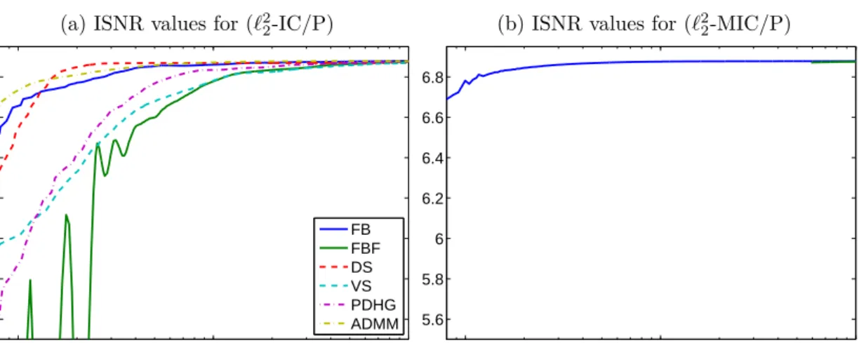

![Figure 4.5: The evolution of the values of the objective function and of the ISNR (im- (im-provement in signal-to-noise ratio) for Algorithm 3.293.29 (DR1), Algorithm 3.313.31 (DR2) and the forward-backward-forward method (FBF) from [58 58, Theorem 3.1].](https://thumb-us.123doks.com/thumbv2/123dok_us/8990780.2796959/121.892.156.758.124.341/evolution-objective-function-provement-algorithm-algorithm-backward-theorem.webp)


