An online learning algorithm for technical trading

Nicholas John Murphy

Supervisor: A/Prof. Tim Gebbie

A dissertation submitted in partial fulfilment of the requirement

for the Master of Science degree in Advanced Analytics,

School of Statistical Sciences,

University of Cape Town.

July 13, 2019

Abstract

We use an adversarial expert based online learning algorithm to learn the optimal parameters required to maximise wealth trading zero-cost portfolio strategies. The learning algorithm is used to determine the relative population dynamics of technical trading strategies that can survive historical back-testing as well as form an overall aggregated portfolio trading strategy from the set of underlying trading strategies im-plemented on daily and intraday Johannesburg Stock Exchange data. The resulting population time-series are investigated using unsupervised learning for dimensionality reduction and visualisation. A key contribution is that the overall aggregated trading strategies are tested for statistical arbitrage using a novel hypothesis test proposed by

1

University

of

Cape

2

Jarrowet al. [31] on both daily sampled and intraday time-scales. The (low frequency) daily sampled strategies fail the arbitrage tests after costs, while the (high frequency) intraday sampled strategies are not falsified as statistical arbitrages after costs. The estimates of trading strategy success, cost of trading and slippage are considered along with an offline benchmark portfolio algorithm for performance comparison. In addi-tion, the algorithms generalisation error is analysed by recovering a probability of back-test overfitting estimate using a nonparametric procedure introduced by Bailey

et al. [19]. The work aims to explore and better understand the interplay between different technical trading strategies from a data-informed perspective.

Keywords: online learning, technical analysis, portfolio selection, back-testing, sta-tistical arbitrage, overfitting, Johannesburg Stock Exchange

The copyright of this thesis vests in the author. No

quotation from it or information derived from it is to be

published without full acknowledgement of the source.

The thesis is to be used for private study or

non-commercial research purposes only.

Published by the University of Cape Town (UCT) in terms

of the non-exclusive license granted to UCT by the author.

University

of

Cape

3

Acknowledgements

I would like to express my gratitude to my supervisor A/Prof. Tim Gebbie. His guid-ance, dedication, deep insight and knowledge of a wide variety of topics have been key attributes in assisting me in completing this journey. There was never a shortage of input and ideas from him, even when various unforeseen issues arose during the course of this research. I am really grateful to have had the opportunity to work with Tim over the past three years, during my honours and master’s studies.

I would also like to thank the Statistical Finance Research Group in the Depart-ment of Statistical Sciences for various useful discussions relating to the work. In particular, I would like to thank Etienne Pienaar, Lionel Yelibi and Duncan Saffy. I also thank Michael Gant for numerous valuable discussions with regards to the statis-tical arbitrage test.

Last but not least, I send my most heartfelt thanks to my parents and my sister, who have provided unconditional support and remained patient with me over the past couple of years. I also thank my friends - without them, this journey would not have been complete. It has been a great experience, with both highs and lows, but those close to me have kept me going with their constant moral support and encouragement so, I thank them for that.

Related Publications and Pre-prints

Much of the content contained in this paper has been submitted in the form of a pre-print to the arXiv.org e-Print archive and is titled “Learning the population dynamics of technical trading strategies” [70].

5

Declaration

I hereby declare that this dissertation submitted in partial fulfilment of the require-ment for the Master of Science degree in Advanced Analytics is my own work except where specific reference is made to the work of others. The contents of the dissertation have not been submitted in whole or in part for a prior qualification at this university or any other university.

Contents

1 Introduction 13

1.1 Overview of this Study . . . 17

2 Online Portfolio Selection 18 2.1 Online vs. Offline Algorithms . . . 18

2.2 The Portfolio Selection Problem . . . 19

2.3 Offline Benchmark Strategies . . . 20

2.3.1 Buy-and-Hold Strategy . . . 20

2.3.2 Best Stock Strategy . . . 20

2.3.3 Constant Rebalancing Strategy . . . 20

2.3.3.1 BCRP Benchmark Algorithm . . . 21

2.4 Universal Portfolio Algorithm . . . 21

2.5 Meta-Learning Algorithms . . . 22

3 Technical Analysis 22 3.1 Technical Indicators and Trading Rules . . . 23

3.1.1 Simple Moving Average . . . 23

3.1.1.1 SMA Indicator: SMAc_t(n) . . . 23

3.1.1.2 Moving Average Crossover Trading Rule . . . 23

3.1.2 Exponential Moving Average . . . 24

3.1.2.1 Exponential Moving Average Crossover Rule . . . 24

3.1.2.2 EMA Indicator: EMAc_t(n). . . 24

3.1.3 Highest High . . . 24

3.1.4 Lowest Low . . . 25

3.1.5 Ichimoku Kinko Hyo . . . 25

3.1.5.1 Ichimoku Kinko Hyo Indicators . . . 25

3.1.5.2 Ichimoku Kinko Hyo Strategies . . . 25

3.1.6 Momentum . . . 27

3.1.6.1 Momentum Indicator: MOMt(n) . . . 27

3.1.7 Momentum Trading Rule . . . 27

3.1.8 Acceleration . . . 27

3.1.8.1 Acceleration Indicator: ACCt(n) . . . 27

3.1.8.2 Acceleration Trading Rule . . . 27

3.1.9 Moving Average Convergence/Divergence Oscillator . . . 27

3.1.9.1 MACD Indicators: MACDt(n1, n2) . . . 28

3.1.9.2 MACD Trading Rule . . . 28

3.1.10 Fast Stochastics . . . 28

3.1.10.1 Fast Stochastic Indicators . . . 29

3.1.10.2 Fast Stochastic Trading Rule . . . 29

3.1.11 Slow Stochastics . . . 29

3.1.11.1 Slow Stochastic Indicators . . . 29

3.1.11.2 Slow Stochastic Trading Rule . . . 29

3.1.12 Relative Strength Index . . . 30

3.1.12.1 RSI Indicator: RSIt(n). . . 30

3.1.12.2 RSI Trading Rule . . . 30

3.1.13 Moving Average Relative Strength Index . . . 31

3.1.13.1 MARSI Indicator: MARSIt(n1, n2) . . . 31

3.1.13.2 MARSI Trading Rule . . . 31

CONTENTS

7

3.1.14.1 Bollinger Band Indicator: Bollm_t (n) . . . 32

3.1.14.2 Bollinger Trading Rule . . . 32

3.1.15 Price Rate-Of-Change . . . 32

3.1.15.1 PROC Indicator: PROCt(n) . . . 32

3.1.15.2 PROC Trading Rule . . . 32

3.1.16 Williams %R . . . 33

3.1.16.1 Williams %R Indicator: Willt(n) . . . 33

3.1.16.2 Williams %R Trading Rule . . . 33

3.1.17 Parabolic SAR . . . 33

3.1.17.1 SAR Indicator: SAR(n) . . . 33

3.1.17.2 SAR Trading Rule . . . 34

3.2 Trend Following and Contrarian Mean Reversion Strategies . . . 34

3.2.1 Zero-Cost BCRP . . . 34

3.2.2 Zero-Cost Anti-BCRP . . . 34

3.2.3 Zero-Cost Anti-Correlation . . . 35

4 Data and Data Processing 35 4.1 Daily Data . . . 35

4.2 Intraday-Daily Data . . . 36

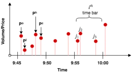
4.2.1 Time Bar Aggregation . . . 36

5 Learning Technical Trading 37 5.1 Expert Generating Algorithm . . . 38

5.1.1 Technical Trading . . . 38

5.1.2 Transforming Signals into Weights . . . 39

5.2 Online Learning Algorithm . . . 41

5.3 Algorithm Implementation for Intraday-Daily Trading . . . 46

5.4 Trading in Volume-time . . . 50

5.5 Transaction Costs and Market Frictions . . . 50

5.5.1 Volatility Estimation for Transaction Costs . . . 52

5.5.1.1 Daily Data Estimation . . . 52

5.5.1.2 Intraday Data Estimation . . . 52

6 Testing for Statistical Arbitrage 53 6.1 Outline of the Statistical Arbitrage Test Procedure . . . 56

7 Probability of Back-test Overfitting 57 7.1 Back-test Overfitting Framework . . . 58

7.2 CSCV Procedure . . . 59

8 Results and Analysis 61 8.1 Daily Data . . . 61 8.1.1 No Transaction Costs . . . 61 8.1.2 Transaction Costs . . . 69 8.2 Intraday-Daily Data . . . 70 8.2.1 No Transaction Costs . . . 72 8.2.2 Transaction Costs . . . 77 9 Conclusion 78 9.1 Future Work . . . 81 10 References 82

11 Appendices 86

A Data Related Appendices . . . 86

A.1 JSE TOP 40 Sector Constituents: Daily Data . . . 86

A.2 JSE TOP 40 Sector Constituents: Intraday Data . . . 86

B Work flow for Learning Class . . . 87

List of Figures

2 Example of the Ichimoku Kijun Sen Cross strategy implemented on 9 months of AGL data . . . 26

3 Example of the MACD trading rule implemented on 9 months of AGL data . . . 28

4 Example of the RSI trading rule implemented on 9 months of AGL data 31 5 Illustration of how trades arriving at irregular time intervals are sam-pled over regular intervals (5-minutes). . . 37

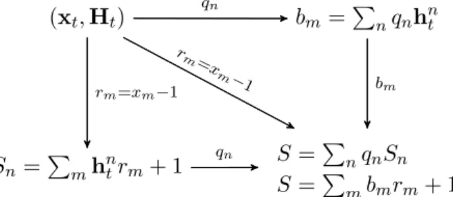
6 Relationship between the components of the Online Learning Algorithm 46 7 Figure7(a)illustrates the overall cumulative portfolio wealth (S) of the online learning algorithm (OLA - blue) against the benchmark BCRP strategy (orange) and Figure7(b)illustrates the associated profits and losses (PL) for daily trading without transaction costs. . . 62

8 Figure8(a)illustrates the expert wealth (Sh) for all Ω experts for daily data with no transaction costs. Figure8(b)illustrates the mean expert wealth of all experts for each trading strategy (ω) for daily data with no transaction costs. . . 63

9 Figure 9(a) and Figure 9(b) show the latent space of a Variational Autoencoder on the time series of expert wealth’s, implemented using Keras in Python. In Figure9(a)experts are coloured by which of the 4 object clusters they trade whereas in Figure9(b), experts are coloured by their underlying trading strategyω(i). . . 66

10 Histogram of the 5000 simulated Min-t statistics resulting from the CM test implemented on the simulated incremental process given in Eq. (58) along with the Min-tstatistic (green) for the overall strategy’s profit and loss sequence over the 400-day period stretching from the 30th _{trading day until the 430}th _{trading day without any account for} transactions costs. . . 67

11 Probability of the overall trading strategy generating a loss after for each of the 30 days from the first trading day through until the 30th trading day. . . 68

12 Probability of back-test overfitting for 30 simulations of the online learn-ing algorithm on daily historic data. . . 69

13 Profits and losses (PL) for overall strategy for daily trading with trans-action costs. . . 70

LIST OF FIGURES

9

14 Figure 14(a) illustrates the histogram of the 5000 simulated Min-t statistics resulting from the CM model and the incremental process given in Eq. (58) along with the Min-t statistic (green) for the overall strategy’s daily trading profit and loss sequence over the 400-day period stretching from the 30th _{trading day until the 430}th _{trading day with} transactions costs incorporated. Also illustrated is the critical value at the 5% significance level (red). Figure 14(b) shows the probability of the overall trading strategy generating a loss for each of the first 400 trading days. . . 71 15 Fig.15(a)shows the overall cumulative portfolio wealth (S) for

intraday-daily trading with no transaction costs. Fig.15(b)illustrates the profits and losses (PL) for overall strategy for intraday-daily trading with no transaction costs. . . 73 16 Fig.16(a)illustrates the expert wealth (Sh) for all Ω experts for

intraday-daily trading with no transaction costs. Fig.16(b)illustrates the mean expert wealth of all experts for each trading strategy (ω(i)) for intraday-daily trading with no transaction costs. . . 74 17 Histogram of the 5000 simulated Min-t statistics resulting from the

profit and loss process without transaction costs taken into account along with the Min-t statistic for the overall strategy (green) and the critical value at the 5% significance level (red). The profit and loss process is extracted from the 6th _{time bar on the second day, which} corresponds to the period when active trading begins, until the 400th time bar hence. This corresponds to roughly four and a half days worth of trading profits. . . 75 18 Probability of the overall trading strategy generating a loss after n

periods for each n = 1, . . . ,30 of the intraday-daily profit and loss process (PL) without transaction costs. The profits and losses are taken starting from the 5th _{time bar of the second day when active} trading commences as the first day is required as a look-back for the daily trading component. . . 76 19 Probability of back-test overfitting for 20 simulations of the online

learn-ing algorithm on intraday-daily historic data. . . 77 20 Figure20(a)and Figure20(b)illustrate the overall cumulative portfolio

wealth (S) and profits and losses (PL) respectively for intraday-daily trading with transaction costs. . . 79 21 Figure 21(a) shows the histogram of the 5000 simulated Min-t

statis-tics resulting from the CM model and the incremental process given in Eq. (58). Also illustrated is the Min-t statistic (green) for the first 400 trading periods from commencement of active trading (5th_{time bar of} the second day) for intraday-daily profit and losses with transaction costs incorporated along with the critical value at the 5% significance level (red). Figure 21(b)illustrates the probability of the overall trad-ing strategy generattrad-ing a loss afternperiods for eachn= 1, . . . ,30 of the intraday-daily profit and loss process (PL) with transaction costs incorporated commencing from the first period of active trading (5th time bar of the second day). . . 80 22 State flow diagram for the MATLAB learning class . . . 87

List of Tables

1 Variable definitions . . . 12

2 Ichimoku Kijun Sen Cross strategy . . . 25

3 Momentum trading rule . . . 27

4 Acceleration trading rule . . . 27

5 MACD trading rule . . . 28

6 Fast stochastic trading rule . . . 29

7 Slow stochastic trading rule . . . 30

8 Relative strength index (RSI) trading rule . . . 30

9 MARSI trading rule . . . 31

10 Bollinger trading rule . . . 32

11 Price rate of change (PROC) trading rule . . . 32

12 Williams %R trading rule . . . 33

13 SAR trading rule . . . 34

14 Algorithm for the expert generating function. . . 42

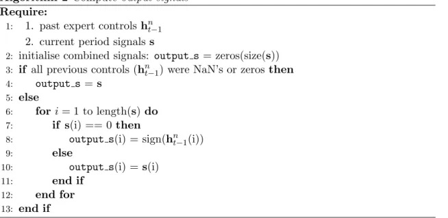
15 Algorithm for the controls function which transforms trading signals into portfolio controls. In the above algorithm, output s refers to output signals (combined signals) as discussed in Section5.1.2. . . 43

16 Algorithm which transforms output signals into portfolio controls using the volatility loading method. The algorithm follows from Algorithm2 and is part of the control function called by Algorithm 1. Note that output s≤0 (or≥) implies thatoutput s(i)≤0 (or≥) for eachi. . 44

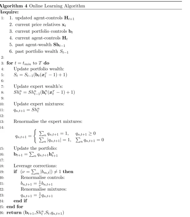
17 Algorithm for Online Learning. . . 47

18 Group summary statistics of the overall rankings of experts grouped by their underlying strategy (ω(i) where i = 1, . . . ,17) for the daily trading. In brackets next to mean are the mean overall ranking of experts utilising each strategy. . . 64

19 Group summary statistics of the expert’s profits and losses per period grouped by their underlying strategy (ω(i) wherei= 1, . . . ,17). . . 65

20 Group summary statistics of the overall rankings of experts grouped by their underlying strategy (ω(i) wherei= 1, . . . ,17) for intraday-daily trading. In brackets are the mean overall ranking of experts utilising each strategy. . . 72

List of Variables

Variable Definition

ω parameter of underlying strategy of a given expert which corre-sponds to one of the technical trading strategies or trend-following strategies. ω(i) is then theith_{strategy from the set of all} strate-gies

W1 number of trading strategies which utilise one parameter W2 number of trading strategies utilising two parameters W total number of trading strategies: W =|ω|=W1+W2

n1 vector of short-term look-back parameters

n2 vector of long-term look-back parameters L number of short-term look-back parameters

LIST OF TABLES

11

K number of short-term look-back parameters

c object clusters parameter wherec(i) is theithobject cluster C number of object clusters

Ω total number of experts (this is different to the bold omegaΩused in the probability of back-test overfitting framework)

ADV average daily volume

δliq number of periods to look-back to compute the ADV and choose themmost liquid stocks

m number of stocks to be passed into the expert generating algorithm ranked by their liquidity

hn_t nthexpert’s strategy (m+ 1 portfolio controls) for period t Ht expert control matrix by made up of all n experts’ strategies at

timetfor allmstocksi.e. Ht= [h1t, . . . ,h n t] Sht wealth of allnexperts at timet

Shn

t nthexpert’s wealth at timet

bt final overall aggregate portfolio to be used in the following period t+ 1 which we denote

S vector of the overall aggregate portfolio compounded wealth over time

St overall aggregate portfolio compounded wealth at timet

PL vector of the overall aggregate portfolio cumulative profits and losses

PLt the overall aggregate portfolio cumulative profits and losses at timet

nb(ns) number of buy (sell) signals from the set of output signals

σ+ (σ−) vector of standard deviations of stocks to be bought (sold)

w m+ 1 vector of weights allocated to m stocks and the risk-free asset

wrf weight allocated to the risk-free asset

tmin time period at which trading commences (either daily/intraday) T terminal time of trading (generally daily but can be either

dai-ly/intraday)

Xt m×5 matrix of stock’s OHLCV values at each time period t (either daily/intraday)

Xd daily OHLCV data

XI intraday OHLCV data

xt vector ofm+ 1 price relatives at time periodt

Pc_t vector of closing prices for allmstocks at time periodt Pc

m,t closing price of stockmat time periodt tI tthI time bar of a given day

TI final (terminal) time bar of a given day (4:30pm) HF_t,T

I fused intraday-daily expert control matrix hFn,t,TI n

th_{expert’s controls for allmassets at time bart}

I on thetthday ShF_t,tI fused intraday-daily expert wealth vector for allnexperts for the

tth_I time bar on thetthday ShF

n,t,TI+1 n

th_{expert’s wealth at time bart}

I on thetthday σ volatility of the returns of a stock

ν(t) cumulative discounted trading profits/losses at timet

∆νt cumulative discounted trading profit/loss increment at timeti.e. ∆νt=ν(t)−ν(t−1)−1

Min-t statistic used to make inferences regarding the no statistical arbi-trage null hypothesis

TBL back-test length for each of theN separate trial simulations of the algorithm

N number of back-test trials performed on independent subsets of historic data (N=bT /TBLctrial simulations)

N! number of permutations of the set (1, . . . , N) which ranks theN back-test trials

R(R) IS (OOS) performance of theN back-tests for a fixed performance measure (Sharpe Ratio)

RC(RC) performances for a pair of IS (OOS) sample subsets ofR(R) Ω ranking space ofN! (This bold and capitalized omega is different

from the one used to denote the total number of experts as referred to previously in the study which is not bold (Ω))

r(r) rankings of trials in the vectorR(R) withnth_elementr n (rn) Ω∗_n subspace of vectors of back-test trials’ performance rankings f

({f ∈ Ω|fn = N} of Ω where f = (f1, . . . , fn)), such that the nth_{back-test trial has the highest rankingi.e. f}

n=N

1. INTRODUCTION

13

1

Introduction

Selecting plausible trading strategies, and allocating wealth among these strategies, in order to maximise wealth over multiple decision periods can be a difficult task. An approach to combining strategy selection with wealth maximisation is to use online or sequential machine learning algorithms [1]. Online portfolio selection algorithms attempt to automate a sequence of trading decisions among a set of stocks with the goal of maximizing return in the long run.1 _{Such algorithms typically use historical} market data to determine, at the beginning of a trading period, a way to distribute their current wealth among a set of stocks. These types of algorithms can use many more features than merely price, so called “side-information” [2], but the principle remains that same. The attraction of this approach is that the investor does not need to have any knowledge about the underlying distributions that could be generating the stock prices (or even if they exist). The investor is left to “learn” the optimal portfolio to achieve maximum wealth using past data directly [1].

Cover [3] introduced a “follow-the-winner” online investment algorithm2_{called the} Universal Portfolio (UP) algorithm3_{. The basic idea of the UP algorithm is to allocate} capital to a set of experts characterised by different portfolios or trading strategies; and to then let them run while at each iterative step to shift capital from losers to winners to find a final aggregate wealth.

Here our “experts” will be similarly characterised by a portfolio (or trading strat-egy) where a particular agent makes decisions independently of all other experts. The UP algorithm holds parametrized constant rebalanced portfolio (CRP) strategies as it’s underlying experts. We will have a more generalised approach to generating ex-perts. The algorithm provides a method to effectively distribute wealth among all the CRP experts such that the average log-performance of the strategy approaches the best constant rebalancing portfolio (BCRP) which is the hindsight strategy chosen which gives the maximum return of all such strategies in the long run. The key inno-vation that Cover [3] provided was a mathematical proof for this claim based on an arbitrary sequences of ergodic and stationary stock return vectors.

It is important to realise that if there exists some log-optimal portfolio such that no other investment strategy has a greater asymptotic average growth then to achieve this one must have full knowledge of the underlying distribution and of the generating process to achieve such optimality [2,3,4,5]. Such knowledge is unlikely in the context of financial markets. However, strategies which achieve an average growth rate which asymptotically approximates that of the log-optimal strategy is possible given that the underlying asset return process is sufficiently close to being stationary and ergodic. Such a strategy is calleduniversally consistent. Gyorfiet al. [5] proposed a universally consistent portfolio strategy and provided empirical evidence of a strategy based on nearest-neighbour based experts which reflects such asymptotic log-optimality.

The idea is to match current price dynamics with similar historical dynamics (pat-tern matching) using a nearest-neighbour search algorithm to select parameters for 1

Here, the long run will depend on the frequency at which trading occurs. This could imply anything from a few days to a few weeks for high frequency trading algorithms and a few months (years) for daily (weekly) trading algorithms

2_{follow-the-winneralgorithms give greater weightings to better performing experts or stocks} 3

experts. The algorithm was extended by Loonat and Gebbie [6] in order to implement a zero-cost (long/short and self-financing) portfolio selection algorithm via a quadratic approximation derived from the mutual fund separation theorems to allow the algo-rithm to be more effectively considered in the context statistical arbitrage trading. The algorithm was also re-cast to replicate near-real-time applications using look-up libraries learnt offline. However, there is a computational cost associated with cou-pling creation of offline pattern libraries - the algorithms are not truly online4_{. A key} objective in the implementation online learning in this work is that the underlying experts here are online too; they can be sequentially computed on a moving finite data-window using parameters from the previous time step - rather than having the need to search data-histories or make comparisons with a library of patterns learnt offline.

Here we ignore the pattern matching step in the aforementioned algorithm and rather propose our own expert generating algorithm using tools from technical anal-ysis. Concretely, we replace the pattern-matching expert generating algorithm with a selection of technical trading strategies. Technical trading refers to the practice of using trading strategies (rules) derived technical analysis indicators which use mathe-matical formulas based on prices, volume traded or a combination of both to generate trading signals [7,8]. They claim to be able to exploit statistically measurable short-term market opportunities in stock prices and volume by studying recurring patterns in historical market data [9,10,11]. An abundance of indicators has been developed over the years with some proving to be more successful than others. Indicators per-form differently under different market conditions which is why traders will often use multiple indicators to confirm the signal that one indicator gives on a stock with an-other indicator’s signal. Thus, in practice and various studies in the literature, many trading rules generated from indicators are typically back tested on a sufficient amount of historical data to find the rules that perform the best. This is typically known as data mining. One must be careful when using data mining to test the performance of many rules since the chance of a “lucky”5 performance of a given rule from the set will increase leading to biased results [12]. This is often what motivates the need to implement rigorous statistical analysis and back-tests to determine which rules per-form consistently well.

Traditionally, technical analysis has been a visual activity, whereby traders study the patterns and trends in charts, based on price or volume data, and use these di-agnostic tools in conjunction with a variety of qualitative market features and news flow to make trading decisions. Many studies have criticised the lack of a solid mathe-matical foundation for many of the proposed technical analysis indicators [12,13,14]. There has also been an abundance of academic literature, utilising technical analysis for the purpose of trading and several studies have attempted to develop indicators and test them in a more mathematically, statistically and numerically sound manner [12,15,16]. However, much of this work needs to be viewed with some suspicion - it is extremely unlikely that this or that particular strategy or approach was not the result of some sort of back-test overfitting [17,18,19]. Many studies attempt to predict the future movements of prices using technical analysis with mixed success [9,11,20,21]. This work does not address the question: Which, if any, technical analysis based 4

See Section2.1for an explanation on online vs offline algorithms

5_{Luck, in the sense that it may lead to a favourable but accidental correspondence between trends in}

1. INTRODUCTION

15

methods reveal useful information for trading purposes? Rather we aim to bag a collection of technical experts and allow them to compete in an adversarial manner, using the online learning algorithm, to then consider whether the resulting aggregate strategy passes a reasonable test for statistical arbitrage, and has a relatively low probability of being the result of back-test overfittingi.e. it could generalise well out-of-sample.

Here we will be concerned with the idea of understanding whether the collec-tive population of technical experts can through time lead to dynamics that can be considered a statistical arbitrage [22] with a reasonably low probability of back-test over-fitting [19]. More specifically, can we generate wealth (before costs) using the online aggregation of technical strategies? Then, what broad groups of strategies will emerge as being successful (here in the sense of positive trading profits with declining variance in losses)? When measuring success, of utmost importance is the consider-ation of the transaction costs inherent in trading. One of the earliest studies which looked at profitability of filter rules6revealed that such trading rules were unprofitable after transaction costs were taken into account [32]. Any reasonable book on trad-ing/investing will certainly contain a section on transaction costs, and if not, will at least have short discussions on the impact of costs on back-test performance of such algorithms [7,12,15,33,34]. Costs are always a plausible explanation for any appar-ently profitable trading strategy (see [6]), and after costs, there exists a high-likelihood that there was a healthy amount of data over-fitting; given that we only have single price paths from history, and have little or no knowledge about the probability of the particular path that has been measured.

Another important consideration for traders is whether a market is efficient, and hence, whether they can consistently profit from trading in the market. Here efficiency refers to the expeditiousness of market prices to incorporate new information at any time. Thus, in an efficient market, all known and relevant information is presumed to be reflected in prices almost instantaneously [12]. This is the idea behind the popular hypothesis that has been researched and debated for many years, and is known as the Efficient Market Hypothesis (EMH), developed in the groundbreaking work of Fama [23]. Historically, financial theory supported the view that markets are in fact efficient resulting in market price moments that follow a random walk or Brownian motion. This implies that past price movements cannot be used to predict future movements and hence, an efficient market is trend-less and unpredictable. In line with this idea is the statement that “an average investor- whether an individual, pension fund, or a mutual fund- cannot hope to consistently beat the market, and the vast resources that such investors dedicate to analysing, picking and trading securities are wasted” [24]. This isn’t to say that an investment (trading) strategy, such as those generated from technical indicators, cannot generate a positive return, but when the strategy is risk-adjusted, then it will not consistently provide better returns than the market benchmark [12]. In order to beat the market benchmark consistently, an investor will have to take on much higher levels of risk, possibly leading to significant losses. Today, it is generally accepted that markets are in fact inefficient.

A similar train of thought to that of the EMH was introduced by Lo [25], which argues that the efficiency of markets is determined by the dynamics of evolution, and 6

Filter rules are a technical trading rule whereby a trader is signalled to take action by buying or selling a stock when it’s price rises or falls by a certain percentage (often in relation to a previous high or low)

introduces a new paradigm called the Adaptive Market Hypothesis (AMH). The AMH had a similar direction to the original approaches suggested by Farmer and Lo [26] and Farmer [27] in applying evolutionary principles to financial markets. Farmer and Lo [28] describe the universe of computer algorithms as a complex ecology of highly specialized, highly diverse, and strongly interacting agents. This in turn leads to the co-evolution of human trading, computer trading, markets and regulators. They argue that the role computers play in markets can only be understood from an ecological and evolutionary perspective, in a sense that these computers are designed by considering historical incidences in markets, but also specific details such as the design of markets, regulations and patterns in trading. As markets conditions constantly change, new computer systems and trading strategies need to be designed as previous systems and strategies often become unprofitable and/or unsuccessful. This is why the adoption of machine learning in automated trading systems has recently exploded, as such sys-tems are often able to adapt and learn which strategies are becoming more (or less) profitable and hence allocate greater (or smaller) capital amounts for such strategies. This has led to the belief that, with less human involvement in active decision making in trading and investing, that markets are bound to become more efficient, however this is highly debatable.

Rather than considering various debates relating the technicalities of market effi-ciency, we restrict ourselves to market efficiency in the sense used by Fischer Black [29, 30]. This is the situation where some of the short-term information is in fact noise, and that this type of noise is a fundamental property of real markets. Although market efficiency may plausibly hold over the longer term, in the short-term there may be departures that are amenable to tests for statistical arbitrage [31], departures that create incentives to trade, and more importantly departures that may not be easily traded out of the market due to various asymmetries in costs and market access. The proposed trading strategies in this work are tested in this sense.

In order to analyse whether the overall back-tested strategy depicts a candidate statistical arbitrage, we implement a test first proposed by Hoganet al. [22] and then further refined by Jarrowet al. [31]. Hoganet al. provide a plausible technical defi-nition of statistical arbitrage based on a vanishing probability of loss and variance in the trading profits, and then use this to propose a test for statistical arbitrage using a Bonferroni test [22]. This methodology was further extended and generalized by Jar-rowet al. to account for the asymmetry between desirable positive deviations (profits) and undesirable negative deviations (losses), by including a semi-variance hypothesis instead of the originally constructed variance hypothesis, which does not condition on negative incremental deviations [31]. The so-called Min-t statistic is computed and used in conjunction with a Monte Carlo procedure to make inferences regarding a carefully defined “no statistical arbitrage” null hypothesis.

This is analogous to evaluating market efficiency in the sense of the Noisy efficient market hypothesis [29] whereby a failure to reject the no statistical arbitrage null hy-pothesis will result in concluding that the market is in fact sufficiently efficient and no persistent anomalies can be consistently exploited by trading strategies over the long term. Traders will always be inclined to employ strategies which depict a statistical arbitrage and especially strategies which have a probability of loss that declines to zero quickly as such traders will often have limited capital and short horizons over which they must provide satisfactory returns (profits) [31].

1. INTRODUCTION

17

1.1

Overview of this Study

We make the effort here to be very clear that we do not attempt to identify profitable (technical) trading strategies, but rather we will generate a large population of strate-gies (experts) constructed from various technical trading rules and combinations of the associated parameters of these rules in the attempt to learn the aggregate pop-ulation dynamics of the set of experts. Expert’s will generate trading signals (buy, sell or hold) for each stock held in their portfolio based on the underlying parameters and the necessary historic data implied by the parameters. Once trading signals for the current time period t have been generated by a given expert, a methodology to transform the signals into a set of portfolio weights (controls) is required.

We introduce a transformation method that computes controls proportional to the relative volatilities of the stocks for which non-zero trading signals were gener-ated, and then normalise the resulting values such that the self-financing and leverage constraints required by the algorithm are satisfied. The resulting controls are then utilised to compute the corresponding expert wealth’s. The experts who accumulate the greatest wealth during a trading period, will receive more wealth in the follow-ing tradfollow-ing period, and thus contribute more to the final aggregated portfolio. This can be best thought of as some sort of “fund-of-funds” over the underlying collection of trading strategies. This is a meta-expert7 _{that aggregates experts that represent} all the individual technical trading rules. The overall meta-expert strategy perfor-mance is achieved by the online learning algorithm. Equity curves for the individual expert’s portfolios (the accumulated trading profit through time) along with perfor-mance curves for the overall strategy’s wealth and the associated profits and losses are provided.

We perform a back-test of the algorithm on two different data sets over two sep-arate time periods; one using daily data over a six-year period from 1 January 2010 to 29 April 2016 and the other using a mixture of intraday and daily data over a two and a half month period from 2 January 2018 to 21 March 2018. A selection of the fifteen most liquid stocks which constitute the Johannesburg Stock Exchange (JSE) Top 40 shares is utilised for the two separate implementations.8

The overall strategy performance is compared to the BCRP strategy to form a benchmark comparison to evaluate the success of our strategy. The overall strategy is then tested for statistical arbitrage to find that in both a daily and intraday-daily data implementation, the strategy depicts a statistical arbitrage. It must be cautioned that this is prior to accounting for costs which can be expected to shift the bias. The key point here (as in [6]) is that it does seem that plausible statistical arbitrages are detected on the meso-scale and in the short-term, however, for reasonable costing, it may well be that these statistical arbitrages exist because they cannot be profitable traded out of the system.

In addition, transaction cost analysis, the overall strategy’s probability of loss is computed to get an idea of the convergence of such losses to zero; most traders will be concerned about short-run losses. Finally, we analyse the generalisation error of the overall strategy to get a sense of whether or not the strategy conveys back-test overfitting by estimating the probability of back test overfitting inherent in multiple

7_{See Section2.5for a discussion on meta-learning algorithms} 8

simulations of the algorithm on subsets of historic data.

Throughout the study, we use the terms investing and trading interchangeably, however, we should distinguish the differences between the two. Investors buy stocks with the intention of gaining wealth over the long term by holding a stock which they believe will grow over the period. Investors typically use fundamental analysis9 _to identify long-term potential in a company (stock). Traders buy and sell stocks with the intention of making quick short-term profits on price differences of stocks.

The rest of the paper will proceed as follows: Section2 discusses the differences between online and offline algorithms and introduces online portfolio selection prob-lems, terminology, and various portfolio selection benchmark algorithms. Section 3 describes technical analysis and provides in-depth descriptions of all trading rules im-plemented in the project. Section4describes the data utilised in the study. Section5 explains the construction of the algorithm including details of how the experts are gen-erated, how their corresponding trading signals are transformed into portfolio controls and a step-by-step break-down of the learning algorithm. In Section6, we introduce the concept of a statistical arbitrage, including the methodology for implementing a statistical arbitrage test and the probability of loss for a trading strategy. All experi-ment results of impleexperi-mentations of the algorithm and extensive analysis is presented in Section 8. Section9 states all final conclusions from the experiments and possible future work.

2

Online Portfolio Selection

With regards to a multi-period online portfolio selection (OPS) algorithm, which is what our trading algorithm is based on, the goal is to sequentially rebalance the portfolios of each expert by allocating capital among the set of assets held by each expert with the goal of maximizing the investor’s terminal wealth irrespective of risk [2,3,6,36,37]. Here, the investor basically represents a weighted average portfolio of all the experts where each expert has its own strategy with which it uses to allocate it’s capital among the set of assets. The goal is to find the optimal portfolio by weighting each expert’s portfolio based on their performance. In achieving the growth optimal portfolio, no underlying statistical assumptions are made as the portfolio wealth is solely dependent on the data [2,3]. The details of OPS algorithms will be discussed in more depth in the following subsections.

2.1

Online vs. Offline Algorithms

Traditionally, the design and analysis (back-tests) of many trading algorithms has been conducted on static data sets where the algorithm is executed on an entire batch of data as an input to the algorithm. However, in practice, often the input data is only partially available since some relevant input data arrives in a sequential manner as time moves forward and markets and traders react to evolving market data and conditions [35]. The process whereby the algorithm learns and updates parameters sequentially as data arrives is also known as online learning which is in contrast to

9

Fundamental analysis attempts to measure the intrinsic value of a stock by using economic factors (fundamentals) of the company included in financial statements such as Earnings Per Share, Return On Equity, Revenue and price to earnings ratio to name a few [42,11]

2. ONLINE PORTFOLIO SELECTION

19

offline (batch) learning, whereby the algorithm updates parameters given that an en-tire batch of static data is available. Contrary to offline learning, where a decision is completely irrelevant to previous decisions, during online learning one decision is dependent to prior decisions made by the algorithm [36]. Online learning becomes more significant when trading is executed at higher frequencies as the algorithm needs to react faster to market events being streamed into the algorithm at high speeds and be computationally efficient enough to make decisions at high rates.

2.2

The Portfolio Selection Problem

The basic portfolio selection problem involves an investor who invests his capital in a market with m stocks over T trading periods. Suppose that at the tth period (t= 1, . . . , T), the stocks have closing prices Pc_t = (p1, . . . , pm) where pi is the price of theith_{stock at time periodt. Let the price changes of the stocks be represented by} price relatives10_{which are just ratios of the prices of each stockiat timetto the prices} at timet−1, that is,xi,t=

pi,t

pi,t−1 where the price relatives for thet

th_{period are given} byxt= (x1,t, . . . , xm,t) and the sequence of relatives over the entire investment period are given by X = (x1, . . . , xT). Resultantly, an investment in stock i over period t will increase by a factor ofxi,t [36]. Denote aportfolio bybt= (b1,t, . . . , bm,t), where bi,t represents the amount of wealth allocated to stockiat the beginning of periodt. Theportfolio strategy over theT periods is thus the sequence of portfolios

B=b1, . . . ,bT (1)

where b1 = (1/m, . . . ,1/m). Then, at time t, the wealth of the investment in-creases by a factor of St= m X i=1 bi,txi,t (2) =b|_t ·xt (3)

Suppose we initially invest an amountS0and reinvest the wealth after each period subsequent to accounting for profits and losses. In such a case, the portfolio’s wealth grows multiplicatively over time [36]. Thus, the total cumulative wealth at the end of T periods adopting a portfolio strategyBwith realised price relativesXwill be

ST(B,X) =S0 T

Y

t=1

b|t ·xt (4)

For future reference to Eq. (4), we will drop the argument for the price relative sequenceXso thatST(B) =ST(B,X). The aim is for the investor is to sequentially update (rebalance) the portfolio (bt) at each timetas he realises the price relative for the previous period (xt−1) in order to achieve some target. The portfolio is rebalanced

by buying and selling the stocks based on whether their prices have dropped or risen respectively. Once thetthtrading period is complete, the price relativextis realised. Eq. (4) only holds in the long-only portfolio case, however for our purposes, we have

10

Price relatives (simple gross return) are used in most literature on portfolio selection problems but we could replace these with a simple net return given byxi,t=

pi,t−pi,t−1 pi,t−1 [36].

to account for the possibility that a short position is taken in a stock. The adjusted equation for the cumulative wealth of a long/short portfolio is as follows [6]

ST(B,X) =S0 T

Y

t=1

[b|_t ·(xt−1) + 1] (5)

2.3

Offline Benchmark Strategies

Before discussing the various OPS algorithms from the literature which form the basis of our algorithm, we need to introduce some of the benchmark principles for OPS which we can use to measure the performance of our algorithms against. We will discuss the three most common benchmark strategies and all three of these are offline11 benchmarks.

2.3.1

Buy-and-Hold Strategy

The first benchmark is thebuy-and-hold (BH) portfolio strategy is the simplest and one of the most popular benchmarks. Here, an investor will buy an initial portfolio of stocks,b1, at the beginning of the 1stperiod and hold it until the end of the investment horizon without adjusting it [37, 39]. A specific type of BH strategy is the uniform buy-and-hold (UBH) strategy and corresponds to the case whereb1= (1/m, . . . ,1/m)

i.e. an equal holding of each stock in the portfolio.

2.3.2

Best Stock Strategy

The best stock strategy is just a special case of the BH strategy and is simply the optimal in hindsight BH strategy [38] whereby the investor will invest all his wealth in the best stock (in hindsight).

2.3.3

Constant Rebalancing Strategy

Theconstant rebalancing portfolio (CRP) is a portfolio strategy which rebalances the portfolio to have a fixed proportion in every stock at the beginning of each trading period t (bt = bt+1) [39]. Borodin et al. [38] show that the optimal in hindsight CRP known as the best constant rebalancing portfolio (BCRP) will always performs at least as well as the best stock strategy and can often significantly outperform the best stock by taking advantage of market fluctuations. Furthermore, Cover [3] shows that this portfolio has the greatest exponential growth in hindsight among all possible BH portfolio allocations. CRP strategies form the basis for much of the theory from which our algorithm is developed from. Given that b= B = b1 = · · · =bT and following from Eq. (4), the cumulative wealth of a long-only CRP strategy with targeted portfoliobis ST(b) =S0 T Y t=1 b|·xt (6)

and the corresponding cumulative wealth where short selling is permitted

ST(b) =S0 T Y t=1 [b|·(xt−1) + 1] (7) 11

2. ONLINE PORTFOLIO SELECTION

21

2.3.3.1

BCRP Benchmark Algorithm

To get an idea of how well our online algorithm performs, we compare its performance to that of the offline BCRP. There are two possible methods to finding the controls for the BCRP strategy: 1) an analytical method that requires the use of Kuhn-Tucker methods to solve a Lagrangian function involving the expected utility of wealth with respect to a constant relative risk aversion [40] 2) brute force Monte Carlo method [41]. To find the portfolio controls of such a strategy, we perform a brute force Monte Carlo approach to generate 5000 random CRP strategies on the entire history of price relatives and choose the BCRP strategy to be the one that returns the maximal terminal portfolio wealth. As a note here, the CRP strategies we consider for the Monte Carlo simulation are long-only portfolios. Section8illustrates the performance of this method against that of our proposed learning method which will be introduced and discussed in detail in Section5.

2.4

Universal Portfolio Algorithm

One of the most popular OPS algorithms is the Universal Portfolio (UP) algorithm introduced by Cover [3]. Cover introduces a concept known as universality in order to classify a specific type of OPS algorithm. The basic idea of these algorithms is to track the BCRP of any arbitrary sequence of price relatives (returns).

The algorithm was later refined by Cover and Ordentlich [2] and was called the µ-Weighted Universal Portfolio. Here, µ is a given distribution on the simplex Bm which represents the space of all valid portfolio strategies of dimension m. Validity requires thatBm={b∈Rm|bi≥0 and P

m

i=1bi = 1}. Consider Ω12 experts whereby each expert ω invests in m stocks utilising their own CRP strategy. Thus, each expert will have his own unique fixed portfolio allocation, say bω ∈ Bm. Suppose that a proportion of wealthdµ(bω) is invested into each expert. Then, following from Eq. (6), thet-period wealth of theωth_{expert be given byS}

t(bω)dµ(bω) where St(bω) = T Y t=1 b|·xt (8) andS0(bω) = 1.

In the case that the simplex in continuous, the update rule for the universal port-folio at the beginning of the (t+ 1)th_{time period is given by [2]}

bU Pt+1= R BmbSt(b)dµ(b) R BmSt(b)dµ(b) (9)

where the rule is initialised with b1 = (_m1, . . . ,_m1). However, if the simplex is discrete (which is what we assume in this study13_{), the universal portfolio for Ω} experts is given by bU P_t+1= PΩ ω=1b ω St(bω) PΩ ω=1St(b ω₎ (10) 12

ωcan either be finite or infinite. IfBmis a continuous simplex then there are infinite experts (ω=∞) and if the simplex is discrete then there are a finite number of experts

13

Eq. (10) will form the basis of the updating rule for our learning algorithm (see Section 5.2). We can show that the terminal wealth of the UP algorithmST(bU P) is in fact the average of all the experts wealth’s [37]

ST(bU P) = T Y t=1 x|_t·bU P_t = T Y t=1 m X i=1 xi,t·bU Pi,t = T Y t=1 m X i=1 xi,t· PΩ ω=1b ω iSt−1(bω) PΩ ω=1St−1(b ω ) (by Eq. (10)) = T Y t=1 PΩ ω=1 Pm i=1(xi,t·b ω i)St−1(bω) PΩ ω=1St−1(bω) = T Y t=1 PΩ ω=1St(bω) PΩ ω=1St−1(bω) sinceSt(bω) =St−1 m X i=1 bωi ·xi,t = PΩ ω=1 QT t=1St(bω) PΩ ω=1 QT t=1St−1(bω) = PΩ ω=1ST(bω) PΩ ω=1S0(bω) = 1 Ω Ω X ω=1 ST(bω) since Ω X ω=1 S0(bω) = Ω X ω=1 1 = Ω

Hence, the UP algorithm can be considered as a BH strategy of all Ω experts.

2.5

Meta-Learning Algorithms

Meta-learning algorithms are very similar to the Universal Portfolio algorithm in that they are a ’follow-the-winner’ algorithm and take a performance weighted average of a set of underlying strategies however instead of using CRP-experts as in the Universal Portfolio algorithm, these algorithms handle a variety of different classes of experts [36]. Our proposed trading algorithm will mimic a meta-learning algorithm since each expert’s trading strategy will form a different class within the algorithm. Majority of the experts used in our algorithm will be developed from technical analysis and are discussed comprehensively in the following section.

3

Technical Analysis

Technical Analysis was formed on principles from Dow Theory [42] and uses the his-tory of market action14_{to predict future movements [20]. Over the past 2 decades, the} use of technical analysis for the generation of trading rules has been vast in academic literature and results have varied.

Technicians believe that anything that can possibly affect the price is actually reflected in the price and hence claim that market action should reflect all shifts in 14

3. TECHNICAL ANALYSIS

23

supply and demand [42] leading to the belief that market action is the best source of information. This implies that the technician is indirectly studying fundamentals since the data will reflect the up and down movements for given stocks in the market, however, it is important to note that technicians are not at all concerned with the rea-sons for these movements. They will make trading decisions based solely on market action and leave it to the fundamental analysts to explain the reasons for historical movements using news and other data.

We utilise fourteen trading rules built from technical analysis. There are typically three types of trade entry techniques: trend-following, oscillators and patterns [15]. The set of rules we consider contain a mixture of such techniques. A further three online portfolio selection techniques are implemented and are discussed in Section3.2.

3.1

Technical Indicators and Trading Rules

We follow Creamer and Freund [9] and Kestner [15] in introducing and describing some of the more popular technical analysis indicators as well as a few others that are widely available. We also describe in detail the trading rules associated with the technical indicators which generate buy, sell and hold signals, most of them described as in Creamer and Freund [9].

3.1.1

Simple Moving Average

The most common moving average is thesimple moving average (SMA). The SMA is the mean of a time series (typically of closing prices) over the lastntrading days and is usually updated every trading period to take into account more recent data and drop older values. The smaller the value of n, the closer the moving average will fit to the price data

3.1.1.1

SMA Indicator: SMA

(

n

)

SMAt(Pc, n) = 1 n n−1 X i=0 P_tc_−i (11)

3.1.1.2

Moving Average Crossover Trading Rule

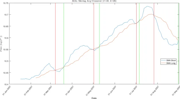
The moving average crossover rule uses two SMA’s, a short SMA and a longer SMA. A buy signal occurs when the faster (shorter) moving average crosses above the slower (longer) moving average, and a sell signal occurs when the shorter moving average crosses below the longer moving average.

Figure 1: Moving average crossover trading rule implemented on 8 months of Anglo American PLC (AGL) closing prices from 01-01-2007 to 30-08-2007. The log of the closing price (rather than just the closing price) is used for illustrative purposes. Green and red vertical lines represent buy and sell signals respectively.

3.1.2

Exponential Moving Average

The exponential moving average (EMA) makes use of today’s close price, yesterdays moving average value and a smoothing factor (α). The smoothing factor will determine how quickly the exponential moving average responds to current market prices [15]. A simple moving average is used for the initial EMA value.

3.1.2.1

Exponential Moving Average Crossover Rule

The calculation is identical to the Moving Average Crossover rule above however instead of using a SMA, an EMA is used.

3.1.2.2

EMA Indicator: EMA

(

n

)

EMA(Pc, n) =αP_tc+ (1−α)EMA(P_tc₋₁, n) (12) where α= 2

n+1

3.1.3

Highest High

Highest High is the greatest high price in the lastnperiods.

HH(n) = max(P_nh) (13)

3. TECHNICAL ANALYSIS

25

3.1.4

Lowest Low

Lowest Low is the smallest low price in the lastnperiods.

LL(n) = min(P_nl) (14)

where the vector with low prices of lastnperiods is given byP_nl = (Ptl−n, Ptl−n+1, Ptl−n+2, . . . , Ptl)

3.1.5

Ichimoku Kinko Hyo

The Ichimoku Kinko Hyo (at a glance equilibrium chart) system consists of five lines and the Kumo (cloud) [43,44, 45,46]. The five lines all work in concert to produce the end result. The size of the Kumo is an indication of the current market volatility, where a wider Kumo is a more volatile market.

3.1.5.1

Ichimoku Kinko Hyo Indicators

1. Tenkan-sen (Conversion Line): (HH(n1) + LL(n1))/2 2. Kijun-sen (Base Line): (HH(n2) + LL(n2))/2

3. Chikou Span (Lagging Span): Close plottedn2 days in the past 4. Senkou Span A (Leading Span A): (Conversion Line + Base Line)/2 5. Senkou Span B (Leading Span B):(HH(n3) + LL(n3))/2

6. Kumo (Cloud): Area between the Leading Span A and the Leading Span B form the Cloud

Ichimoku uses three key time periods for its input parameters: Typically,n1= 7, n2 = 22, and n3 = 44. We will keep the n1 parameter fixed at 7 but vary the other two look-back parameters n2 and n3. If the learning algorithm did have three free model parameters,n1could also be varied. We choose to fixn1since it impacts n the Conversion line which has the nearest correspondence to the closing price.

3.1.5.2

Ichimoku Kinko Hyo Strategies

The Kijun Sen Cross strategy is one of the most powerful and reliable trading strategies within the Ichimoku system due to the fact that it can be used on nearly all time frames with exceptional results [45].

Decision Condition

Buy Kijun Sen crosses the closing price curve from the bottom up

Sell Kijun Sen crosses the closing price curve from the top down

Hold otherwise

The buy and sell (bullish and bearish) signals are classified into three major classi-fications: strong, neutral and weak. The strength is determined by where the crossover occurs in relation to the cloud:

Strong:

buy, bullish cross happens above the kumo sell, bearish cross happens below the kumo Neutral:

buy, bullish cross happens within the kumo sell, bearish cross happens within the kumo Weak:

buy, bullish cross happens below the kumo sell, bearish cross happens above the kumo

Figure 2: Ichimoku Kijun Sen Cross strategy trading rule implemented on 9 months of Anglo American PLC (AGL) closing prices from 01-01-2007 to 30-09-2007. The log of the closing price (rather than just the closing price) is used for illustrative purposes. Green and red candle sticks refer to bullish and bearish trading days respectively. When the Leading span 1 is greater than the Leading span 2, the outlook is bullish (green cloud) and vice versa for a bearish outlook (red cloud). The number next to each of the vertical green and red lines indicate the strength of the buy and sell signals respectively.

3. TECHNICAL ANALYSIS

27

3.1.6

Momentum

3.1.6.1

Momentum Indicator: MOM

(

n

)

Momentum gives the change in the closing price over the past nperiods MOMt(n) =Ptc−P

c

t−n (15)

3.1.7

Momentum Trading Rule

Decision Condition

Buy MOMt−1(n) ≤ EMAt(MOMt(n), λ) & M OMt(n)> EM At(M OMt(n), λ)

Sell M OMt−1(n) ≥ EMAt(MOMt(n), λ) & MOMt(n)<EMAt(MOMt(n), λ)

Hold otherwise

Table 3: Momentum trading rule

3.1.8

Acceleration

3.1.8.1

Acceleration Indicator: ACC

(

n

)

Acceleration measures the change in momentum between two consecutive periods t andt−1

ACCt(n) = MOMt(n)−MOMt−1(n) (16)

3.1.8.2

Acceleration Trading Rule

Decision Condition

Buy ACCELt−1(n) + 1≤0 & ACCELt(n) + 1>0

Sell ACCELt−1(n) + 1≥0 & ACCELt(n) + 1<0

Hold otherwise

Table 4: Acceleration trading rule

3.1.9

Moving Average Convergence/Divergence Oscillator

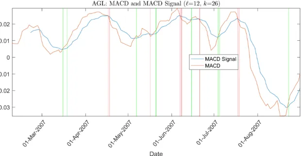
The Moving Average Convergence/Divergence (MACD) oscillator is a momentum in-dicator developed by Gerald Appel and attempts to determine whether traders are accumulating stocks or distributing stocks. It is calculated by computing the difference between a short-term and a long-term moving average. The idea is then to compute the signal line, which is accomplished by taking an exponential moving average of the MACD determines instances at which to buy (oversold) and sell (oversold) when used in conjunction with the MACD [11].

3.1.9.1

MACD Indicators: MACD

(

n

, n

)

1. LongEMA_t= EMAt(Pc, n2) 2. ShortEMAt= EMAt(Pc, n1)

3. MACDt(n1, n2) = ShortEMAt−LongEMAt

4. SignalLinet(n1, n2, n3) = EMAt(MACDt(n2, n1), n3)

5. MACDSt(n1, n2, n3) = MACDt(n1, n2)−SignalLinet(n1, n2, n3)

3.1.9.2

MACD Trading Rule

Decision Condition

Buy MACDt−1(n2, n1) ≤MACDSt(n2, n1, n3) & MACDt(n2, n1)>MACDSt(n2, n1n3)

Sell MACDt−1(n2, n1) ≥MACDSt(n2, n1, n3) & MACDt(n2, n1)<MACDSt(n2, n1, n3)

Hold otherwise

Table 5: MACD trading rule

Figure 3: MACD trading rule implemented on 9 months of Anglo American PLC (AGL) closing prices from 01-01-2007 to 30-08-2007. Green and red vertical lines represent buy and sell signals respectively.

3.1.10

Fast Stochastics

Fast stochastic oscillator shows the location of the closing price relative to the high-low range, expressed as a percentage, over a given number of periods as specified by

3. TECHNICAL ANALYSIS

29

a look-back parameter.

3.1.10.1

Fast Stochastic Indicators

Fast%Dt(n) = SMAt(Fast%Kt(n),3) (18)

3.1.10.2

Fast Stochastic Trading Rule

Decision Condition

Buy Fast%Kt−1(n) ≤ Fast%Dt(n) & Fast%Kt(n)>Fast%Dt(n)

Sell Fast%Kt−1(n) ≥ Fast%Dt(n) & Fast%Kt(n)<Fast%Dt(n)

Hold otherwise

Table 6: Fast stochastic trading rule

3.1.11

Slow Stochastics

The slow stochastic oscillator is very similar to the fast stochastic indicator in that it shows the location of the closing price relative to the high-low range over a given number of periods but only differs in the way that it is calculated. It is in fact just a moving average of the fast stochastic indicator. The fast stochastic indicator will typically be more sensitive to the closing price and will thus result in more frequent trading signals.

3.1.11.1

Slow Stochastic Indicators

Slow%Kt(n) = SMAt(Fast%Kt(n),3) (19) Slow%Dt(n):

Slow%Dt(n) = SMAt(Slow%Kt(n),3) (20)

3.1.11.2

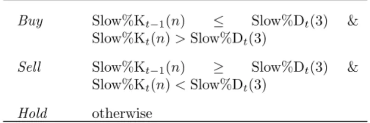
Slow Stochastic Trading Rule

Buy Slow%Kt−1(n) ≤ Slow%Dt(3) & Slow%Kt(n)>Slow%Dt(3)

Sell Slow%Kt−1(n) ≥ Slow%Dt(3) & Slow%Kt(n)<Slow%Dt(3)

Hold otherwise

Table 7: Slow stochastic trading rule

3.1.12

Relative Strength Index

Relative Strength Index (RSI) compares the periods that stock prices finish up (closing price higher than the previous previous) against those periods that stock prices finish down (closing price lower than the previous period) [9].

3.1.12.1

RSI Indicator: RSI

(

n

)

RSIt(n) = 100− 100 1 + SMAt(Pupn,n1) SMAt(Pdwnn ,n1) (21) where [9] P_tup= ( Pc t ifPtc−1< Ptc NaN otherwise (22) P_tdwn= ( Pc t ifPtc−1> Ptc NaN otherwise (23) and P_nup = (P_tup_−n, P_tup_−n+1, . . . , P_tup) (24) P_ndwn= (P_tdwn_−n, P_tdwn_−n+1, . . . , P_tdwn) (25)

3.1.12.2

RSI Trading Rule

Decision Condition

Buy RSIt−1(n)≤30 & RSIt(n)>30

Sell RSIt−1(n)≥70 & RSIt(n)<70

Hold otherwise

3. TECHNICAL ANALYSIS

31

Figure 4: RSI trading rule implemented on 9 months of Anglo American PLC closing prices from 01-01-2007 to 30-08-01-01-2007. Green and red vertical lines represent buy and sell signals respectively.

3.1.13

Moving Average Relative Strength Index

Moving Average Relative Strength Index (MARSI) is an indicator that smooths out the action of RSI indicator [47].

3.1.13.1

MARSI Indicator: MARSI

(

n

, n

)

MARSI is calculated by simply taking ann2-period SMA of the RSI indicator. MARSIt(n1, n2) = SMA(RSIt(n1), n2) (26)

3.1.13.2

MARSI Trading Rule

Rather buying or selling when RSI crosses upper and lower thresholds (30 and 70) as in the RSI trading rule above, buy and sell signals are generated when the SMA of the MARSI crosses above or below the thresholds [47].

Decision Condition

Buy MARSIt−1(n)≤30 & MARSIt(n)>30

Sell MARSIt−1(n)≥70 & MARSIt(n)<70

Hold otherwise

3.1.14

Bollinger Band

Bollinger bands uses a SMA (Bollm_t (n)) as it’s reference point (known as the median band) with regards to the upper and lower Bollinger bands denoted by Bollu_t(n) and Bolld_t(n) respectively and are calculated as functions of standard deviations (s). When the closing price crosses above (below) the upper (lower) Bollinger band, it is a sign that the market is overbought (oversold) [9].

3.1.14.1

Bollinger Band Indicator: Boll

(

n

)

Upper Bollinger band: Bollm_t (n) +sσ2_t(n) Lower Bollinger band: Bollm_t (n)−sσ_t2(n)

(27)

where sis typically chosen to be 2.

3.1.14.2

Bollinger Trading Rule

Decision Condition Buy Pc t−1≥Boll d t(n) & Ptc ≥Boll u t(n)

Sell P_tc₋₁≤Boll_td(n) & P_tc >Bollu_t(n)

Hold otherwise

Table 10: Bollinger trading rule

3.1.15

Price Rate-Of-Change

3.1.15.1

PROC Indicator: PROC

(

n

)

The rate of change of the time series of closing prices Pc

t over the last n periods expressed as a percentage PROCt(n) = 100· Pc t −Ptc−n Pc t−n (28)

3.1.15.2

PROC Trading Rule

Decision Condition

Buy PROCt−1(n)≤0 & PROCt(n)>0

Sell PROCt−1(n)≥0 & PROCt(n)<0

Hold otherwise

3. TECHNICAL ANALYSIS

33

3.1.16

Williams %R

3.1.16.1

Williams %R Indicator: Will

(

n

)

Williams Percent Range (Williams %R) is calculated similarly to the fast stochastic oscillator and shows the level of the close relative to the highest high in the last n periods

Willt(n) =

HH(n)−Pc t

HH(n)−LL(n)·(−100) (29)

3.1.16.2

Williams %R Trading Rule

Decision Condition

Buy Willt−1(n)≥ −20 & Willt(n)<−80

Sell Willt−1(n)≤ −20 & Willt(n)>−80

Hold otherwise

Table 12: Williams %R trading rule

3.1.17

Parabolic SAR

Parabolic Stop and Reverse (SAR), developed by J. Wells Wilder, is a trend indicator formed by a parabolic line made up of dots at each time step [48]. The dots are formed using the most recent Extreme Price and an acceleration factor (AF), 0.02, which increases each time a new Extreme Price (EP) is reached. The AF has a maximum value of 0.2 to prevent it from getting too large. Extreme Price represents the highest (lowest) value reached by the price in the current up-trend (down-trend). The acceleration factor determines where in relation to the price the parabolic line will appear by increasing by the value of the AF each time a new EP is observed and thus affects the rate of change of the Parabolic SAR.

3.1.17.1

SAR Indicator: SAR(

n

)

The steps involved in calculating the SAR indicator are as follows:

1. initialise variables: trend is initially set to 1 (up-trend), EP to zero,AF0to 0.02, SAR0to the closing price at time zero (Pc

0), lastHigh to high price at time zero (Ph

0) and lastLow to the low price at time zero (P0l))

2. update parameters: EP, lastHigh, lastLow and AF based on where the current high is in relation to the lastHigh (up-trend) or where the current low is in relation to the lastLow (down-trend)

3. compute the next period SAR value: update time t+ 1 SAR value, SARt+1, using Eq. (30)

4. modify the SAR value and the parameters for a change in trend: modify the SARt+1 value, AF, EP lastLow, lastHigh and the trend based on the trend and its value in relation to the current lowPl

t and current highP0h 5. go to next time period and return to step 2

Below is the formula for the Parabolic SAR for timet+ 1 calculated using the previous value at timet:

SARt+1= SARt+α(EP−SARt) (30)

3.1.17.2

SAR Trading Rule

Decision Condition

Buy SARt−1≥Ptc−1 & SARt< Ptc

Sell SARt−1≤Ptc−1 & SARt> Ptc

Hold otherwise

Table 13: SAR trading rule

3.2

Trend Following and Contrarian Mean

Rever-sion Strategies

The zero-cost BCRP (trend following), zero-cost anti-BCRP and zero-cost anti-correlation (both contrarian mean-reverting) algorithms are explained in more detail in the fol-lowing subsections.

3.2.1

Zero-Cost BCRP

Zero-cost BCRP is the zero-cost (long/short and self-financing) version of the BCRP strategy and is a trend following algorithm in that long positions are taken in stocks during upward trends while short positions are taken during downward trends. The idea is to first find the portfolio controls that maximise the expected utility of wealth using all in-sample price relatives according to a given constant level of risk aversion. The resulting portfolio equation is what is known to be the Mutual Fund Separation Theorem [40]. The second set of portfolio controls in the mutual fund separation theorem (active controls) is what we will use as the set of controls for the zero-cost BCRP strategy and are given by:

b= 1 γΣ −1 E[R]−11 |_Σ−1 E[R] 1|Σ−1₁ (31) where Σ−1_{is the inverse of the covariance matrix of returns for allmstocks,}

E[R]

is vector of expected returns of the stocks,1is a vector of ones of lengthmandγ is the risk aversion parameter. Eq. (31) is the risky Optimal Tactical Portfolio (OTP) that takes optimal risky bets given the risk aversionγ. The risk aversion is selected during each periodtsuch that the controls are unit leverage and hence Pm

i |bi|= 1. The covariance matrix and expected returns for each periodtare computed using the set of price relatives from today back`days (short-term look-back parameter).

3.2.2

Zero-Cost Anti-BCRP

Zero-cost anti-BCRP is exactly the same as zero-cost BCRP except that we reverse the sign of the expected returns vector such thatE[R] =−E[R].