An experimental testbed for mobile offshore base control concepts
Anouck R. Girard, Daniel M. Empey, William C. Webster, and J. Karl HedrickOcean Engineering Graduate Group, The University of California at Berkeley, 230 Bechtel Engineering Center #1708, Berkeley, CA 94720-1708, USA
a self-propelled, floating, prepositioned base that would accept cargo from aircraft and container ships, and dis-charge resources to the shore via a variety of surface vessels and aircraft.2 All platforms would provide per-sonnel housing, equipment maintenance functions, ves-sel and lighterage cargo transfer, and logistic support for rotary wing and short take-off aircraft. The longest platform assembly (nominally 2 km in length) would also accommodate conventional take-off and landing (CTOL) aircraft, including the Boeing C-17 cargo trans-porter.3 In short, the MOB would act somewhat like an aircraft carrier, but on a much larger physical scale. The MOB is not expected to reach its destination at high speeds, or in one piece.
The effort of the University of California, Berkeley (UCB), and the California Partners for Advanced Transit and Highways (PATH) Program is part of the MOB technical base effort devoted to determining the feasibility of the dynamic positioning of multiple MOB platforms, as described by Remmers et al.2 In this project we have developed an automated multimodule dynamic positioning control system for the MOB, and a simulation template for uniform support of dynamic positioning (DP) control systems during tests and evalu-ations. The virtual demonstration consisted of the simu-lation of several different MOB control methods under a range of environmental conditions, and we compared control system performances using an evaluation toolkit that was also developed during the project. The inter-ested reader is referred to Sousa et al.4 and Girard et al.5 In this project, the team was also required to validate the key design issues physically with scale models of the MOB. This paper will be concerned with a description of the physical experiments that have been conducted to date using the set-up. The next four sections present an overview of the MOB control experimental facility, and the fundamental control concepts for the MOB, the actual control laws used, and a discussion of scaling effects. The final part discusses the results obtained
Abstract The concept of a mobile offshore base (MOB) reflects the need to stage and support military and humani-tarian operations anywhere in the world. A MOB is a self-propelled, modular, floating platform that can be assembled into lengths of up to 2 km, as required, to provide logistic support to US military operations where fixed bases are not available or adequate. It accommodates the take-off and landing of C17 aircraft, and can be used for storage, as well as to send resources quickly to shore. In most concepts, the structure is made of three to five modules, which have to perform long-term station-keeping in the presence of winds, waves, and currents. This is usually referred to as dynamic positioning (DP). In the MOB, the alignment is maintained through the use of thrusters, connectors, or a combination of both. In this paper, we consider the real-time control of scaled models of a MOB. The modules are built at the 1 : 150 scale, and are kept aligned by rotating thrusters under a hierarchical hybrid control scheme. This paper describes a physical testbed developed at the University of California, Berkeley, under a grant from the US Office of Naval Research, for the purpose of evaluating competing MOB control concepts.
Key words Dynamic positioning · Mobile offshore base · Ex-perimental validation · Real-time control system
Introduction
A mobile offshore base (MOB) is intended to provide a forward presence anywhere in the world. It serves as the equivalent of land-based assets, but is situated closer to the area of conflict and is capable of being relocated. In operation, it would be stationed far enough out to sea to be defended easily.1 As presently envisioned, a MOB is
Address correspondence to: A.R. Girard
(e-mail: [email protected])
from the physical experiment comparing different MOB control concepts.
Control concepts for the MOB
In order to support air and sea operations, the MOB is required to:
1. be assembled at sea;
2. remain aligned and assembled to allow for the land-ing of aircraft and cargo transfer from ships; 3. be aligned into the wind to facilitate the landing of
aircraft;
4. be disassembled if the environmental conditions become too severe or in case of emergency.
There are several different control problems to be dealt with in order to have successful MOB operations. The first is the assembly of the modules forming the MOB at sea. Because of its size and because it must be mobile, the MOB will be composed of independent platforms/modules, and will be assembled at or near the point of deployment. Each of these modules can be expected to be of the order of 100–400m long, and perhaps 50–100 m wide. Bringing two such dynamically independent modules together and joining them at sea will be a nontrivial operation. Obviously the modules will have to separate at the end of the mission. In general, this is a much simpler problem than the assem-bly, but could be a difficult maneuver under emergency conditions.
Station-keeping is clearly an important problem for the MOB. Dynamic positioning, or DP, where a ship/ platform must remain (on the surface) within a certain radius of a point on the sea floor, has been tackled by the oil industry to maintain oil platforms over the drill hole. Traditionally, either mooring lines or thruster units are used to counter environmental forces. For a MOB, mooring lines are not attractive, as the runway must be aligned into the wind at all times for planes to land with maximum control. Also, unlike an oil plat-form, the exact position of the assembled MOB with respect to the Earth is not of paramount importance, as the runway will continue to function satisfactorily even if it drifts, and the pilots will be able to see the structure from above.
One of the most important characteristics for a MOB will be that is kept runway straight and flat. This governs the ability of aircraft to take off and land. The positions of the MOB modules must be controlled very tightly relative to their neighbors, while the assembly as a whole must maintain a reasonable position with respect to the sea floor. This allows for a reduction in power consumption (cost) in lower sea states, and focuses all the control effort on maintaining the relative alignment
in high sea states. As an assembly, it must be possible for the MOB to be aligned into the wind under its own power.
Control law
The breadth of maneuvers to be controlled and the difficulties inherent to the ocean environment being somewhat daunting to address in one step, the control strategy was organized into hierarchical layers. This is a standard approach for the control of complex, net-worked systems of vehicles, and hierarchical control approaches have been applied with great success to the control of autonomous underwater vehicles, au-tonomous helicopters, and intelligent vehicle highway systems, among others.6
The lowest level of the hierarchy controls the scaled thrusters, and limits them with software to the equiva-lent behavior of the full-scale units. The behavior of the units was determined by experimental testing, the scaled thrusters were built in-house, and look-up tables were used to control the thrusters using a power-based approach.7 As environmental disturbances in the ocean are likely to come from any direction, the thrusters on each module pivot so that they can produce force and moment systems in all directions.
Once the individual thrusters have been dealt with, the next layer in the hierarchy is called thruster allocation logic (TAL). This considers the number of thrusters on the module, their characteristics, and, given a desired force and moment system on the platform, uses linear programming techniques to optimize the thrust and azimuth angle that each individual thruster must produce. TAL has been shown to result in fuel economies, and also allows the designer to take thruster failure into account directly by simply informing the TAL that one or more of the thrusters has new charac-teristics. The interested reader is referred to Webster and de Sousa.8
The coordinated DP layer receives the desired posi-tion for the MOB, and the desired relative spacing for the neighboring modules, and determines the force and moment that must be applied on the MOB to achieve the alignment and global position goals in the best pos-sible way. There are several pospos-sible approaches to de-signing the DP law for the modules. We have chosen to use a nonlinear control method called dynamic surface control (DSC). A typical solution used by the industry is a linear control technique called proportional–integral– derivative (PID) control. The advantages of using non-linear vs. non-linear control methods are that nonnon-linearities in the dynamics of the platform can be taken into account directly by the nonlinear controller. In addi-tion, we can guarantee properties of stability and
robustness in the DSC approach. Finally, multiinput, multioutput systems can be considered, and can be tuned naturally using DSC. DSC is a control technique that is similar to integrator back-stepping, but which uses first-order filters to alleviate the classical explosion of terms problem. Model uncertainty can be dealt with directly. An outline of the derivation of the control law is presented here. For further information, including the proof of stability and robustness, and a more complete comparison with other control methods, the reader is referred to Girard.9
The equations of motion of a platform when derived in their complete form are very complex, not only because of the sheer number of equations and forces, but also because the hydrodynamic force models are complex. In this section, we present a low-frequency model of the platform dynamics that was implemented and used for the controller design. This model describes the motions of the dynamically positioned system.
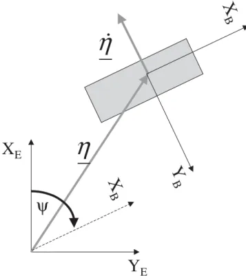
The motion of the body-fixed frame is described rela-tive to an inertial frame. The inertial frame is denoted (XE, YE, ZE), where the subscript E stands for earth-fixed. Typically, the inertial frame is chosen so that XE points north, YE points east, and ZE points down toward the center of the Earth. Now consider the 2D problem. In the (XE, YE, ZE) frame, the platform has a position vector h, with components [x, y, y], where x and y designate the position, and y is the heading angle. In the inertial frame, a velocity vector h˙ can also be defined
with components [x. y.y.].
The position and the velocity are vectors, and can be expressed in any basis. When thinking about vehicles, it is convenient to define a body-fixed frame, say (X, Y, Z). The Society of Naval Architects and Marine Engineers (SNAME) has dictated standards for choos-ing the body-frame, so that the X-position is directed from aft to fore, the Y-position is directed to starboard, and Z is pointing downward, as shown in Fig. 1.
A free-floating body in the ocean moves in all six degrees of freedom. In the dynamic positioning of vessels, we want to control a vessel (or platform) on the ocean surface with respect to the ocean floor. This is because dynamic positioning is traditionally used to connect an oil well on the sea floor with a vessel on the surface using a pipeline. Dynamic positioning vessels are not generally equipped with actuators in heave, roll, or pitch. We consider the two-dimensional problem where we deal with the surge (XB-position), sway (YB-position), and yaw (rotation about ZB) motions.
The equations of motion which describe the low-frequency motion of a surface vessel can be written in the body-fixed frame as10
Mv C v v D v v˙+
( )
+( )
= +t tenv (1) h˙ =J( )
hv (2) where:— = [u r]T is formed from the body-fixed
com-ponents of the Earth-fixed velocity vector of the platform;
— h. = [x. y. y.]T is the velocity of the platform in the
inertial frame;
— M is the mass plus added mass matrix of the plat-form (from the physical standpoint, the added mass represents the amount of fluid accelerated with the body);
— C() is the Coriolis and centripetal matrix; — D() is the damping matrix;
— t represents the body-fixed forces from the actuators;
— tenv represents viscous drag and forces due to the environment (wind, waves, and currents);
— J(h) is a transformation matrix between the inertial and body-fixed coordinate frames, with
J h y y y y
( )
=( )
-( )
( )
( )
È Î Í Í Í ˘ ˚ ˙ ˙ ˙ cos sin sin cos 0 0 0 0 1 (3)In these equations we have assumed zero current velocity as a simplification for the controller design.
h
X
EY
Eh
y
X
BY
BX
BFig. 1. Inertial (earth-fixed) and body-fixed frames for the derivation of the equations of motion
Also, the equations are in two dimensions (i.e., we consider three degrees of freedom). The thrusters only counteract the “horizontal” forces and act in surge, sway, and yaw. The “vertical” motions, heave (ZB-position), roll (rotation about XB), and pitch (rotation about YB), are not considered here. For conventional ships and platforms, rolling and pitching motions have zero mean and limited amplitude.
The total motion of the ship in waves is given by the sum of a low-frequency component and the wave-frequency motion. The low-wave-frequency component is separated out from the total measured ship motions by a wave filtering system. Attempting to control the oscil-latory motion due to the waves causes wear and tear on the thrusters, and in general actuator bandwidth is insufficient to counter those motions efficiently. Several filters, as well as a nonlinear observer, have been devel-oped for filtering these motions.9
Nonlinear control of one vessel
The control problem is to choose the actuator forces to be applied so that the vessel reaches the desired inertial coordinates hd =
[
x yd d d]
T , ,Y (4)The DSC controller involves two “sliding surfaces.” The first surface defines the desired vessel position and orientation. The second surface defines the desired velocity which, if maintained, will drive the vessel to the desired position. Thruster forces are chosen so that the second surface approaches zero.
The first surface is defined as s1= -h hd (5) Differentiating s1 yields s˙1=J
( )
hv-h˙d (6) At this point, the desired velocity, or “synthetic con-trol,” d is defined as
J
( )
hvd =h˙d -L1 1s (7) where L1 is a positive definite matrix. With this defini-tion, if =d, then
˙s1= -L1 1s (8) and s1Æ 0 with a convergence rate determined by the choice of L1. Because of the definition of s1, this will also guarantee that hÆhd.
The second sliding surface can be defined as s2 = -d, but computing the derivative of s2 could lead to a very complex control law. A method called dynamic
surface control (DSC), and described by Swaroop et al.,11 eliminates the need for model differentiation. First, we pass d through a bank of first-order filters:
Tz z˙+ =vd (9)
where T is a diagonal matrix whose elements, Tii, are the
filter time constants. These are chosen to be as small as possible, consistent with numerical conditioning problems. “z” now serves as an estimate of d, with a derivative that is easily computed as
˙z T= -1
(
vd -z)
(10)Using z in place of d, we now define the second sliding surface as
s2= -v z (11)
At this point, a Lyapunov approach can be used. We select the Lyapunov function candidate to be
V s Ms T =1 2 2 2 (12)
Differentiating V and using Eqs. 1 and 11 yields
V˙ =s Mv MzT2
[
˙- ˙]
=sT2[
tT-C v v Mz( )
- ˙]
(13) where tT, the thruster force, is considered to be the only force acting on the vessel for the purpose of controller design. If tT is selected as
tT =C v v Mz K s
( )
+ ˙- D 2 (14) where KD is a positive, definite, symmetric gain matrix, then
V˙ = -s K sT2 D 2 (15)
which guarantees that s2Æ 0. This in turn implies that Æd, s1 Æ 0, and hÆhd. Using Eq. 10, the control law can be written in terms of z as
tT =C v v MT
( )
+ -1(
vd-z)
-K sD 2 (16) Control of multiple vesselsThere are a great number of different possible strategies for coordinating MOBs. The goal of every strategy is to position the vessels in a straight line with tight relative spacing constraints. Three control strategies have been tested and implemented (Hedrick et al. 1999), using either the first or the middle modules as leaders in follow-the-leader-type algorithms, or using leader-less control where each module tracks an inertial reference and maintains a desired relative spacing with respect to
the other modules. The best results were produced by this last approach using
1st vessel: s11=h1-h1d+Lr
(
h1-h2-h12d)
(17) 2 12 2 2 1 2 3 nd vessel: d2 d21 d23 s r r = - +(
- -)
+(
- -)
h h h h h h h h L L (18) 3rd vessel: s13=h3-h3d+Lr(
h3-h2-h32d)
(19) where hdij is the desired relative spacing between modules i and j. The above notation allows us to see clearly the interactions of the two separate terms, with the first part of each s1 surface dealing with tracking an inertial position, and the second part dealing with adjustments to the relative position. One reason to separate both terms so explicitly is that for the MOB, the absolute position of the assembled platforms does not have tight requirements, as pilots can easily see the structure from the air, or receive a radio message giving the exact position of the floating runway. However, fuel economy is a significant issue, and the assembled MOB should be allowed to drift within reason. The relative alignment of the platforms is of paramount importance for landing planes. The two-tiered control laws, as pre-sented in Eqs. 17–19, allow us to make this distinction clear. If one only uses absolute positions, fuel consump-tion may be higher than is necessary. If one only con-trols relative platform positions, the assembly may drift significantly.By adjusting the diagonal elements of Lr, the impor-tance of absolute vs. relative errors can be changed, with higher values corresponding to tighter relative position accuracy. Some of the attractive features of this approach are: (1) there is guaranteed string stability,12 since each vessel has an inertial reference, and (2) an identical control structure can be used for both decoupled and coupled maneuvers. If it is desired to decouple the vessels and send them to arbitrary loca-tions, then Lr ∫ 0 and hdi is defined for each separate vessel. By coupled, we mean that the modules are tioned in relation to their neighbors (coordinated posi-tioning), and by decoupled we mean that the modules are positioned independently of one another.
Goals of model testing and scaling effects
Because no one has experience of actually constructing and operating a MOB, the need to perform model tests during the various phases of the design process is more crucial that during the design of a conventional ship.
During the design of the MOB, a model of the behavior of the modules was required in order to select and optimize the various elements of the controller.
Simulation was used, since it is impractical and overly time-consuming to expect to validate each variation in the design using model tests. To have reasonable confidence in the simulation tools, the behavior of the modules must be predicted adequately, in particular with respect to changes in performance with minor variations. The simulation tool developed during the project was called MOB–SHIFT, and the interested reader is referred to Sousa et al.4 An important engi-neering goal of the experiments has been to confirm that all of the important hydrodynamic phenomena have been identified and captured in MOB–SHIFT. This was accomplished by careful comparisons of the MOB–SHIFT behavior predictions with the perfor-mance of the experimental models. This has allowed us to use MOB–SHIFT simulations with confidence to evaluate particular control system designs for the MOB through exhaustive simulation in a variety of environ-mental conditions and for a variety of operational scenarios.
One of the questions that is always evoked during the planning and construction of physical models is that of scaling. Test-basin considerations limit the range of possible scales to somewhere between 1 : 100 and 1 : 200. Dimensional analysis, through the use of the Buckingham-pi theorem,10 guarantees that the physics for a model experiment will match that of the full-scale situation if and only if the dimensionless parameters formed from all of the governing variables are matched exactly. In practice, this condition is nearly impossible to meet, as it requires conflicting values for many of the test parameters. In particular, fixing the Froude number for the MOB guarantees that the physics of wave action at the model scale is identical to that at full scale; match-ing the Reynolds number is functionally impossible for MOB testing, at the scales considered. On a small-scale model, it is impossible to model the viscous effects (Reynolds number) and wave effects (Froude number) simultaneously. Further, because of the lack of viscous and surface-tension effects, scale-model thrusters do not perform like full-scale thrusters if the scaling calls for too small a thruster diameter. As a result, one usu-ally needs to compromise between model scale (larger is better) and cost (costs for both construction and testing increase drastically with size).
When choosing the model scale for our experiment, we considered the purpose of the experiment, the vis-cous drag forces, the handling of the model, the model function, and the size of the test facility. In the first phase, we built relatively small models (1 : 150 scale). This choice allowed us to float three scaled MOB modules in the Berkeley basin, which were large enough to carry the appropriate control computers, thrusters, and actuators. A model of this size is just large enough to be tested in a basin, and to avoid major surface tension
and capillary wave problems. There are drawbacks to models this small, of course, with the main issues being propeller (thruster) scaling and viscous drag forces. As mentioned above, scaled thrusters do not perform like full-scale thrusters if the viscous effects are not scaled, and scaling the viscous effects properly is functionally impossible. For our experiments, the thruster is approxi-mately 4.7cm in diameter, and thrust characterization (i.e., thrust versus propeller r.p.m.) does not scale up correctly. However, the thrusters have been designed to have the correct scaled azimuth control (rotation speed and accuracy), and the correct thrust time constants. The only thing that does not scale correctly is the thrust to propeller r.p.m. curve. This means that the thruster/ thruster and thruster/hull interactions may not be the same as those in a full-scale module, and that the lowest-level control law for the scaled thruster would not be applicable to the full-scale units. Viscous drag forces are more difficult to characterize, but ship models are almost universally tested in water, and theoretical methods exist for correcting the model scale results for the viscosity of water. In our case, the problem was slightly simpler as the MOB modules do not move through the water at any appreciable speed, and the effects due to improper scal-ing of the Reynolds number are greatly reduced.
The models built at Berkeley are small scale (1: 150), economical models and have been designed to capture the basic hydrodynamic performance of the MOB modules, and to allow a representative performance of the thrusters. The purpose of the models was to confirm that all of the relevant hydrodynamic parameters had been captured in MOB–SHIFT, along with a demon-stration of MOB control techniques for at-sea assembly of modules, multimodule dynamic positioning, align-ment into the wind, and the separation of modules. This has given credibility to the overall MOB concept. All of the above goals have been met. Here, we will concen-trate on the validation of control maneuvers.
The Berkeley test basin does not allow for the generation of repeatable disturbances. Although distur-bances were introduced at times for visual effect, in general, experiments in the basin did not include envi-ronmental disturbances. MOB–SHIFT was used to test the behavior of the MOB modules in control algorithms in severe environmental conditions. The interested reader is referred to Girard et al.5
MOB control testbed
The PATH program at UCB has developed a 1 : 150-scale physical model of a generic mobile offshore base (MOB). This concept utilizes three or more indepen-dently operable deep-sea-going semsubmersible plat-forms that are used in conjunction with one another to
create a stable sea-based runway for large cargo and other aircraft. The model consists of three 1.80-m ¥ 0.76-m independent floating “0.76-modules,” each equipped with four controllable (azimuth and thrust) thrusters and sensors that provide both inertial and relative-position information. The models are operated in a 16-m ¥ 30-m ¥
0.75-m-deep tank, located at the UCB, Richmond Field Station. The system is controlled by a real-time com-puter system located at the side of the tank.
Scaled MOB modules
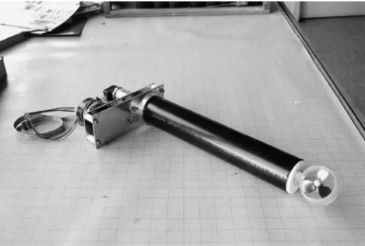
The heart of the MOB physical model is the 1: 150-scale module, constructed from closed-cell foam, acrylic plas-tic, and aluminum tubing. The scale module is base on a full-sized “generic” module developed by researchers at the US Naval Academy. The scale module is 1.8m long, 0.76 m wide, has a draft of about 20 cm, and weighs close to 90 kg. One module is shown in Fig. 2. Each module is equipped with four variable-thrust, dirigible, ducted propellers, one mounted on each “corner.” These thrusters were designed and made at UCB and provide a true scale representation of the actual thrusters that would be used on full-scale modules (Fig. 3). The thrusters are electrically powered, with d.c. servomotors providing the variable thrust, while stepper motors control the azimuth.
Visually, the most impressive feature of the models is the thruster indicator mounted on top of each of the thrusters (Fig. 4). When in operation, a red LED “bar-graph” indicates the direction and magnitude of the thruster force vector. The tests are videotaped from above, and the indicators allow the video to be used as a first-order-of-magnitude check of the system’s func-tion. The indicators also give a quick visual reference as to what each module is doing, and are quite useful for trouble-shooting.
The modules are equipped with both absolute and relative position sensors. The absolute position sensor system consists of a laser beacon/position transponder system using two “shore”-mounted rotating laser bea-cons, with two position transponders on each module. This system measures the position of the transponders relative to the fixed beacon baseline on the side of the tank. Because there are two transponders on each boat, the position and orientation of each module can be determined in a inertial coordinate system. The accu-racy of the system is approximately ± 2 cm.
The relative position measuring system consists of six ultrasonic sensors, three for each “gap” between the modules, which measure both the longitudinal and the lateral separation of the modules. The accuracy of this system is about ±2 mm.
Computer control system
The scale modules are controlled from the “shore” of the tank by a network of computers. The control signals
are passed to the modules via overhead “umbilical” cables, one to each module. The computer control sys-tem is composed of four computers, one that interfaces directly with the hardware, and three that run the com-plex control algorithms (Fig. 5). The interface computer is equipped with digital and analog I/O boards that connect to the modules via the umbilical cables; this computer, in turn, is connected to the other three puters with serial and Ethernet links. All of the com-puters run the QNX real-time operating system. Test facility
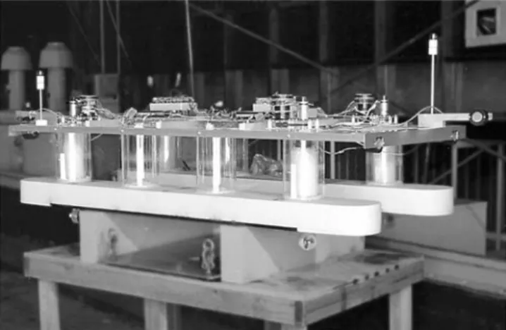
The system is operated in a large indoor tank about 16 m ¥ 30 m ¥ 0.75 m deep (Fig. 6). This facility allows the testing of small-scale models in the absence of external disturbances such as wind, but also provides
Fig. 3. Scaled thruster for the MOB control experiment
Fig. 4. Thruster indicator
Fig. 5. Computer control system
Fig. 6. University of California at Berkeley test facility. Three modules are being operated from the bridge. The central com-puter is located on the bridge, and the umbilical cables that connect the central computer to the modules are visible in the picture
the opportunity to inject known disturbances into the system and measure the response.
Experimental results
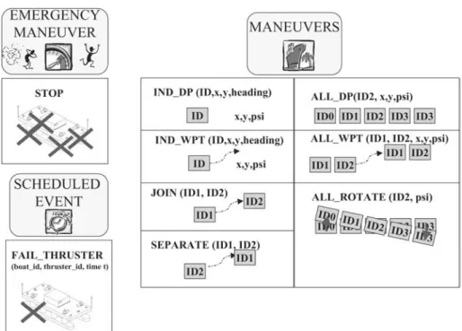
The user interface for the experiment includes a menu offering a choice of several maneuvers. A maneuver coordinates the motion of one or several modules; legal maneuvers are shown in Fig. 7. These include moving one module to a new position and heading, assembling modules to form a bigger MOB, separating assembled modules, moving a string of modules to a new position and heading, and rotating a string of modules into the wind.
A typical mission would include dynamic positioning at the initial location, bringing the modules into widely spaced positions in a straight line, docking the modules to form a string, performing coordinated station-keeping (DP), rotating the string through 10° and bring-ing it back, performbring-ing a coordinated lateral maneuver, and separating the modules. A full run takes about 20–30min. A video showing all these maneuvers can be obtained from the PATH web page:
http://www.path.berkeley.edu
under the Publications and Video heading, or from the author’s home page:
http://path.berkeley.edu/~anouck/mob2.html
For the purposes of this paper, we present logged data from an actual experiment. The data from the com-plete mission is difficult to interpret visually, so we
con-Fig. 7. Legal maneuvers in the experimental setup
centrate on the DP, docking, and coordinated rotation parts of the scenario.
Figure 8 is an x/y plot of a module station-keeping in the tank. It shows the motions of the center of gravity of the module in the x and y directions. The x and y posi-tions are given in meters, so the movements of the cen-ter of gravity of the boat are of the order of +/-2 cm in either the x or the y direction, which is about the accuracy of the absolute measurement system.
10.14 10.15 10.16 10.17 5.485 5.49 5.495 5.5 5.505 5.51 x position in meters y position in meters
x/y plot of module 1 during coordinated DP
Fig. 8. x position (in meters) vs. y position (in meters) of the center of gravity of one module while performing dynamic positioning at a set point (10.15, 5.5)
Figure 9 is a plot of the heading angle of the module shown in Fig. 8 during the same period of time. The desired heading angle is 0°.
At the start of a mission, the modules usually station-keep for some time, and then assemble. The assembly maneuver is split into two parts. First, the modules
350 400 450 500 550 600 -1 -0.8 -0.6 -0.4 -0.2 0 0.2 0.4 0.6 0.8 1 time in seconds
heading angle in degrees
heading angle of module 1 during coordinated DP
Fig. 9. Heading angle of the module shown in Fig. 8 (in degrees), vs. time (in seconds), also while performing dynamic positioning. The angle is maintained within +/-1° of its desired value
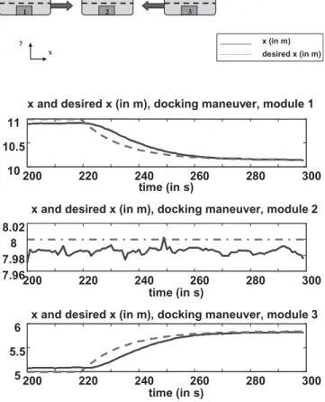
1 1 22 33 y x x (in m) desired x (in m) 200 220 240 260 280 300 10 10.5 11
x and desired x (in m), docking maneuver, module 1
200 220 240 260 280 300
7.96 7.98 8 8.02
x and desired x (in m), docking maneuver, module 2
200 220 240 260 280 300
5 5.5
6
x and desired x (in m), docking maneuver, module 3 time (in s)
time (in s)
time (in s)
Fig. 10. x position of the modules (in meters) vs. time while performing a precision docking maneuver
Fig. 11. Heading angles of all three modules (in degrees) vs. time (in seconds) during a coordinated rotation maneuver from 0° to 5°
move into a straight line while remaining far apart. Then the two end modules come in and dock precisely. Figure 10 shows the x locations of the three modules being used in a precision docking maneuver. Module 1 is shown in the upper plot, module 2 is in the center, and module 3 is in the lower plot. The desired positions are shown by dashed lines, and the actual positions by solid lines. Initially, modules 1 and 3 are not in exactly the desired position because of umbilical forces. Module 2 station-keeps during the whole maneuver.
Finally, Fig. 11 shows the actual and desired heading angles for all three modules during a coordinated rota-tion maneuver. The heading angle is shown in degrees (vs. time in seconds), and the desired maneuver called for a rotation from 0° to 5°. The actual response lags behind the desired heading angle, but the alignment between all the modules is tightly maintained at all times.
Conclusions
This paper describes a testbed for dynamic positioning control strategies for the mobile offshore base that was developed at the University of California, Berkeley, and California PATH between 1998 and 2001.
The MOB control testbed was presented, control strategies for the MOB were discussed, and experimen-tal results were provided.
Early experimental results obtained using the testbed have been encouraging. Improvements to the testbed could be made in two directions: the modules should be made with no wires to extend their range and get rid of the forces exerted by the umbilical cables, and the testbed would greatly benefit from an improved abso-lute position system.
Acknowledgments. This material is based on work sup-ported by the MOB Program of the US Office of Naval Research under grant N00014-98-1-0744. The authors would like to thank the Link Foundation for its support. Many thanks go to Stephen Spry for his experimental work. The photographs are courtesy of Bill Stone, Gerald Stone, and Jay Sullivan of the PATH Publica-tions staff.
References
1. Zueck R, Palo P, Taylor R (1999) Mobile offshore base: research spin-offs. Proceedings of the 1999 ISOPE Conference, Brest, France, vol 10, p 16
2. Remmers G, Taylor R, Palo P, et al (1999) Mobile offshore base: a sea-basing option. Keynote Address, International Workshop on Very Large Floating Structures, VLFS ’99, vol 1, p 7 3. Polky J (1999) Airfield operational requirements for a mobile
offshore base. International Workshop on Very Large Floating Structures, vol 1, pp 206–219
4. Sousa J, Girard A, Kourjanskaia N (1998) The MOB–shift simulation framework. International Workshop on Very Large Floating Structures, vol 1, pp 474–482
5. Girard A, Borges de Sousa J, Hedrick K (2001) Simulation envi-ronment design and implementation: an application to the mobile offshore base. Offshore Mechanics and Arctic Engineering Conference, OMAE01, vol 5, pp 1–9
6. Girard A, Borges de Sousa J, Hedrick K (2001) An overview of emerging results in networked multi-vehicle systems. IEEE Conference on Decision and Control, CDC01, vol 1, pp 432– 437
7. Spry S, Empey D, Webster W (2001) Design and characterization of a small-scale azimuthing thruster for a mobile offshore base module. Mar Struct J 14:215–229
8. Webster J, Borges de Sousa J (1999) Optimum allocation for multiple thruster. Proceedings of the 1999 ISOPE Conference, Brest, France, vol 83, p 89
9. Girard A (2002) Hybrid system formalisms for coordinated vehicle control. PhD Dissertation, Ocean Engineering Graduate Group, University of California at Berkeley
10. Newman J (1977) Marine hydrodynamics. MIT, Cambridge 11. Swaroop D, Hedrick K, Yip P, et al (2001) Dynamic surface
control for a class of nonlinear systems. IEEE Trans Autom Control 45:1893–1899
12. Swaroop D, Hedrick K (1996) String stability of interconnected systems. IEEE Trans Autom Control 41:349–357