HAL Id: hal-02320543
https://hal.archives-ouvertes.fr/hal-02320543
Submitted on 21 Oct 2019
HAL
is a multi-disciplinary open access
archive for the deposit and dissemination of
sci-entific research documents, whether they are
pub-lished or not. The documents may come from
teaching and research institutions in France or
L’archive ouverte pluridisciplinaire
HAL
, est
destinée au dépôt et à la diffusion de documents
scientifiques de niveau recherche, publiés ou non,
émanant des établissements d’enseignement et de
recherche français ou étrangers, des laboratoires
On agnostic post hoc approaches to false positive control
Gilles Blanchard, Pierre Neuvial, Etienne Roquain
To cite this version:
Gilles Blanchard, Pierre Neuvial, Etienne Roquain. On agnostic post hoc approaches to false positive
control. 2019. �hal-02320543�
On agnostic post hoc approaches to
false positive control
Gilles Blanchard
Universit¨at Potsdam, Institut f¨ur Mathematik Karl-Liebknecht-Straße 24-25 14476 Potsdam, Germany
Laboratoire de Math´ematiques d’Orsay, Universit´e Paris-Sud, CNRS,
Universit´e Paris-Saclay, 91405 Orsay Cedex, France e-mail:[email protected]
Pierre Neuvial
Institut de Math´ematiques de Toulouse; UMR 5219, Universit´e de Toulouse, CNRS UPS IMT, F-31062 Toulouse Cedex 9, France e-mail:[email protected]
Etienne Roquain
Sorbonne Universit´e, Laboratoire de Probabilit´es, Statistique et Mod´elisation, LPSM, 4, Place Jussieu, 75252 Paris cedex 05, France
e-mail:[email protected]
Abstract: This document is a book chapter which gives a partial survey on post hoc approaches to false positive control.
Contents
1 Setting and basic assumptions . . . 2
2 From confidence bounds ... . . 2
3 ... to post hoc bounds . . . 3
4 Threshold-based post hoc bounds . . . 6
5 Reference families . . . 9
6 Case of a fixed single reference set . . . 11
7 Case of spatially structured reference sets . . . 12
8 Applications . . . 13
8.1 Confidence envelopes . . . 14
8.2 Data-driven sets . . . 15
8.3 Structured reference sets . . . 16
9 Bibliographical notes . . . 18
Acknowledgements . . . 19
Classical approaches to multiple testing grant control over the amount of false positives for a specific method prescribing the set of rejected hypotheses. On the other hand, in practice many users tend to deviate from a strictly pre-scribed multiple testing method and follow ad-hoc rejection rules, tune some parameters by hand, compare several methods and pick from their results the one that suits them best, etc. This will invalidate standard statistical guarantees because of the selection effect. To compensate for any form of such ”data snoop-ing”, an approach which has garnered significant interest recently is to derive ”user-agnostic”, or post hoc, bounds on the false positives valid uniformly over all possible rejection sets; this allows arbitrary data snooping from the user. In this chapter, we start from a common approach to post hoc bounds taking into account the p-value level sets for any candidate rejection set, and explain how to calibrate the bound under different assumption concerning the distribution of p-values. We then build towards a general approach to this problem using a family of candidate rejection subsets (call this a reference family) together with associated bounds on the number of false positives they contain, the latter holding uniformly over the family. It is then possible to interpolate from this reference family to find a bound valid for any candidate rejection subset. This general program encompasses in particular thep-value level sets considered ini-tially in the chapter; we illustrate its interest in a different context where the reference subsets are fixed and spatially structured. These methods are then applied to a genomic example of differential expression study. In this chapter, all references are gathered in Section9.
1. Setting and basic assumptions
Let us observe a random variable X with distribution P belonging to some model P. Consider mnull hypotheses H0,i ⊂ P,i ∈Nm ={1, . . . , m}, forP.
We denoteH0(P) ={i∈Nm : P satisfiesH0,i}the set of true null hypotheses
and H1(P) = Nm\H0(P) its complement. We assume that a p-value pi(X) is
available for each null hypothesisH0,i, for eachi∈Nm.
We introduce the following assumptions on the distribution P, that will be useful in the sequel:
∀i∈ H0(P), ∀t∈[0,1], P(pi(X)≤t)≤t; (Superunif) {pi(X)}i∈H0(P)is a family of indep. variables, indep. of{pi(X)}i∈H1(P).
(Indep)
2. From confidence bounds ...
Consider some fixed deterministicS ⊂ Nm. A (1−α)-confidence bound V =
V(X) for|S∩ H0(P)|, the number of false positives inS, is such that
∀P ∈ P, PX∼P
A first example is given by thek0-Bonferroni boundV(X) =Pi∈S1{pi(X)≥αk0/|S|}+ k0−1,for some fixedk0∈Nmsuch thatk0≤ |S|(otherwise the bound is trivial).
The coverage probability is ensured under (Superunif) by the Markov inequality: P(|S∩ H0(P)| ≥V + 1) ≤P |S∩ H0(P)| ≥ X i∈S∩H0(P) 1{pi(X)≥αk0/|S|}+k0 =P X i∈S∩H0(P) 1{pi(X)< αk0/|S|} ≥k0 ≤ |S∩ H0(P)|αk0/|S| k0 ≤α.
However, in practice,S is often chosen by the user and possibly depends on the same data set, then denotedSbto emphasize this dependence; it typically
corresponds to items of potential strong interest. The most archetypal example is whenSbconsists of thes0 smallestp-values p(1:m), . . . , p(s0:m), for some fixed
value of s0 ∈Nm. In that case, it is easy to check that the above bound does
not have the correct coverage: for instance, when thep-values are i.i.d.U(0,1) andH0(P) =Nm, we have fork0≤s0(that is, when the bound is informative),
P(|Sb∩ H0(P)| ≤V) =P k0−1 +Pi∈Sˆ1{pi(X)≥αk0/s0} ≥s0 =P P i∈Sˆ1{pi(X)< αk0/s0} ≤k0−1 =P p(k0:m)(X)≥αk0/s0 =P(β(k0, m−k0+ 1)≥αk0/s0),
whereβ(k0, m−k0+ 1) denotes the usual beta distribution with parametersk0 andm−k0+ 1. For instance, takings0= 10,k0= 5,α= 0.05 andm= 500, the latter is approximately equal to 0.005, while the intended target is 1−α= 0.95. This phenomenon is often referred to as the selection effect: after some data driven selection, the probabilities change and thus the usual statistical inferences are not valid.
3. ... to post hoc bounds
To circumvent the selection effect, one way is to aim for a function V(X,·) : S⊂Nm7→V(X, S)∈N(denoted byV(S) for short) satisfying
∀P ∈ P, PX∼P
∀S⊂Nm, |S∩ H0(P)| ≤V(S)
≥1−α, (1)
that is, a (1−α) confidence bound that is valid uniformly over all subsets S ⊂ Nm. As a result, for any particular algorithm S, inequality (b 1) entails
P |Sˆ∩ H0(P)| ≤ V( ˆS)≥ 1−α, and thus does not suffer from the selection effect. Such a bound will be referred to as a (1−α)-post hoc confidence bound
throughout this chapter, ”post hoc” meaning that the setScan be chosen after having seen the data, and possibly using the data several times.
As a first example, thek0-Bonferroni post hoc boundis
Vk0 Bonf(S) =|S| ∧ X
i∈S
1{pi(X)≥αk0/m}+k0−1
!
. (2)
Following the same reasoning as above, it has a coverage at least 1−αunder (Superunif): P(∃S⊂Nm : |S∩ H0(P)| ≥Vk0 Bonf(S) + 1) ≤P ∃S⊂Nm : X i∈S∩H0(P) 1{pi(X)< αk0/m} ≥k0 ! =P X i∈H0(P) 1{pi(X)< αk0/m} ≥k0 ! ≤ |H0(P)|αk0/m k0 ≤α.
Remark 0.1 Compared to the k0-Bonferroni confidence bound of Section2,α
has been replaced byα|S|/m, so that the post hoc bound is much more conserva-tive than a (standard, non uniform,S fixed) confidence bound when|S|/mgets small, which is well expected. This scaling factor is the price paid here to make the inference post hoc. We will see in Sections4and7that it can be diminished when considering bounds of a different nature.
Exercise 0.1 Fork0= 1, when thep-values are i.i.d.U(0,1)andH0(P) =Nm,
prove that the coverage probability of thek0-Bonferroni post hoc bound is at most (1−α/m)m. Does the Bonferroni post hoc bound provide a sharp coverage in
that case?
The Bonferroni post hoc bound, while it is valid under no assumption on the dependence structure of the p-value family, may be conservative, in the sense thatV(S) will be large for many subsetsS. For instance, one hasVk0 Bonf(S) =
|S|(trivial bound) for all the setsS such thatS⊂ {i∈Nm : pi(X)> αk0/m}. The Bonferroni bound can be further improved under some dependence re-striction, with theSimes post hoc bound:
VSim(S) = min 1≤k≤|S| ( X i∈S 1{pi(X)≥αk/m}+k−1 ) = min 1≤k≤|S|{V kBonf(S)}. (3)
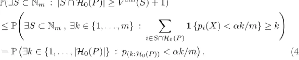
Its coverage can be computed as follows (using arguments similar as above): P(∃S ⊂Nm : |S∩ H0(P)| ≥VSim(S) + 1) ≤P ∃S⊂Nm, ∃k∈ {1, . . . , m} : X i∈S∩H0(P) 1{pi(X)< αk/m} ≥k ! =P ∃k∈ {1, . . . ,|H0(P)|} : p(k:H0(P))< αk/m . (4)
Under (Superunif) and (Indep), this is lower than or equal to α|H0(P)|/m≤α by using the Simes inequality. More generally, the Simes post-hoc bound is valid in any setting where the Simes inequality holds. This is the case under a specific positive dependence assumption called Positive Regression Dependency on a Subset of hypotheses (PRDS), which is also the assumption under which the Benjamini-Hochberg (BH) procedure has been shown to control the false discovery rate (FDR).
While it uses more stringent assumptions,VSim(S) can be much less
conser-vative thanVk0 Bonf. For instance, ifS={i∈
Nm : 5α/m≤pi(X)<10α/m},
we haveV5Bonf(S) =|S|andVSim(S)≤ |S| ∧9, which can lead to a substantial
improvement.
From Exercise0.2below, the Simes bound has a nice graphical interpretation: |S| −VSim(S) can be interpreted as the smallest integerufor which the shifted
linev7→α(v−u)/mis strictly below the ordered p-value curve, see Figure1.
● ●● ● ● ● ● ● ● ● ● ● ● ● ● ● ● ● ● ● 0 5 10 15 20 0.00 0.05 0.10 0.15 0.20 ● ● ● ● ● ● ● ● ● ● ● ● ● ● ● ● 0 5 10 15 20 0.00 0.05 0.10 0.15 0.20
Fig 1. Illustration of the Simes post hoc bound (3)according to the expression (5), for two subsets ofNm(left display/right display), both of cardinal20and form= 50. The level isα=
0.5(taken large only for illustration purposes). Black dots: sortedp-values in the respective subsets. Lines: thresholdsk∈ {u+ 1, . . . ,|S|} 7→α(k−u)/m(in red foru=|S| −V(S), in light gray otherwise). The post hoc boundVSim(S)corresponds the length of the bold line on
theX-axis.
Exercise 0.2 Prove that for allS ⊂Nm,|S| −VSim(S) is equal to
where p(1:S), . . . , p(|S|:S) denote the ordered p-values of {pi(X), i ∈ S}. [Hint:
start from|S| −VSim(S)≤ufor someu, and find equivalent expressions.]
Exercise 0.3 In Figure1, check thatVSim(S) = 18(resp.VSim(S) = 12) in the
left (resp. right) situation. Compare toVk0Bonf fork
0= 7 (m= 50,α= 0.5). The Simes post hoc bound (3) has, however, several limitations: first, the coverage is only valid when the Simes inequality holds. This imposes restrictive conditions on the model used, which are rarely met or provable in practice. Sec-ond, even in that case, the bound does not incorporate the dependence structure, which may yield conservativeness (see Exercise0.4 below). Finally, this bound intrinsically compares the orderedp-values to the thresholdk7→αk/m(possibly shifted). We can legitimately ask whether taking a different threshold (called template below) does not provide a better bound.
Exercise 0.4 Consider the caseH0(P) =Nm, for whichmis even, and denote
Φthe upper-tail distribution function of a standard N(0,1) variable. Consider the one-sided testing situation wherepi= Φ(X1),1≤i≤m/2andpi= Φ(X2), m/2+1≤i≤m, for a2-dimensional Gaussian vector(X1, X2)that is centered,
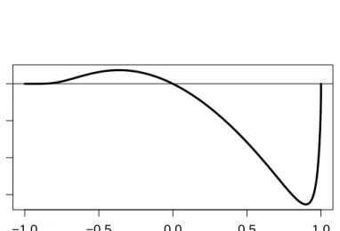
with covariance matrix having 1 as diagonal elements and ρ ∈ [−1,1] as off-diagonal elements. Show that the coverage probability of the Simes post hoc bound is equal to α/2 + Z α α/2 Φ Φ −1 (α)−ρΦ−1(w) (1−ρ2)1/2 ! dw+ Z ∞ α Φ Φ −1 (α/2)−ρΦ−1(w) (1−ρ2)1/2 ! dw (6)
The above quantity is displayed in Figure2forα= 0.2, as a function of ρ.
4. Threshold-based post hoc bounds
More generally, let us consider bounds of the form
Vλ(S) = min 1≤k≤|S| ( X i∈S 1{pi(X)≥tk(λ)}+k−1 ) , λ∈[0,1], (7)
wheretk(λ),λ∈[0,1], 1≤k≤m, is a family of functions, called a template.
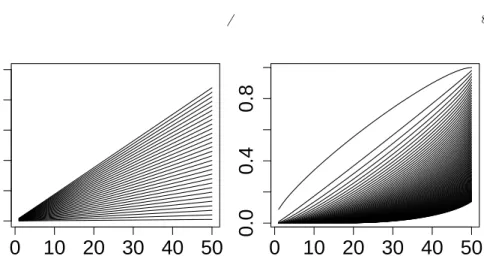
A template can be seen as a spectrum of curves, parametrized byλ. We focus here on the two following examples:
• Linear template:tk(λ) =λk/m,t−k1(y) =ym/k;
• Beta template:tk(λ) =λ-quantile ofβ(k, m−k+ 1),t−k1(y) =P(β(k, m−
k+ 1)≤y).
An illustration for the above templates is provided in Figure3.
For a fixed template, the idea is now to choose one of these curves, that is, one value of the parameterλ=λ(α), so that the overall coverage is larger than
−1.0 −0.5 0.0 0.5 1.0
0.17
0.18
0.19
0.20
Fig 2. Coverage of the Simes post hoc bound(6)in the setting of Exercise0.4as a function ofρand forα= 0.2.
1−α. Following exactly the same reasoning as the one leading to (4), we obtain P(∃S⊂Nm : |S∩ H0(P)| ≥Vλ(S) + 1) ≤P ∃k∈ {1, . . . ,|H0(P)|} : p(k:H0(P)) < tk(λ) (8) =P min k∈{1,...,|H0(P)|} t−k1(p(k:H0(P))) < λ , (9)
by lettingt−k1(y) = max{x∈[0,1] : tk(x)≤y}the generalized inverse oftk (in
general, this is valid provided that for allk ∈ {1, . . . , m}, tk(0) = 0 and tk(·)
is non-decreasing and left-continuous on [0,1], as in the case of the two above examples). What remains to be done is thus to calibrateλ=λ(α, X) such that the quantity (9) is belowα.
Several approaches can be used for this. It is possible that for the model under consideration, the joint distribution of (pi(X))i∈H0(P) is equal to the
restriction of some known, fixed distribution on [0,1]Nm to the coordinates of
H0(P) (this is a version of the so-called subset-pivotality condition). It is met under condition (Indep), but it is also possible that the dependence structure of thep-values is known (for example, in genome-wide association studies, the structure and strength of linkage disequilibrium can be tabulated from previ-ous studies and give rise to a precise dependence model). In such a situation, the calibration of λ =λ(α, X) can be obtained either by exact computation, numerical approximation or Monte-Carlo approximation under the full null.
Another situation of interest, on which we focus for the remainder of this sec-tion, is when the null corresponds to an invariant distribution with respect to a
0
10 20 30 40 50
0.0
0.4
0.8
0
10 20 30 40 50
0.0
0.4
0.8
Fig 3. Curves k 7→ tk(λ) for a wide range of λ values. Left: linear template. Right: beta template.
certain group of data transformations, which is the setting for (generalized) per-mutation tests, allowing for the use of an exact randomization technique. More precisely, assume the existence of a finite transformation groupG acting onto the observation setX. By denotingpH0(x) the nullp-value vector (pi(x))i∈H0(P)
forx∈ X, we assume that the joint distribution of the transformed nullp-values is invariant under the action of anyg∈ G, that is,
∀P ∈ P, ∀g∈ G, (pH0(g
0.X))
g0∈G ∼(pH0(g0.g.X))g0∈G, (Rand) whereg.X denotesX that has been transformed byg.
Let us consider a (random)B−tuple (g1, g2, . . . , gB) ofG (for some B ≥2),
whereg1is the identity element ofG andg2, . . . , gBhave been drawn
(indepen-dently of the other variables) as i.i.d. variables, each being uniformly distributed onG. Now, let for allx∈ X, Ψ(x) = min1≤k≤mt−k1 p(k:m)(x) and consider λ(α, X) = Ψ(bαBc+1) where Ψ(1) ≤ Ψ(2) ≤ · · · ≤ Ψ(B) denote the ordered sample (Ψ(gj.X),1≤j≤B). The following result holds.
Theorem 0.1 Under (Rand), for any deterministic template, the boundVλ(α,X)
is a post hoc bound of coverage1−α. This level is to be understood as a joint probability with respect to the data and the draw of the group elements(gi)2≤i≤B.
As a case in point, let us consider a two-sample framework where X = (X(1), . . . , X(n1), X(n1+1), . . . , X(n1+n2))∈(
Rm)n
is composed of n = n1+n2 independent m-dimensional real random vectors with X(j), 1 ≤ j ≤ n
1, i.i.d. N(θ(1),Σ) (case) and X(j), n1+ 1 ≤ j ≤ n, i.i.d. N(θ(2),Σ) (control). Then we aim at testing the null hypotheses H
0,i :
“θi(1) =θ(2)i ”, simultaneously for 1≤ i ≤m, without knowing the covariance matrix Σ. Consider any family of p-values (pi(X))1≤i≤m such thatpi(X) only
depends on thei-th coordinate (Xi(j))1≤j≤n of the observations (e.g., based on
difference of the coordinate means of the two groups). Note thatpH0(X) is thus
a measurable function of (Xi(j))i∈H0,1≤j≤n. Now, the groupG of permutations
of {1, . . . , n} is naturally acting on X = (Rm)n via the permutation of the individuals: for allσ∈ G,
σ.X= (X(σ(1)), . . . , X(σ(n1)), X(σ(n1+1)), . . . , X(σ(n))).
Exercise 0.5 Show that(Xi(1))i∈H0, . . . ,(X
(n)
i )i∈H0 are i.i.d. and prove(Rand).
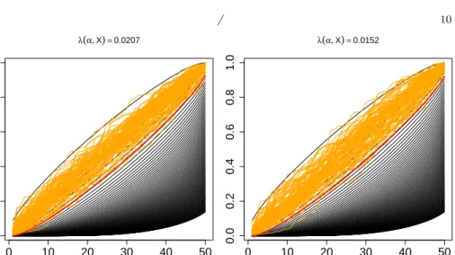
An illustration of the aboveλ-calibration method is provided in Figure4 in the case where Σ =Im,
pi(X) = 2 1−Φ s −1 n1,n2 n−21 n1+n2 X j=n1+1 Xi(j)−n−11 n1 X j=1 Xi(j) ! , forsn1,n2 = (n −1 1 +n −1
2 )1/2 and using a beta template. In the left panel (full null), we haveθ(1)=θ(2)= 0, so thatH0(P) =
Nm. In the right panel (half of
true nulls), we haveθi(1)=θ(2)i = 0 for 1≤i≤m/2 andθ(1)i = 0,θi(2)=δ/sn1,n2
form/2 + 1≤i≤m, for some δ >0, so thatH0(P) ={1, . . . , m/2}. Following expression (8), k 7→ tk(λ(α, X)) is the highest beta curve such that at most
Bα orange curves have a point situated below it. This also shows that the above λ-calibration is slightly more severe when part of the data follows the alternative distribution. This is a commonly observed phenomenon: although the permutation approach is valid even when part of the null hypotheses are false, their inclusion in the permutation procedure tends to yield test statistics that exhibit more variation under permutation, thus inducing more conservativeness in the calibration.
5. Reference families
We cast the previous bounds in a more general setting, where (1−α)–post hoc bounds are explicitly based on areference familywith somejoint error rate(JER in short) controlling property. This general point of view offers more flexibility and allows us to consider post hoc bounds of a different nature, as for instance those incorporating a spatial structure, see Section7.
In general, a reference family is defined by a collectionR= (R1(X), ζ1(X)), . . . ,(RK(X), ζK(X)), where theRk’s are data-dependent subsets ofNm and
theζk’s are data dependent integer numbers (we will often omit the dependence
in X to ease notation). The reference family R is said to control the JER at levelαif
∀P ∈ P, PX∼P(∀k∈NK : |Rk(X)∩ H0| ≤ζk(X))≥1−α. (10)
Markedly, (10) is similar to (1), but restricted to some subsetsRk,k∈NK. The
0 10 20 30 40 50 0.0 0.2 0.4 0.6 0.8 1.0 λ(α, X)=0.0207 0 10 20 30 40 50 0.0 0.2 0.4 0.6 0.8 1.0 λ(α, X)=0.0152
Fig 4. Illustration of the λ=λ(α, X)calibration method on one realization of the dataX. Black curves: beta templatek7→tk(λ)for some range ofλ values. Orange curves: ordered p-values (after permutation) k 7→ p(k:m)(gj.X) for 1 ≤ j ≤ B = 1000. Red curve:k 7→ tk(λ(α, X)). Left panel : full null, right panel : half of true nulls (see text). (Parameters
m= 50,α= 0.2,n1= 50,n2= 50,δ= 3.)
free in (1) (to accommodate any choice of the practitioner), the choice of the Rk’s and ζk’s in (10) is done by the statistician and is part of the procedure.
Once we obtain a reference familyRsatisfying (10), we obtain a post hoc bound by interpolation:
VR∗(S) = max{|S∩A| : A⊂Nm,∀k∈NK,|Rk∩A| ≤ζk}, S⊂Nm. (11)
We call VR∗ the optimal post hoc bound (built upon the reference family R). Computing the boundVR∗(S) can be time-consuming, it actually has NP-hard complexity in a general configuration. We can introduce the following com-putable relaxations: forS⊂Nm,
VR(S) = min k∈NK (|S\Rk|+ζk)∧ |S|; (12) e VR(S) = X k∈NK |S∩Rk| ∧ζk+ S\ [ k∈NK Rk ! ∧ |S|. (13)
Exercise 0.6 Show that VR∗(S)≤VR(S)andVR∗(S)≤VeR(S)for all S⊂Nm.
Moreover, provided that (10) holds, show that VR∗, VR and VeR are all valid (1−α)–post hoc bounds.
In addition, the following result shows that the relaxed versions coincide with the optimal bound if the reference sets have some special structure:
Lemma 0.1
• In the nested case, that is, Rk ⊂ Rk+1, for 1 ≤ k ≤ K−1, we have VR=VR∗;
• In the disjoint case, that is,Rk∩Rk0 =∅ for1 ≤k6=k0 ≤K, we have e
VR=VR∗.
We can briefly revisit the post-hoc bounds of the previous sections in this general framework. Thek0-Bonferroni post hoc bound (2) derives from the one-element reference family (R = {i∈Nm:pi(X)< αk0/m}, ζ = k0−1). The Simes post hoc bound (3) derives from the reference family comprising the latter reference sets for allk0 ∈Nm. More generally, the threshold-based post
hoc boundsVλ of the form (7) are equal to the optimal bound VR∗ withRk = {i∈Nm : pi(X)< tk(λ)}and ζk =k−1,k∈Nm(indeed, these reference sets
are nested, so thatVR∗ =VR).
How to choose a suitable reference family in general? A general rule of thumb is to choose the reference setsRk of the same qualitative form as the setsS for
which the bound is expected to be accurate. For instance, the Simes post hoc bound will be more accurate for setsS with the smallestp-values. In Section7, we will choose reference setsRk with a spatial structure, which will produce a
post hoc bound more tailored for spatially structured subsetsS.
6. Case of a fixed single reference set
It is useful to focus first on the case of a single fixed (non-random) reference set R1, with (random)ζ1 satisfying (10), that is,
P(|H0(P)∩R1| ≤ζ1(X))≥1−α.
(In contrast with thek0-Bonferroni bound (2) whereζwas fixed andRvariable, hereR1is fixed andζ1is variable.) In other words,ζ1(X) is a (1−α)–confidence bound of|H0(P)∩R1|. Several example of suchζ1(X) can be build, under various assumptions.
Exercise 0.7 ForR1⊂Nm fixed, show that the following bounds are (1−α)–
confidence bounds for|H0(P)∩R1|:
• under (Superunif), for some fixedt∈(0, α),
ζ1(X) =|R1| ∧ $ X i∈R1 1{pi(X)> t}/(1−t/α) % , (14)
where bxc denotes the largest integer smaller than or equal to x. [Hint: use the Markov inequality.]
• under (Superunif)and (Indep),
ζ1(X) =|R1|∧min t∈[0,1) $ C 2(1−t)+ C2 4(1−t)2 + P i∈R11{pi(X)> t} 1−t 1/2%2 , (15) where C = q 1 2log 1 α
. [Hint: use the DKW inequality, that is, for any integern≥1, forU1, . . . , Un i.i.d.U(0,1), we haven−1P
n
i=11{Ui> t} −
(1−t)≥ −p
In addition to the two above bounds (14) and (15), we can elaborate another bound in the generalized permutation testing framework (Rand), as described in Section 4. Applying the result of that section, the following bound is also valid: ζ1(X) = min 1≤k≤|R1| ( X i∈R1 1{pi(X)≥tk(λ(α, X))}+k−1 ) , (16) where tk(λ) denotes the λ-quantile of a β(k,|R1| −k+ 1) distribution and λ(α, X) = Ψ(bαBc+1), where Ψ(1) ≤ Ψ(2) ≤ · · · ≤ Ψ(B) denote the ordered sample (Ψ(gj.X),1≤j≤B) for which Ψ(x) = min1≤k≤|R1|
t−k1 p(k:|R1|)(x)
(see theλ-calibration method of Section 4).
Once a proper choice ofζ1(X) has been done, the optimal post hoc bound can be computed as follows: for any S ⊂ Nm, VR∗(S) = VR(S) = VeR(S) = |S∩R1c|+ζ1(X)∧ |S∩R1|.WhenS is large and does not contain very small p-values, this bound can be sharper than the Simes bound.
Exercise 0.8 Let us consider a post bound based on the single reference family
R1 =Nm and ζ1(X)as in (15) (choosing t= 1/2). ForS such that S ⊂ {i∈
Nm : pi(X)> α|S|/m}, show thatVSim(S) =|S| and VR∗(S) = |S| ∧ζ1(X)≤ |S| ∧2 log 1 α + 2P i∈Nm1{pi(X)>1/2} .
Finally, while the case of a single reference set can be considered as an el-ementary example, the bounds developed in this section will be useful in the next section, for which several fixed reference setsRk are considered, and thus
several (random)ζk should be designed.
7. Case of spatially structured reference sets
We consider here the case where the null hypothesesH0,i, 1 ≤i≤m, have a
spatial structure, and we are interested in obtaining accurate bounds on|S∩ H0(P)| for subsets S of the form S = {i ∈ Nm : i0 ≤ i ≤ j0}, for some 1≤i0< j0≤m.
In that case, it is natural to chooseRk formed of contiguous indices. To be
concrete, consider reference sets consisting of disjoint intervals of the same size : assumem=Ksfor some integersK >0 ands >0 and let
Rk ={(k−1)s+ 1, . . . , ks}, k∈NK. (17)
When each of these regions is considered in isolation, Section6suggested several approaches (in the appropriate settings (Superunif), (Indep) or (Rand)) of a specific formζk(X) =f(Rk, α, X), to underline the dependence of ζk(X) inRk
andα. By using a simple union bound, it is then straightforward to show that the JER control (10) is satisfied for
When the reference regionsRk are disjoint as in the example (17) above, we
can use the proxyVeR(S) (see (13)) which is known to coincide with the optimal boundVR∗(S). This gives rise to a post hoc bound that accounts for the spatial structure of the data.
Exercise 0.9 Compute ζk(X) in the case where ζ1(X) =f(R1, α, X)is given
by (14) (t = α2) and (15). In each case, for a given k, discuss how ζk(X)
fluctuates when the size of the familyK increases.
When considering the reference regions defined by segments (17), we have to prescribe a scale (shere, the size of the segments). It is possible to extend this to a multi-scale approach, choosing overlapping reference intervalsRk at different
resolutions arranged in a tree structure, where parent sets are formed by taking union of (disjoint) children sets taken at a finer resolution. Furthermore, the proxy (13) has to be replaced by a more elaborate one, minimizing over all possible multi-scale partitions made of such reference regions. This can still be computed efficiently by exploiting the the tree structure. Doing so, the post hoc bound will be more scale adaptive to setsSwith possibly various sizes. The price to pay lies in the cardinalityK of the family, which gets larger. However, this does not necessarily make the corresponding bound much larger, as Exercise0.9
shows when using the bound (15), since the levelαonly enters it logarithmically.
8. Applications
Differential gene expression studies in cancerology aim at identifying genes whose mean expression level differs significantly between two (or more) cancer populations, based on a sample of gene expression measurements from individ-uals from these populations. We consider here a microarray data set1consisting
of expression measurements for more than 12,000 genes for biological samples from n = 79 individuals with B-cell acute lymphoblastic leukemia (ALL). A subset of cardinaln1= 37 of these individuals harbor a specific mutation called BCR/ABL, while the remainingn2 = 42 don’t. One of the goals of this study is to identify those genes for which there is a difference in the mean expression level between the mutated and non-mutated population. This question can be addressed, after relevant data preprocessing, by performing a statistical test of equality in means for each gene. A classical approach is then to derive a list of “differentially expressed” genes (DEG) as those passing a FDR correction by the Benjamini-Hochberg (BH) procedure at a user-defined level. For example, 163 genes are selected by the BH procedure at levelα= 0.05. We note that al-though the usage of the BH procedure is standard for multiple two-sample tests and widely accepted in the biomedical literature, we have no formal guarantee that it is mathematically justified – in particular, genes are not independent, and there is no proof that the PRDS assumption holds in this setting.
In this section, we illustrate how the post hoc inference framework introduced in the preceding sections can be applied to this case to build confidence envelopes
for the proportion of false positives (Section8.1), and to obtain bounds on data-driven sets of hypotheses (Section8.2), and on sets of hypotheses defined by an a priori structure (Section8.3). These numerical results were obtained using the R packagesansSouci, version 0.8.12.
8.1. Confidence envelopes
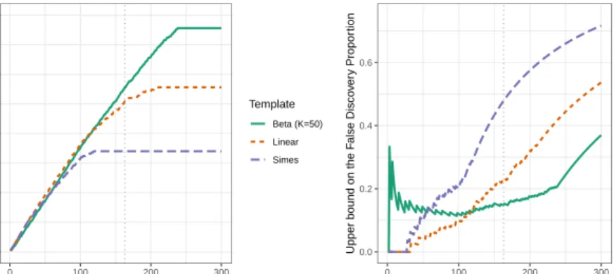
In absence of specific prior information on relevant subsets of hypotheses to con-sider, it is natural to focus on subsets consisting of the most significant hypothe-ses. Specifically, we define thek−thp-value level setSk as the set of thekmost
significant hypotheses, corresponding to thep-values (p(1:m), p(2:m), . . . , p(k:m)), and consider post hoc bounds associated to Sk for k ∈ Nm. Figure 5
pro-vides post hoc confidence envelopes for the ALL data set, for α = 0.1. While (1−α)-lower confidence bounds on the number of true positives of the form
k,|Sk| −V(Sk)
:k∈Nm are displayed in the left panel, (1−α)-upper
con-fidence bounds on the proportion of false positives
k, V(Sk)/|Sk|
:k∈Nm
are shown in the right panel.
The confidence envelopes are built from the Simes bound (3) (long-dashed purple curve), and from two bounds obtained from Theorem0.1byλ-calibration usingB= 1,000 permutation of the sample labels, based on the two templates introduced in Section4: the dashed red curve corresponds to the linear template withK=m, and the solid green curve to the beta template withK= 50. Note that Assumption (Rand) holds because we are in the two-sample framework de-scribed after Theorem0.1. The vertical line in Figure5 corresponds to the 163
0 50 100 150 200 0 100 200 300
Number of selected genes
Lo w er bound on the n umber of tr ue disco v er ies Template Beta (K=50) Linear Simes 0.0 0.2 0.4 0.6 0 100 200 300
Number of selected genes
Upper bound on the F
alse Disco v er y Propor tion Template Beta (K=50) Linear Simes
Fig 5. Confidence bounds on the number of true positives (left) and on the proportion of false
positives (right) for several reference families: Simes reference family (long-dashed purple curve), linear template after λ-calibration (dashed red curve), and beta template after λ -calibration (solid green curve).
genes selected by the BH procedure at level 5%. The Simes bound ensures that 2Available fromhttps://github.com/pneuvial/sanssouci.
the FDP of this subset is not larger than 0.48. As noted above concerning the BH procedure, we have a priori no guarantee that this bound is valid, because such multiple two-sample testing situations have not been shown to satisfy the PRDS assumption under which the Simes inequality is valid3. In contrast, the
λ-calibrated bounds built by permutation are by construction valid here. More-over, both are much sharper than the Simes bound while theλ-calibrated bound using the linear template is twice smaller, ensuring FDP<0.23, and even smaller for the beta template withK= 50. The bound obtained byλ-calibration of the linear template is uniformly sharper that the original Simes bound (3), which corresponds to λ =α. This illustrates the adaptivity to dependence achieved byλ-calibration. The bound obtained from the beta template is less sharp for p-value level sets Sk of cardinal less than k = 120, and then sharper. This is
consistent with the shape of the threshold functions displayed in Figure3.
8.2. Data-driven sets
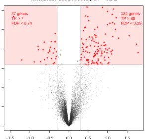
A common practice in the biomedical literature is to only retain, among the genes called significant after multiple testing correction, those whose “fold change” exceeds a prescribed level. The fold change is the ratio between the mean ex-pression levels of the two groups. With the notation of Section 4, the fold-change of geneiis given by ∆i=X
(2) i /X (1) i , whereX (1) i =n −1 1 Pn1 j=1X (j) i and X(2)i =n−21Pn2 j=1X (j) i .
This is illustrated by Figure6, where each gene is represented as a point in the (log(fold change),−log(p)) plan. This representation is called a “volcano plot” in the biomedical literature. Among the 163 genes selected by the BH procedure at level 0.05, 151 have an absolute log fold change larger than 0.3. As FDR is not preserved by selection, FDR controlling procedures provide no statistical guarantee on such data-driven lists of hypotheses. In contrast, the post hoc bounds proposed in this chapter are valid for such data-driven sets. The two shaded boxes in Figure6 correspond to the data-driven subsetsSBH∩S− and SBH∩S+, whereSBH is the set of 163 genes selected by the BH procedure at level 0.05,S−={i∈
Nm,log(∆i)<−0.3}andS+={i∈Nm,log(∆i)>+0.3}.
The post hoc bounds on the number of true positives inSBH∩S+, SBH∩S− and SBH∩(S+ ∪S−) obtained by the Simes bound and by the λ-calibrated linear and beta templates are given in Table8.2. Bothλ-calibrated bounds are more informative than the Simes bound, in the sense that they provide a higher bound on the number of true confidence. Moreover, they have proven (1− α)-coverage, whereas the coverage of the Simes bound is a priori unknown for multiple two-sample tests. None of the twoλ-calibrated bounds dominates the other one, which is in line with the fact that the linear template is well-adapted to situations with smallerp-value level sets than the beta template.
Finally, we also note that the bound obtained forS+∪S− is systematically 3In this particular case,λ-calibration with the linear template yieldsλ(α)> α, which a posteriori implies that the Simes inequality was indeed valid.
● ● ● ● ● ● ● ● ● ● ● ● ● ● ● ● ● ● ● ● ● ● ● ● ● ● ● ● ● ● ● ● ● ● ● ● ● ● ● ● ● ● ● ● ● ● ● ● ● ● ● ● ● ● ● ● ● ● ● ● ● ● ● ● ● ● ● ● ● ● ● ● ● ● ● ● ● ● ● ● ● ● ● ● ● ● ● ● ● ● ● ● ● ● ● ● ● ● ● ● ● ● ● ● ● ● ● ● ● ● ● ● ● ● ● ● ● ● ● ● ● ● ● ● ● ● ● ● ● ● ● ● ● ● ● ● ● ● ● ● ● ● ● ● ● −1.5 −1.0 −0.5 0.0 0.5 1.0 1.5 0 1 2 3 4 5 6 log(fold change) − lo g10 ( p ) 27 genes TP > 7 FDP < 0.74 124 genes TP > 88 FDP < 0.29 151 genes selected
At least 115 true positives (FDP < 0.24)
Fig 6. Post-hoc inference for volcano plots
larger than the sum of the two individual bounds, which, again, is in accordance with the theory.
n Simes Linear Beta(K=50)
SBH∩S− 124 62 88 100
SBH∩S+ 27 1 7 5
SBH∩(S+∪S−) 151 79 114 127
Table 1
Post hoc bounds on the number of true positives inSBH∩S+, SBH∩S−and SBH∩(S+∪S−)obtained by the post hoc bounds displayed in Figure5.
8.3. Structured reference sets
In this section we give an example of application of the bounds mentioned in Section7. Our biological motivation is the fact that gene expression activity can be clustered along the genome.
Them individual hypotheses are naturally partitioned into 23 subsets, each corresponding to a given chromosome. Within each chromosome, we consider sets ofs= 10 successive genes as in (17). Hence, we focus on a reference family with the following elements
where, in chromosome c, mc denotes the number of genes, Kc = dmc/sethe
number of corresponding regions. In addition, for each (c, k) we use ζc,k(X) =
f(Rc,k, αc/Kc, X) coming from the union bound (18) in combination with the
device (15) and αc =αmc/m. This choice accounts for a union bound over all
the chromosomes. As shown in Exercise0.7,ζc,k(X) is a valid upper confidence
bound for |H0(P)∩Rc,k| under (Superunif) and (Indep). In this genomic
ex-ample, (Indep) may not hold, so we have in fact no formal guarantee that this bound is valid. Therefore, the results obtained below are merely illustrative of the approach and may not have biological relevance.
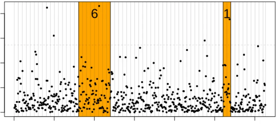
We report the results for chromosomec= 19, which containsmc= 626 genes.
In this particular case, we obtain trivial boundsζc,k(X) =|Rc,k|for allk∈NKc.
Therefore, the proxy ˜VR∗ defined in (13) for disjoint sets does not identify any signal for this chromosome. However, non-trivial bounds can be obtained via the multi-scale approach briefly mentioned in Section7. The idea is to enrich the reference family by recursive binary aggregation of the neighboring Rc,k.
The total number of elements in this family is less than 2Kc. In our example,
it turns out that (15) yields 6 true discoveries in the intervalR17:24 and 1 true discovery in the intervalR53:54, where we have denoted
Ru:v =
[
u≤k≤v
Rc,k.
This is illustrated by Figure7 where the individual p-values are displayed (on the −log10 scale) as a function of their order on chromosome 19. The sets
R17:24 and R53:54 are highlighted in orange, with the corresponding number
of true discoveries marked in each region. We obtain a non-trivial bound not
● ●●● ● ● ● ● ● ● ● ● ● ● ● ● ● ● ● ● ● ● ● ● ● ● ● ● ● ● ● ●● ● ● ● ● ● ● ● ● ●● ● ● ● ● ● ● ● ● ● ● ● ● ● ● ● ● ● ● ● ●● ● ● ● ●● ● ● ●●● ● ● ● ● ● ● ● ● ● ● ● ● ● ● ● ● ● ● ● ● ● ● ● ● ● ● ● ● ● ● ●● ● ●●● ● ● ● ● ● ●● ● ● ● ● ● ● ● ● ● ● ● ● ● ● ● ● ● ● ● ● ● ● ● ● ●● ● ● ● ● ● ● ● ● ● ● ● ● ● ● ●● ● ● ● ● ● ● ● ● ● ● ● ● ● ● ● ● ● ● ● ● ● ● ● ● ● ●● ● ● ● ● ● ● ● ● ● ● ● ● ● ● ● ●● ● ● ● ● ●● ● ● ● ● ● ● ● ● ● ● ● ● ● ●● ● ● ● ● ●● ● ● ● ● ● ● ● ● ●● ●● ● ●● ● ● ●● ● ● ● ● ● ● ● ● ● ● ● ● ●● ● ●● ● ● ● ● ● ● ● ● ● ● ● ● ● ● ● ● ● ● ● ● ● ●● ● ● ● ● ● ● ● ● ● ● ● ● ● ● ● ● ● ● ● ● ● ● ● ● ● ●● ● ● ● ● ● ● ● ● ● ● ● ●● ●● ● ● ● ● ● ● ● ● ● ● ● ● ● ● ● ● ● ● ● ● ● ● ● ● ● ● ● ● ● ● ● ● ● ● ● ● ● ● ● ● ● ● ● ● ● ● ● ● ● ● ● ● ● ● ● ● ● ● ● ● ● ● ● ● ● ● ● ● ● ● ● ● ● ● ● ● ● ● ● ● ● ● ● ● ● ● ● ● ● ● ● ● ● ● ● ● ● ● ● ● ●● ● ● ● ● ● ● ● ● ● ●● ● ● ●●● ● ● ● ● ● ● ● ● ●● ● ● ● ● ●● ● ●● ● ●● ● ● ● ● ● ● ● ● ● ● ● ● ● ● ● ● ●● ● ● ● ● ● ● ● ● ● ● ● ● ● ● ● ● ● ●● ● ● ● ●●● ● ● ● ●● ● ● ● ● ● ● ● ● ● ● ●● ● ●● ● ● ● ● ● ● ● ●● ● ●●●●●● ● ● ● ● ● ● ● ● ● ● ●● ●● ● ● ● ● ●● ● ● ● ● ● ● ● ● ● ● ● ● ● ● ● ● ● ● ● ●●● ●● ● ● ● ● ●● ● ● ● ● ● ● ● ● ● ● ● ● ● ● ● ●● ● ● ● ● ● ● ● ● ● 0 100 200 300 400 500 600 0 1 2 3 4
Gene order on chromosome 19
− lo g10 ( p )
1
6
● ●●● ● ● ● ● ● ● ● ● ● ● ● ● ● ● ● ● ● ● ● ● ● ● ● ● ● ● ● ●● ● ● ● ● ● ● ● ● ●● ● ● ● ● ● ● ● ● ● ● ● ● ● ● ● ● ● ● ● ●● ● ● ● ●● ● ● ●●● ● ● ● ● ● ● ● ● ● ● ● ● ● ● ● ● ● ● ● ● ● ● ● ● ● ● ● ● ● ● ●● ● ●●● ● ● ● ● ● ●● ● ● ● ● ● ● ● ● ● ● ● ● ● ● ● ● ● ● ● ● ● ● ● ● ●● ● ● ● ● ● ● ● ● ● ● ● ● ● ● ●● ● ● ● ● ● ● ● ● ● ● ● ● ● ● ● ● ● ● ● ● ● ● ● ● ● ●● ● ● ● ● ● ● ● ● ● ● ● ● ● ● ● ●● ● ● ● ● ●● ● ● ● ● ● ● ● ● ● ● ● ● ● ●● ● ● ● ● ●● ● ● ● ● ● ● ● ● ●● ●● ● ●● ● ● ●● ● ● ● ● ● ● ● ● ● ● ● ● ●● ● ●● ● ● ● ● ● ● ● ● ● ● ● ● ● ● ● ● ● ● ● ● ● ●● ● ● ● ● ● ● ● ● ● ● ● ● ● ● ● ● ● ● ● ● ● ● ● ● ● ●● ● ● ● ● ● ● ● ● ● ● ● ●● ●● ● ● ● ● ● ● ● ● ● ● ● ● ● ● ● ● ● ● ● ● ● ● ● ● ● ● ● ● ● ● ● ● ● ● ● ● ● ● ● ● ● ● ● ● ● ● ● ● ● ● ● ● ● ● ● ● ● ● ● ● ● ● ● ● ● ● ● ● ● ● ● ● ● ● ● ● ● ● ● ● ● ● ● ● ● ● ● ● ● ● ● ● ● ● ● ● ● ● ● ● ●● ● ● ● ● ● ● ● ● ● ●● ● ● ●●● ● ● ● ● ● ● ● ● ●● ● ● ● ● ●● ● ●● ● ●● ● ● ● ● ● ● ● ● ● ● ● ● ● ● ● ● ●● ● ● ● ● ● ● ● ● ● ● ● ● ● ● ● ● ● ●● ● ● ● ●●● ● ● ● ●● ● ● ● ● ● ● ● ● ● ● ●● ● ●● ● ● ● ● ● ● ● ●● ● ●●●●●● ● ● ● ● ● ● ● ● ● ● ●● ●● ● ● ● ● ●● ● ● ● ● ● ● ● ● ● ● ● ● ● ● ● ● ● ● ● ●●● ●● ● ● ● ● ●● ● ● ● ● ● ● ● ● ● ● ● ● ● ● ● ●● ● ● ● ● ● ● ● ● ●Fig 7. Evidence of locally-structured signal on chromosome 19 detected by the bound (15).
because of the large effect of any individual gene, but because of the presence of sufficiently many moderate effects. In particular, in the rightmost orange
region in Figure 7, the distribution of −log10(p) is shifted away from 0 when compared to the rest of chromosome 19. In comparison, we obtain trivial bounds
VR(R53:54) =|R53:54|= 2sand VR(R17:24) =|R17:24|= 8sfrom (12) both for
the linear or the beta template. These numerical results illustrate the interest of the bounds introduced in Section7in situations where one expects the signal to be spatially structured.
9. Bibliographical notes
The material exposed in this chapter is mainly a digested account of the ar-ticle [2]. The seminal work [9] introduced the idea of false positive bounds for arbitrary rejection sets. It started from the idea of building a confidence set on the set of null hypotheses H0(P), and introduced the concepts of augmenta-tion procedure and inversion procedure. The latter consists in building a con-fidence set based on the inversion of tests for H0(P) = A for all A ⊂ Nm.
The former starts from a set R with controlled k-familywise error rate, and the proposed associated post hoc bound is (10) (for the one-element reference family (R, ζ =k−1)). The name augmentation refers to a similar idea found in [6]. The relaxation (10) can in this sense be called “generalized augmentation procedure”. A post hoc bound for an arbitrary rejection set based on a closed test principle was proposed in [10]. It can also be seen as a reformulation of the inversion procedure of [9]. Post-hoc bounds over a large class of reference families extracted from classical FDR control procedures combined with mar-tingale techniques were recently proposed in [14]. The principle of the graphical representation used in Figure1 to visualize the Simes inequality-based bound originates from J. Goeman.
The use of generalized permutation procedures in a multiple testing frame-work has been explored in several landmark frame-works [22, 19, 17,6, 11, 13]. The subset-pivotality condition has been defined in [22]. Assumption (Rand) has been introduced in [12] and is a weaker version of the randomization hypothesis of [19]. The phenomenon of conservativeness in the permutation-based calibra-tion mencalibra-tioned at the end of Seccalibra-tion 4, when not all the null hypotheses are true, can be in part alleviated by using a step-down principle (see [19] for a sem-inal work on this topic and [2] for more details on this approach in the specific setting considered here). The choice of the sizeKof the reference family, which can be crucial in practice, is also discussed in [2].
Multiple testing for spatially structured hypotheses is in itself a very active and broad area of research. It has been specifically considered in conjunction with post-hoc bounds in [16]. The use of the reference family approach for post-hoc bounds in combination with spatially structured hypotheses has been studied in [7], where the notion of tree- (or forest-)structured reference regions is introduced, along with an efficient algorithm to compute the optimal bound V∗
R in this setting.
The Simes inequality [20] is a particularly nice and elegant theoretical device with manifold applications in multiple testing which is still a very active research
area, see, e.g., [3,4,8]. The DKW inequality with optimal constant was proved in [15]. The Benjamini-Hochberg (BH) procedure has been introduced in [1], where it is also proved to control the false discovery rate (FDR). A huge literature on FDR control has followed this seminal paper.
The data used for the application part are taken from [5]. The fact that the signal is clustered along the genome is motivated by previous studies showing possible links between gene expression and DNA copy number changes or other regulation mechanisms [18,21].
Acknowledgements
This work has been supported by 16-CE40-0019 (SansSouci) and ANR-17-CE40-0001 (BASICS). The first author acknowledges the support from the german DFG under the Collaborative Research Center SFB-1294 “Data Assim-ilation”.
References
[1] Y. Benjamini and Y. Hochberg. Controlling the false discovery rate: a practical and powerful approach to multiple testing. J. Roy. Statist. Soc. Ser. B, 57(1):289–300, 1995.
[2] G. Blanchard, P. Neuvial, and E. Roquain. Post hoc confidence bounds on false positives using reference families. Annals of Statistics, to appear. [3] H. W. Block, T. H. Savits, J. Wang, and S. K. Sarkar. The multivariate-t
distribution and the Simes inequality.Statist. Probab. Lett., 83(1):227–232, 2013.
[4] T. Bodnar and T. Dickhaus. On the Simes inequality in elliptical models.
Ann. Inst. Statist. Math., 69(1):215–230, 2017.
[5] S. Chiaretti, X. Li, R. Gentleman, A. Vitale, K. S. Wang, F. Mandelli, R. Foa, and J. Ritz. Gene expression profiles of b-lineage adult acute lymphocytic leukemia reveal genetic patterns that identify lineage deriva-tion and distinct mechanisms of transformaderiva-tion. Clinical cancer research, 11(20):7209–7219, 2005.
[6] S. Dudoit and M. J. van der Laan. Multiple testing procedures with ap-plications to genomics. Springer Series in Statistics. Springer, New York, 2008.
[7] G. Durand, G. Blanchard, P. Neuvial, and E. Roquain. Post hoc false posi-tive control for spatially structured hypotheses.arXiv preprint 1807.01470, Jul 2018.
[8] H. Finner, M. Roters, and K. Strassburger. On the Simes test under de-pendence. Statist. Papers, 58(3):775–789, 2017.
[9] C. R. Genovese and L. Wasserman. Exceedance control of the false discov-ery proportion. J. Amer. Statist. Assoc., 101(476):1408–1417, 2006. [10] J. J. Goeman and A. Solari. Multiple testing for exploratory research.
[11] J. Hemerik and J. Goeman. Exact testing with random permutations.
TEST, 27(4):811–825, 2018.
[12] J. Hemerik and J. J. Goeman. False discovery proportion estimation by permutations: confidence for significance analysis of microarrays. Journal of the Royal Statistical Society: Series B (Statistical Methodology), 2017. [13] J. Hemerik, A. Solari, and J. J. Goeman. Permutation-based simultaneous
confidence bounds for the false discovery proportion.Biometrika, to appear. [14] E. Katsevich and A. Ramdas. Simultaneous high-probability bounds on the false discovery proportion in structured, regression, and online settings, 2018. arXiv preprint 1803.06790.
[15] P. Massart. The tight constant in the Dvoretzky-Kiefer-Wolfowitz inequal-ity. Ann. Probab., 18(3):1269–1283, 1990.
[16] R. J. Meijer, T. J. Krebs, and J. J. Goeman. A region-based multiple testing method for hypotheses ordered in space or time. Statistical Applications in Genetics and Molecular Biology, 14(1):1–19, 2015.
[17] N. Meinshausen. False discovery control for multiple tests of association under general dependence. Scand. J. Statist., 33(2):227–237, 2006.
[18] F. Reyal, N. Stransky, I. Bernard-Pierrot, A. Vincent-Salomon, Y. de Rycke, P. Elvin, A. Cassidy, A. Graham, C. Spraggon, Y. D´esille, A. Fourquet, C. Nos, P. Pouillart, H. Magdel´enat, D. Stoppa-Lyonnet, J. Couturier, B. Sigal-Zafrani, B. Asselain, X. Sastre-Garau, O. Delattre, J. P. Thiery, and F. Radvanyi. Visualizing chromosomes as transcrip-tome correlation maps: evidence of chromosomal domains containing co-expressed genes - a study of 130 invasive ductal breast carcinomas. Cancer Research, 65(4):1376–1383, Feb. 2005.
[19] J. P. Romano and M. Wolf. Exact and approximate stepdown methods for multiple hypothesis testing. J. Amer. Statist. Assoc., 100(469):94–108, 2005.
[20] R. J. Simes. An improved Bonferroni procedure for multiple tests of sig-nificance. Biometrika, 73(3):751–754, 1986.
[21] N. Stransky, C. Vallot, F. Reyal, I. Bernard-Pierrot, S. G. D. de Med-ina, R. Segraves, Y. de Rycke, P. Elvin, A. Cassidy, C. Spraggon, A. Gra-ham, J. Southgate, B. Asselain, Y. Allory, C. C. Abbou, D. G. Albertson, J.-P. Thiery, D. K. Chopin, D. Pinkel, and F. Radvanyi. Regional copy number-independent deregulation of transcription in cancer. Nature Ge-netics, 38:1386–1396, 2006.
[22] P. H. Westfall and S. S. Young.Resampling-Based Multiple Testing. Wiley, 1993.