PLUG-IN BANDWIDTH SELECTOR FOR THE KERNEL RELATIVE
DENSITY ESTIMATOR
ELISA MAR´IA MOLANES-L ´OPEZ1 AND RICARDO CAO1
1Departamento de Matem´aticas, Facultade de Inform´atica, Universidade da Coru˜na,
Campus de Elvi˜na s/n, 15071 A Coru˜na, Spain
BANDWIDTH SELECTION FOR THE RELATIVE DENSITY
Abstract. This paper is focused on two kernel relative density estimators in a two-sample problem. An asymptotic expression for the mean integrated squared error of these estimators is found and, based on it, two solve-the-equation plug-in bandwidth selectors are proposed. In order to examine their practical perfor-mance a simulation study and a practical application to a medical dataset are carried out.
Key words and phrases: kernel-type estimates, smoothing parameter, solve-the-equation rules, survival analysis, two-sample problem.
1. Introduction
The study of differences among groups or changes over time is a goal in fields such as medical research and social science research. The traditional method for this purpose is the usual parametric location and scale analysis. However, this is a very restrictive tool, since a lot of the information available in the data is unaccessible. In order to make a better use of this information it is convenient to focus on distributional analysis, i.e.,
on the general two-sample problem of comparing the cumulative distribution functions (cdf), F0 and F, of two random variables, X0 and X. Useful tools for this purpose are
the relative distribution function,R(t), and the relative density function,r(t), ofX with respect to (w.r.t.) X0:
R(t) =P (F0(X)≤t) = F F0−1(t)
, 0< t <1
where F0−1(t) = inf{x|F0(x)≥t} denotes the quantile function of F0 and
r(t) = R(1)(t) = f F −1 0 (t) f0 F0−1(t) , 0< t <1
wheref andf0are the densities pertaining toF andF0, respectively. These two curves, as
well as estimators for them, have been studied by Gastwirth (1968), ´Cwik and Mielniczuk (1993), Hsieh (1995), Hsieh and Turnbull (1996), Cao et al. (2000, 2001) and Handcock and Janssen (2002).
These functions, R and r, are closely related to other statistical methods. The ROC curve, used in the evaluation of the performance of medical tests for separat-ing two groups, is related to R through the relationship ROC(t) = 1−R(1−t) (see, for instance, Holmgren (1996) and Li et al. (1996) for details) and the density ratio
h(x) = ff(x)0(x), x∈R, used by Silverman (1978) is linked to r throughh(x) = r(F0(x)).
Throughout the paper, we will focus on two kernel-type estimators of r, similar to the one already proposed by ´Cwik and Mielniczuk (1993). In the following section we will give some notation and obtain an asymptotic representation for the MISE of the relative density estimators. This is a difference with respect to ´Cwik and Mielniczuk (1993), where an asymptotic expression for the MISE of only the dominant part of the estimator was found. Section 3 is concerned with automatic global bandwidth selection. Two solve-the-equation plug-in bandwidth selectors based on the ideas by Sheather and Jones
(1991) are proposed. A simulation study is shown in Section 4 where the performance of the data-driven selectors proposed in this paper is compared with the selector proposed in ´Cwik and Mielniczuk (1993). A medical application is presented in Section 5. Finally, the proofs of the results presented in Sections 2 and 3 are included in Section 6.
2. Kernel relative density estimators
Consider the two-sample problem with completely observed data:
{X01, . . . , X0n}, {X1, . . . , Xm}
where the X0i’s are independent and identically distributed as X0; and the Xj’s are
independent and identically distributed asX. These two sequences are independent each other.
Throughout this paper all the asymptotic results are obtained if both sample sizesm
and n tend to infinity in such a way that, for some constant 0< λ <∞,
lim
m−→∞
m n =λ.
We assume the following conditions on the underlying distributions, the kernels K
and M and the bandwidths h and h0 to be used in the estimators (see (1), (2) and (3)
below):
(F1) F0 and F have continuous density functions, f0 and f, respectively.
(F2) f0 is a three times differentiable density function withf0(3) bounded.
(R1) r is a differentiable density with compact support contained in [0,1] with r(1)
(K1) K is a symmetric four times differentiable density function with compact support [−1,1] andK(4) bounded.
(K2) M is a symmetric density and continuous function except at a finite set of points.
(B1) h−→0 andmh3 −→ ∞. (B2) h0 −→0 andnh40 −→0. Since 1 h R1 0 K t−z h
dR(z) is close to r(t) and for smooth distributions it is satisfied that: 1 h Z 1 0 K t−z h dR(z) = 1 h Z ∞ −∞ K t−F0(z) h dF(z),
a natural way to define a kernel-type estimator ofr(t) is to replace the unknown functions
F0 and F by some appropriate estimators. We consider two proposals:
(1) rˆh(t) = Z ∞ −∞ Kh(t−F0n(z))dFm(z) = 1 m m X j=1 Kh(t−F0n(Xj)) and (2) rˆh,h0(t) = Z ∞ −∞ Kh t−F˜0n(z) dFm(z) = 1 m m X j=1 Kh t−F˜0n(Xj) , where Kh(t) = 1hK ht
, K is a kernel function, h is the bandwidth used to estimate r,
F0nandFm are the empirical distribution functions based onX0i’s andXj’s, respectively,
and ˜F0n is a kernel-type estimate of F0 given by:
(3) F˜0n =n−1 n X i=1 M x−X0i h0
Using a Taylor expansion, ˆrh(t) can be written as follows: ˆ rh(t) = Z ∞ −∞ Kh(t−F0(z))dFm(z) + Z ∞ −∞ Kh(1)(t−F0(z)) (F0(z)−F0n(z))dFm(z) + Z ∞ −∞ (F0(z)−F0n(z))2 Z 1 0 (1−s)Kh(2)(t−F0(z)−s(F0n(z)−F0(z)))dsdFm(z).
Let us define ˜Un=F0n◦F0−1 and ˜Rm =Fm◦F0−1. Then, ˆrh(t) can be rewritten in a
useful way for the study of its mean integrated squared error (MISE):
(4) rˆh(t) = ˜rh(t) +A1+A2+B,where ˜ rh(t) = Z ∞ −∞ Kh(t−F0(z))dFm(z) = 1 m m X j=1 Kh(t−F0(Xj)) A1 = Z 1 0 v−U˜n(v) Kh(1)(t−v)dR˜m−R (v) A2 = 1 n n X i=1 Z ∞ −∞ (F0(w)−1{X0i ≤w})Kh(1)(t−F0(w))dF(w) B = Z ∞ −∞ (F0(z)−F0n(z))2 Z 1 0 (1−s)Kh(2)(t−F0(z)−s(F0n(z)−F0(z)))dsdFm(z).
Proceeding in a similar way, we can rewrite ˆrh,h0 as follows:
(5) rˆh,h0(t) = ˜rh(t) +A1+A2 + ˆA+ ˆB,where ˆ A = Z F0n(w)−F˜0n(w) Kh(1)(t−F0(w))dFm(w) ˆ B = Z ∞ −∞ (F0(z)−F˜0n(z)) 2Z 1 0 (1−s)Kh(2)t−F0(z)−s ˜ F0n(z)−F0(z) dsdFm(z).
Our main result is an asymptotic representation for the MISE of ˆrh(t) and ˆrh,h0(t).
With the purpose of simplifying the exposition of the results obtained, from here on we will denote C(g) = R∞
−∞g
Theorem 1 (AMISE). Assume conditions (F1), (R1), (K1) and (B1). Then M ISE(ˆrh) = AM ISE(h) +o 1 mh +h 4 +o 1 nh AM ISE(h) = 1 mhC(K) + 1 4h 4d2 KC(r(2)) + 1 nhC(r)C(K) where dK = R1 −1x 2K(x)dx.
If the conditions (F2), (K2), and (B2) are assumed as well, then the same result is satisfied for the M ISE(ˆrh,h0).
Remark 1. From Theorem 1 it follows that the optimal bandwidth, minimizing the asymptotic mean integrated squared error of any of the estimators considered for r, is given by (6) hAM ISE = C(K)(λC(r) + 1) d2 KC(r(2))m 15 .
Remark 2. Note that AM ISE(h) derived from Theorem 1 does not depend on the bandwidth h0. A more higher-order analysis should be considered to address
simultane-ously the bandwidth selection problem of h and h0.
3. Bandwidth selectors
3.1 Estimation of density functionals
It is very simple to show that, under sufficiently smooth conditions on r (r ∈
C(2`)(R)), the functionals (7) C r(`) = Z 1 0 r(`)(x)2dx
appearing in (6), are related to other general functionals of r, denoted by Ψ2`:
(8) C r(`)
= (−1)`
Z 1 0
where Ψ` = Z 1 0 r(`)(x)r(x)dx=E r(`)(F0(X)) .
The equation above suggests a natural kernel-type estimator for Ψ` as follows
(9) Ψˆ`(g) = 1 m m X j=1 " m X k=1 1 mL (`) g (F0n(Xj)−F0n(Xk)) #
where L is a kernel function and g is a smoothing parameter called pilot bandwidth. Likewise in the previous section, this is not the unique possibility and we could consider another estimator of Ψ`, (10) Ψ˜`(g) = 1 m m X j=1 " m X k=1 1 mL (`) g ˜ F0n(Xj)−F˜0n(Xk) # ,
where F0n in (9) is replaced by ˜F0n. Since the difference between both estimators
de-creases as h0 tends to zero, it is expected to obtain the same theoretical results for both
estimators. Therefore, we will only show theoretical results for ˆΨ`(g).
We will obtain the asymptotic mean squared error of ˆΨ`(g) under the following
as-sumptions.
(R3) The relative density r ∈C(`+6)(R).
(K3) The kernel L is a symmetric kernel of order 2, L ∈ C(`+7)(R) and satisfies that
(−1)`2+2L(`)(0)d
L>0, L(`)(1) =L(`+1)(1) = 0, with dL= R∞
−∞x2L(x)dx. (B3) g =gm is a positive-valued sequence of bandwidths satisfying
lim m−→∞g = 0 and m−→∞lim mg max{α,β} =∞ where α= 2 (`+ 7) 5 , β = 1 2(`+ 1) + 2.
Condition (R3) implies a smooth behaviour of r in the boundary of its support, contained in [0,1]. If this smoothness fails, the quantity C r(`)
could be still estimated through its definition, using a kernel estimation for r(`) (see Hall and Marron (1987) for
the one-sample problem setting). Condition (K3) can only hold for even `. Observe that in condition (B3) for even `, max{α, β} = α for ` = 0,2 and max{α, β} = β for
`= 4,6, . . .
Theorem 2. Assume conditions (F1), (R3), (K3) and (B3). Then it follows that
M SEΨˆ`(g) = 1 mg`+1L (`)(0) (1 +λΨ 0) + 1 2dLΨ`+2g 2+O g4 (11) +o ng`+1−1i2+ 2 m2g2`+1Ψ0C L (`) +o m2g2`+1−1+O n−1 .
Remark 3. The first term in the right-hand side of (11) corresponds to the squared bias term of MSE. Note that, using (K3) and (8), the main bias term can be made to vanish by choosing g asg` g` = 2L(`)(0) (λΨ 0 + 1) −dLΨ`+2m (`+3)1 = 2L`(0)d2 KΨ4 −dLΨ`+2C(K) `+31 h 5 `+3 AM ISE.
3.2 STE rules based on Sheather & Jones ideas
As in the context of ordinary density estimation, the practical implementation of the kernel-type estimators proposed here (see (1) and (2)), requires the choice of the smoothing parameter h. Our two proposals, hSJ1 and hSJ2, as well as the selector b3c
recommended by ´Cwik and Mielniczuk (1993), are modifications of Sheather & Jones (1991). Since the Sheather & Jones selector is the solution of an equation in the band-width, it is also known as a solve-the-equation (STE) rule. Motivated by the formula (6)
for the AMISE-optimal bandwidth and the relation (8), solve-the-equation rules require that h is chosen to satisfy the relationship
h= C(K)λΨ˜0(γ1(h)) + 1 d2 K·Ψ˜4(γ2(h))·m 1 5 ,
where the pilot bandwidths for the estimation of Ψ0 and Ψ4 are functions ofh(γ1(h) and
γ2(h), respectively).
Motivated by Remark 3, we suggest taking
γ1(h) = 2·L(0)·d2 K ·Ψ˜4(g4) −dLΨ˜2(g2)C(K) !13 h53 and γ2(h) = 2·L(4)(0)·d2 K·Ψ˜4(g4) −dLΨ˜6(g6)C(K) !17 h57,
where ˜Ψj(·), (j = 0,2,4,6) are kernel estimates (10). Note that this way of proceeding
leads us to a never ending process in which a bandwidth selection problem must be solved at every stage. To make this iterative process feasible in practice one possibility is to propose a stopping stage in which the unknown quantities are estimated using a parametric scale for r. This strategy is known in the literature as the stage selection problem (see Wand and Jones (1995)). While the selector b3c in ´Cwik and Mielniczuk
(1993) used a Gaussian scale, now for the implementation of hSJ2, we will use a mixture
of betas based on the Weierstrass approximation theorem and Bernstein polynomials associated to any continuous function on [0,1] (see Kakizawa (2004) and references therein for the motivation of this method). Later on we will show the formula for computing the reference scale above-mentioned, together with the selector b3c we used in Section 4.
In the following we denote the Epanechnikov kernel by K, the uniform density in [−1,1] by M and we define L as follows
L(x) = Γ(18) 2Γ(9)Γ(9) x+ 1 2 8 1− x+ 1 2 8 1{−1≤x≤1}.
Next, we detail the steps required in the implementation ofhSJ2.
Step 1. Obtain ˆΨP R
j (j = 0,4,6,8), parametric estimates for Ψj(j = 0,4,6,8), with the
replacement of r in C r(j/2)
(see (7)), by a mixture of betas, b(x), as it will be explained later on (see (12)).
Step 2. Compute kernel estimates for Ψj(j = 2,4,6), by using ˜Ψj(gjP R)(j = 2,4,6), with
gP Rj = 2·L(j)(0)λΨˆP R0 + 1 −dL·ΨˆP Rj+2·m 1 j+3 ,(j = 2,4,6).
Step 3. Estimate Ψ0 and Ψ4, using (10), by means of ˜Ψ0(ˆγ1(h)) and ˜Ψ4(ˆγ2(h)), where
ˆ γ1(h) = 2·L(0)·d2 K·Ψ˜4 gP R4 −dLΨ˜2(gP R2 )C(K) !13 h53 and ˆ γ2(h) = 2·L(4)(0)·d2 K·Ψ˜4 gP R4 −dLΨ˜6(g6P R)C(K) !17 h57.
Step 4. Select the bandwidth hSJ2 as the one that solves the following equation inh:
h = C(K)λΨ˜0(ˆγ1(h)) + 1 d2 K ·Ψ˜4(ˆγ2(h))·m 1 5 .
In order to solve the equation above, it will be necessary to use a numerical algorithm. In the simulation study we will use the false-position method. The main reason is that the false-position algorithm does not require the computation of the derivatives, what simplifies considerably the implementation of the proposed bandwidth selectors. At the same time, this algorithm presents some advantages over others because it tries to com-bine the speed of methods such as the secant method with the security afforded by the bisection method.
Unlike the Gaussian parametric reference, used to obtain b3c, the selector hSJ2 uses
in Step 1 a mixture of betas as follows:
(12) b(x) = N X j=1 ˜ Rn,m j N −R˜n,m j −1 N β(x, j, N −j+ 1) where ˜ Rn,m(x) = m−1 m X j=1 M x−F˜0n(Xj) g ! , (13) g = 2 R∞ −∞xM(x)M(x)dx nd2 MC(r(1)) !13 , (14)
β(x, a, b) stands for the beta density
β(x, a, b) = Γ(a+b) Γ(a)Γ(b)x
a−1(1−x)b−1, x∈[0,1],
and N is the number of betas in the mixture.
Since we are trying to estimate a density with support in [0,1] it seems more suitable to consider a parametric reference with this support. A mixture of betas is an appropriate option because it is flexible enough to model a large variety of relative densities, when derivatives of order 1, 3 and 4 are also required.
Note that, for the sake of simplicity, we are using above the AMISE-optimal band-width (g) for estimating a distribution function in the setting of a one-sample problem (see Polansky and Baker (2000) for more details in the kernel-type estimate of a distribution function). The use of this bandwidth requires the previous estimation of the unknown functional, C r(1)
. We will consider a quick and dirty method, the rule of thumb, that uses a parametric reference for r to estimate the above-mentioned unknown quantity. More specifically, our reference scale will be a beta with parameters (p, q) estimated from the smoothed relative sample nF˜0n(Xj)
om
j=1, using the method of moments.
kernel-type estimator ˜F0n introduced in (3) is based on the AMISE-optimal bandwidth
in the one-sample problem:
h0 = 2R∞ −∞xM(x)M(x)dx nd2 MC f0(1) 1 3 .
As it was already mentioned above, in most of the cases this methodology will be applied to survival analysis, so it is natural to assume that our samples come from distribu-tions with support on the positive real line. Therefore, a gamma reference distribution, Gamma(α, β), has been considered, where the parameters (α, β) are estimated from the smoothed relative sample nF˜0n(Xj)
om
j=1, using the method of moments.
For the implementation of hSJ1, we proceed analogously to that of hSJ2 above. The
only difference now is that throughout the previous discussion, ˜Ψj(·) and ˜F0n(·) are
replaced by, respectively, ˆΨj(·) and F0n(·).
As a variant of the selector that ´Cwik and Mielniczuk (1993) proposed,b3cis obtained
as the soluction to the following equation:
b3c = C(K)1 +λΨˆ0(a) d2 KΨˆ4(α2(b3c))m 1 5 , where a = 1.781ˆσm−13, ˆσ = min n sm,IQR/[ 1.349 o
, sm and IQR[ denote, respectively,
the empirical standard deviation and the sample interquartile range of the relative data,
{F0n(Xj)}mj=1, α2(b3c) = 0.7694 ˆ Ψ4 gGS4 −Ψˆ6(gGS6 ) !17 b57 3c,
where GS stands for standard Gaussian scale,
g4GS= 1.2407ˆσm−
1
7, g6GS= 1.2304ˆσm− 1 9
and the estimates ˆΨj (with j = 0,4,6) were obtained using (9), with L replaced by
reducing the two-sample problem to a one-sample problem.
It is interesting to note that all the kernel-type estimators presented previously (ˆrh(t),
ˆ
rh,h0(t), ˜Rn,m(x) and ˜F0n(x)) were not corrected to take into account, respectively, the
fact that r and R have support on [0,1] instead of on the whole real line, and the fact that f0 is supported only on the positive real line. Therefore, in order to correct the
boundary effect in practical applications we will use the well known reflecting method to modify ˆrh(t), ˆrh,h0(t), ˜Rn,m(x) and ˜F0n(x), where needed.
4. Simulations
We compare, through a simulation study, the performance of the bandwidth selectors
hSJ1 and hSJ2, proposed in Section 3, with the standard competitor b3c recommended
by ´Cwik and Mielniczuk (1993). Although we are aware that the smoothing parameter
N introduced in (12) should be selected by some optimal way based on the data, this issue goes beyond the scope of this article. Consequently, from here on, we will consider
N = 14 components in the beta mixture reference scale model given by (12).
We will consider the first sample coming from the random variate X0 = W−1(U)
and the second sample coming from the random variateX1 =W−1(S), whereU denotes
a uniform distribution in the compact interval [0,1], W is the distribution function of a Weibull distribution with parameters (2,3) and S is a random variate from one of the following five different populations (see Figure 1):
(a) A beta distribution with parameters 14 and 17 (β(14,17)).
(b) A mixture consisting of V1 with probability 45 and V2 with probability 15, where
(c) A mixture consisting of V1 with probability 13 and V2 with probability 23, where
V1 =β(34,15) and V2 =β(15,30).
Put Figure 1 about here.
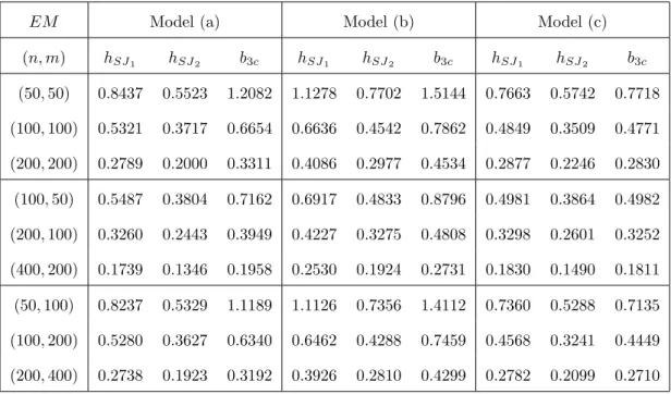
Choosing different values for the pair of sample sizesm and n and under each of the models presented above, we start drawing 500 pair of random samples and, according to every method, we select the bandwidths ˆh. Then, in order to check their performance we approximate by Monte Carlo the mean integrated squared error, EM, between the true relative density and the kernel-type estimate for r, given by (1) when ˆh=b3c, hSJ1 or by
(2) when ˆh=hSJ2.
The computation of the kernel-type estimations can be very time consuming by using a direct algorithm. Therefore, we will use linear binned approximations that, thanks to their discrete convolution structures, can be fast computed by using the fast Fourier transform (FFT) (see Wand and Jones (1995) for more details).
For all the models, the values of this criterion for the three bandwidth selectors,hSJ1,
hSJ2 and b3c, can be found in Table 1.
Put Table 1 about here.
A careful look at the table points out that the new selector hSJ2 presents a much
better behaviour than the selectorb3c, especially when the sample sizes are equal or when
mis larger thann. The improvement is even larger for unimodal relative densities (model (a) and (b)). On the other hand, it is observed that the other proposal, hSJ1, presents
only a moderate improvement overb3c for unimodal relative densities (model (a) and (b))
and performs only slightly better or even worse than b3c for bimodal relative densities
three selectors considered. For instance, it is clearly seen an asymmetric behaviour of the selectors in terms of the sample sizes.
Other proposals for selecting h have been investigated. For instance, versions of
hSJ2 were considered in which either the unknown functionals Ψ are estimated from the
viewpoint of a one-sample problem or the STE rule is modified in such a way that only the function ˆγ2 is considered in the equation to be solved (see Step 4 in Section 3).
After a simulation study similar to the one detailed here, but now carried out for these versions ofhSJ2, it was observed a similar practical performance to that observed forhSJ2.
However, a worse behaviour was observed when, in the implementation of these versions of hSJ2, the smooth estimate of F0 is replaced by the empirical distribution function
F0n. Therefore, although hSJ2 requires the selection of two bandwidth parameters, a
clear better practical behaviour is observed when considering the smoothed relative data instead of the non-smoothed ones.
5. A medical application
In this section we apply the plug-in STE selector hSJ2 detailed above, to estimate
the relative density for a real data set concerned with prostate cancer (PC).
The data consist of 599 patients suffering from PC (+) and 835 patients PC-free (-). For each patient the illness status has been determined through a prostate biopsy carried out for first time in Hospital Juan Canalejo (Galicia, Spain) between January of 2002 and September of 2005.
In the literature, there exists an increasingly interest in finding a good diagnostic test that helps in the early detection of PC and avoids the need of undergoing a prostate biopsy. There are several studies in which, through ROC curves, it was investigated the
performance of different diagnostic tests based on some analytic measurements such as the total prostate specific antigen (tPSA), the free PSA (fPSA) or the complexed PSA (cPSA).
As it was mentioned in Section 1, there exists a close relation between the concepts of ROC curve and relative density. Relative density estimates can provide more detailed information about the performance of a diagnostic test which can be useful not only in comparing different tests but also in designing an improved one. This issue goes beyond the scope of this article and therefore it will not be investigated here.
In this section we compare from a distributional point of view the above mentioned measurements (tPSA, fPSA and cPSA) among the two groups in the data set (PC+ and PC-). To this end we start computing the appropriate bandwidths using the data-driven bandwidth selectorhSJ2 and then the corresponding relative density estimates are
computed using (2). These estimates are shown in Figure 2.
Put Figure 2 about here.
It is clear from Figure 2 that the relative density estimate is above one in a central interval accounting for a probability of about 40% of the PC- distribution for the variables tPSA and cPSA. This is also the case in the 10% right tail of the PC- group for tPSA and cPSA, but not for fPSA. In the case of fPSA the central interval with relative density above one is slightly shifted to the left of the PC- distribution: between percentiles 20% and 60%.
6. Proofs
The proof of Theorem 1 will be a direct consequence of some previous lemmas where each one of the terms that result from expanding the expression for the MISE are studied.
Some of them will produce dominant parts in the final expression for the MISE while others will yield negligible terms.
Lemma 1. Assume the hypothesis above. Then
(i) R1 0 E[(˜rh(t)−r(t)) 2]dt= 1 mhC(K) R1 0 r(t)dt+ 1 4h 4d2 KC(r(2)) +o mh1 +h 4 . (ii) R1 0 E[A 2 2]dt = nh1 C(r)C(K) +o 1 nh =O nh1 . (iii) R1 0 E[A21]dt=o nh1 . (iv) R1 0 E[B 2]dt =o 1 nh . (v) R1 0 E[2A1(˜rh−r)(t)]dt= 0. (vi) R1 0 E[2A2(˜rh−r)(t)]dt= 0. (vii) R1 0 E[2B(˜rh−r)(t)]dt =o 1 mh+h 4 . (viii) R1 0 E[2A1A2]dt=o 1 mh+h 4 . (ix) R1 0 E[2A1B]dt =o 1 mh+h4 . (x) R1 0 E[2A2B]dt=o 1 nh +h4 .
Lemma 2. Assume the hypothesis above. Then
(i) R1 0 E[ ˆA 2]dt =o 1 nh . (ii) R1 0 E[ ˆB 2]dt=o 1 nh .
Proof of Lemma 1. The proof of (i) is not included here because it is a classical result in the setting of ordinary density estimation in a one-sample problem (see Wand and Jones (1995) for details).
We next prove (ii). Standard algebra gives
E[A22] = 1 n2h4 n X i=1 n X j=1 Z ∞ −∞ Z ∞ −∞ E (F0(w1)−1{X0i≤w1})(F0(w2)−1{X0j≤w2}) K(1) t−F0(w1) h K(1) t−F0(w2) h dF(w1)dF(w2).
Due to the independence between X0i and X0j for i6=j, and using the fact that
Cov(1{F0(X0i)≤u1},1{F0(X0i)≤u2}) = (1−u1)(1−u2)g0(u1∧u2),
where g0(t) = 1−tt , the previous expression can be rewritten as follows
E[A2 2] = 2 nh4 Z 1 0 Z 1 u2 (1−u1)(1−u2)g0(u2)K(1) t−u1 h K(1) t−u2 h r(u1)r(u2)du1du2 = − 1 nh4 Z 1 0 g0(u2)d Z 1 u2 (1−u1)K(1) t−u1 h r(u1)du1 2 .
Now, using integration by parts, it follows that
E[A22] =−1 nh4 ulim 2→1− g0(u2)G(u2)2+ 1 nh4 ulim 2→0+ g0(u2)G(u2)2 (15) + 1 nh4 Z 1 0 G(u2)2g0(1)(u2)du2 where G(u2) = Z 1 u2 (1−u1)K(1) t−u1 h r(u1)du1.
Since G is a bounded function and g0(0) = 0, the second term in the right hand side
of (15) vanishes to zero. On the other hand, due to the boundedness of K(1) and r, it
follows that|G(u2)| ≤ K(1) ∞krk∞ (1−u2)2
2 , which let us conclude that the first term in
(15) is zero as well. Therefore,
E[A22] = 1 nh4 Z 1 0 G(u2)2g0(1)(u2)du2. (16)
Now, using integration by parts, it follows that
G(u2) = −(1−u1)r(u1)hK t−u1 h 1 u2 + Z 1 u2 hK t−u1 h [−r(u1) + (1−u1)r(1)(u1)]du1 =h(1−u2)r(u2)K t−u2 h + h Z 1 u2 K t−u1 h [(1−u1)r(1)(u1)−r(u1)]du1,
and plugging this last expression in (16), it is concluded that E[A22] = 1 nh2(I21+ 2I22+I23), where I21= Z 1 0 r2(u2)K2 t−u2 h du2 I22 = Z 1 0 1 (1−u2) r(u2)K t−u2 h Z 1 u2 K t−u1 h [(1−u1)r(1)(u1)−r(u1)]du1du2 I23 = Z 1 0 1 (1−u2)2 Z 1 u2 Z 1 u2 K t−u1 h [(1−u1)r(1)(u1)−r(u1)] K t−u∗ 1 h [(1−u∗1)r(1)(u∗1)−r(u∗1)]du1du∗1du2. Therefore, (17) Z 1 0 E[A22]dt= Z 1 0 1 nh2I21dt+ 2 Z 1 0 1 nh2I22dt+ Z 1 0 1 nh2I23dt.
Next, we will study each summand in (17) separately. The first term can be handled by using changes of variable and a Taylor expansion:
Z 1 0 1 nh2I21 dt = 1 nh Z 1 0 r2(u 2) Z 1−hu2 −u2 h K2(s)ds ! du2. Let us define K2(x) = Rx −∞K
2(s)ds and rewrite the previous term as follows Z 1 0 1 nh2I21 dt = 1 nh Z 1 0 r2(u2) K2 1−u2 h −K2 −u2 h du2.
Now, by splitting the integration interval into three subintervals: [0, h], [h,1−h] and [1−h,1], using changes of variable and the fact that
K2(x) = C(K) ∀x≥1 0 ∀x≤ −1,
it is easy to show that Z 1 0 1 nh2I21 dt= 1 nhC(K)·C(r) +O 1 n .
Below, we will study the second term in the right hand side of (17). By using changes of variable, Cauchy-Schwarz inequality and conditions krk∞< ∞, r(1)
∞< ∞
and C(K)<∞, straightforward calculations lead to
Z 1 0 1 nh2I22 dt=O 1 n + 1 nh12 =O 1 nh12 .
Similar arguments give
Z 1 0 1 nh2I23 dt=O 1 nh12 .
Therefore, it has been shown that
Z 1 0 E[A22]dt= 1 nhC(r)C(K) +O 1 n +O 1 nh12
Finally the proof of (ii) concludes using condition (B1). We now prove (iii). Direct calculations lead to
(18) E[A21] = 1 h4E[I1] where I1 =E Z 1 0 Z 1 0 (v1−U˜n(v1))(v2 −U˜n(v2))K(1) t−v1 h K(1) t−v2 h (19) d( ˜Rm−R)(v1)d( ˜Rm−R)(v2)/X01, . . . , X0n i .
To tackle with (18) we first study the conditional expectation (19). It is easy to see that
I1 =V ar[V /X01, . . . , X0n] where V = 1 m m X j=1 Xj−U˜n(Xj) K(1) t−Xj h .
Thus I1 = 1 m ( Z 1 0 (v−U˜n(v))K(1) t−v h 2 dR(v)− Z 1 0 (v−U˜n(v))K(1) t−v h dR(v) 2) and E[A21] = 1 mh4 Z 1 0 E h (v−U˜n(v)) i2 K(1) t−v h 2 dR(v)− 1 mh4 Z 1 0 Z 1 0 Eh(v1−U˜n(v1))(v2−U˜n(v2)) i K(1) t−v1 h K(1) t−v2 h dR(v1)dR(v2).
Taking into account that
E sup v |( ˜Un(v)−v)| 2 = Z ∞ 0 P sup v |( ˜Un(v)−v)| 2 > c dc,
we can use the Dvoretzky-Kiefer-Wolfowitz inequality, to conclude that
(20) E sup v |( ˜Un(v)−v)| 2 ≤ Z ∞ 0 2e−(2nc)dc= 2 n Z ∞ 0 ye−y2dy=O 1 n .
Consequently, using (20) and the conditions krk∞ < ∞ and K(1) ∞ < ∞ we obtain that E[A2 1] =O mnh1 4
. The proof of (iii) is concluded using condition (B1).
The results appearing in items (iv)-(x) can be proved by first conditioning to some appropriate random variables and then handling the conditional moments using standard arguments. For this reason their proofs are not included here.
Proof of Lemma 2. We start proving (i). Let us defineDn(w) = ˜F0n(w)−F0n(w), then E[ ˆA2] =E[E[ ˆA2/X1, . . . , Xm]] =E Z Z E[Dn(w1)Dn(w2)]Kh(1)(t−F0(w1))Kh(1)(t−F0(w2))dFm(v1)dFm(v2) .
Based on the results set for Dn(w) in Hjort and Walker (2001), the conditions (F2)
and (K2) and since E[Dn(w1)Dn(w2)] = Cov(Dn(w1), Dn(w2)) +E[Dn(w1)]E[Dn(w2)],
it follows that E[Dn(w1)Dn(w2)] =O h4 0 n +O(h4 0).
Therefore, for any t∈[0,1], we can boundE[ ˆA2], using suitable constantsC 2 andC3 as follows E[ ˆA2] =C2 h4 0 h4 1 m Z K(1) t−F0(z) h 2 f(z)dz +C3 h4 0 h4 (m−1) m Z Z K (1) t−F0(z1) h K (1) t−F0(z2) h f(z1)f(z2)dz1dz2.
Besides, the condition (R1) allows us to conclude that R
K(1)t−F0(z) h 2 f(z)dz = O(h) and RR K (1)t−F0(z1) h K (1)t−F0(z2) h f(z1)f(z2)dz1dz2 =O(h 2) for all t ∈[0,1]. Therefore,R1 0 E h ˆ A2idt =O h40 nh3 +Oh40 h2
, which, taking into account conditions (B1) and (B2), implies (i).
We next prove (ii). The proof is parallel to that of item (iv) in Lemma 1. The only difference now is that instead of requiringE[sup|F0n(x)−F0(x)|p] =O(n−
p
2), where pis
an integer larger than 1, it is required that
(21) Ehsup F˜0n(x)−F0(x) pi =O(n−p2).
To conclude the proof, below we show that (21) is satisfied. DefineHn= sup F˜0n(x)
−F0(x)|, then, as it is stated in Ahmad (2002), it follows thatHn ≤En+WnwhereEn=
sup|F0n(x)−F0(x)| and Wn = sup EF˜0n(x)−F0(x) = O(h 2
0). Using the binomial
formula it is easy to obtain that, for any integer p ≥ 1, Hp n ≤
Pp j=0C
p
jWnp−jEnj, where
the constantsCjp’s (withj ∈ {0,1, . . . , p−1, p}) are the binomial coefficients. Therefore, since E[Ej n] = O(n− j 2) and Wp−j n = O(h 2(p−j) 0 ), condition (B2) leads to Wnp−jE[Enj] = O(n−p2).
As a straightforward consequence, (21) holds and the proof of (ii) is concluded.
Proof of theorem 2. Below, we will briefly detail the steps followed to study the asymptotic behaviour of the mean squared error of ˆΨ`(g) defined in (9). First of all, let
us observe that ˆ Ψ`(g) = 1 mL (`) g (0) + 1 m2 m X j=1 m X k=1,j6=k L(`)g (F0n(Xj)−F0n(Xk)), which implies: EhΨˆ`(g) i = 1 mg`+1L (`)(0) + 1− 1 m E L(`)g (F0n(X1)−F0n(X2)) .
Starting from the equation
E L(`) g (F0n(X1)−F0n(X2)) = E E L(`)g (F0n(X1)−F0n(X2))/X01, ..., X0n = E Z ∞ −∞ Z ∞ −∞ L(`)g (F0n(x1)−F0n(x2))f(x1)f(x2)dx1dx2 = Z ∞ −∞ Z ∞ −∞ E L(`)g (F0n(x1)−F0n(x2)) f(x1)f(x2)dx1dx2
and using a Taylor expansion, we have
(22) E L(`)g (F0n(X1)−F0n(X2)) = 7 X i=0 Ii where I0 = Z ∞ −∞ Z ∞ −∞ 1 g`+1L (`) F0(x1)−F0(x2) g f(x1)f(x2)dx1dx2 Ii = Z ∞ −∞ Z ∞ −∞ 1 i!g`+i+1L (`+i) F0(x1)−F0(x2) g Eh(F0n(x1)−F0(x1)−F0n(x2) +F0(x2))i i f(x1)f(x2)dx1dx2 i= 1, . . . ,6 I7 = Z ∞ −∞ Z ∞ −∞ 1 7!g`+7+1E L(`+7)(ξn) (F0n(x1)−F0(x1)−F0n(x2) +F0(x2))7 f(x1)f(x2)dx1dx2
Now, consider the first term,I0, in (22). It is easy to see that I0 = Z 1 0 Z 1 0 L(`)g (z1−z2)r(z1)r(z2)dz1dz2 = Z 1 0 Z 1 0 Lg(x)r(z1−z2)r(`)(z2)dz1dz2 = Z 1 0 Z (1−z2)/g 0 L(x)r(z2+gx)r(`)(z2)dxdz2,
hence using a Taylor expansion, we have I0 = Ψ` + (1/2)dLΨ`+2g2 +O(g4). Assume
x1 > x2 and define Z =Pni=11{x2<X0i≤x1}. Then, the random variable Z has a Bi(n, p)
distribution with p = F0(x1)−F0(x2) and mean µ = np. It is easy to show that, for
i= 1, . . . ,6, Ii = 2 Z ∞ −∞ Z ∞ x2 1 i!g`+i+1L (`+i) F0(x1)−F0(x2) g f(x1)f(x2) 1 niµi(Z)dx1dx2 where µr(Z) = E[(Z −E[Z])r] = r X j=0 (−1)j r j mr−jµj, mk =E Zk = k X j=0 S(k, j)n!pj (n−j)! , S(m, n) = Pn j=0 n j (−1)j(n−j)m n! .
Noting µ1(Z) = 0 and µ2(Z) =n(F0(x1)−F0(x2))(1−F0(x1) +F0(x2)), we have I1 = 0
and I2 = 1 ng`+1+2 Z ∞ −∞ Z ∞ −∞ L(`+2) F0(x1)−F0(x2) g f(x1)f(x2) (23) (F0(x1)−F0(x2))(1−F0(x1) +F0(x2))dx1dx2 = 1 ng`+1+2 Z 1 0 Z 1 v L(`+2) u−v g (u−v)(1−u−v)r(u)r(v)dudv = 1 ng`+1 Z 1 0 Z (1−v)/g 0 L(`+2)(x)x(1−gx)r(v+gx)r(v)dxdv.
Using a Taylor expansion of (1−gx)r(v+gx) and noting R1 0 xL
(`+2)(x)dx=L(`)(0) (see
condition (K3)), we have from (23)
I2 =
1
ng`+1Ψ0L
(`)(0) +O(ng`)−1.
Similar arguments can be used to handle Ii = O((n2g`+2) −1
) for i = 3,4 and Ii=
O(n3g`+3)−1 for i= 5,6. Coming back to the last term in (22) and using
Dvoretzky-Kiefer-Wolfowitz inequality and condition (K3), it is easy to show thatI7=O (n72g`+8) −1 . Therefore, EhΨˆ`(g) i =Ψ`+ 1 2dLΨ`+2g 2+ 1 mg`+1L (`)(0)+ 1 ng`+1L (`)(0) Ψ 0+O g4 +o(ng`+1)−1.
In order to study the variance of ˆΨ`(g), note that
(24) V arhΨˆ`(g) i = 3 X i=1 cn,iV`,i where cn,1 = 2 (m−1) m3 cn,2 = 4 (m−1) (m−2) m3 cn,3 = (m−1) (m−2) (m−3) m3 V`,1 =V ar L(`)g (F0n(X1)−F0n(X2)) (25) V`,2 =Cov L(`)g (F0n(X1)−F0n(X2)), L(`)g (F0n(X2)−F0n(X3)) (26) V`,3 =Cov L(`)g (F0n(X1)−F0n(X2)), L(`)g (F0n(X3)−F0n(X4)) (27)
Therefore, in order to get an asymptotic expression for the variance of ˆΨ`(g), we will
start getting asymptotic expressions for the terms (25), (26) and (27) in (24). To deal with the term (25), we will use
(28) V`,1 =E h L(`)g (F0n(X1)−F0n(X2)) 2i −E2 L(`)g (F0n(X1)−F0n(X2))
and study separately each term in the right hand side of (28). Note that the expectation ofL(`)g (F0n(X1)−F0n(X2)) has been already studied when dealing with the expectation
of ˆΨ`(g). Next we study the first term in the right hand side of (28). Using a Taylor
expansion, the term:
Eh L(`)g (F0n(X1)−F0n(X2)) 2i =EhEh L(`)g (F0n(X1)−F0n(X2)) 2 /X01, ..., X0n ii =E Z ∞ −∞ Z ∞ −∞ L(`)2 g (F0n(x)−F0n(y))f(x)f(y)dxdy = Z ∞ −∞ Z ∞ −∞ EhL(`)g 2(F0n(x)−F0n(y)) i f(x)f(y)dxdy
can be decomposed in a sum of six terms that can be bounded easily. The first term in that decomposition can be rewritten as 1
g2`+1Ψ0C L(`)
+o 1 g2`+1
after applying some changes of variable and a Taylor expansion. The other terms can be easily bounded using Dvoretzky-Kiefer-Wolfowitz inequality and standard changes of variable. These bounds and condition (B3) prove that the order of these terms is og21`+1
. Consequently, V`,1 = 1 g2`+1Ψ0C L (`) +o 1 g2`+1 −(Ψ`+o(1))2 = 1 g2`+1Ψ0C L (`) −Ψ2` +o 1 g2`+1 +o(1).
The term (26) can be handled using
V`,2 =E L(`)g (F0n(X1)−F0n(X2))L(`)g (F0n(X2)−F0n(X3)) − (29) E2 L(`)g (F0n(X1)−F0n(X2))
Note that E L(`)g (F0n(X1)−F0n(X2))L(`)g (F0n(X2)−F0n(X3)) =E E L(`)g (F0n(X1)−F0n(X2))Lg(`)(F0n(X2)−F0n(X3))/X01,...,X0n = Z ∞ −∞ Z ∞ −∞ Z ∞ −∞ E L(`)g (F0n(y)−F0n(z))L(`)g (F0n(z)−F0n(t)) f(y)f(z)f(t)dydzdt.
Taylor expansions, changes of variable, Cauchy-Schwarz inequality and Dvoretzky-Kiefer-Wolfowitz inequality, give:
E L(`)g (F0n(X1)−F0n(X2))L(`)g (F0n(X2)−F0n(X3)) = Z 1 0 r(`)2(z)r(z)dz+O 1 n +O 1 n2 +O 1 n3 +O 1 n4g2((`+1)+4)
Consequently, using (B3) and (29), V`,2 =O(1).
To study the termV`,3 in (27), let us define
A` = Z ∞ −∞ Z ∞ −∞ L(`)g (F0n(y)−F0n(z))−L(`)g (F0(y)−F0(z)) f(y)f(z)dydz.
It is easy to show that:
V`,3 =V ar(A`).
Now a Taylor expansion gives
(30) V ar(A`) = N X k=1 V ar(Tk) + N X k=1 N X `=1 k6=` Cov(Tk, T`), where A` = N X k=1 Tk, Tk = Z ∞ −∞ Z ∞ −∞ 1 k!g`+1L (`+k) F0(y)−F0(z) g f(y)f(z) F0n(y)−F0n(z)−(F0(y)−F0(z)) g k dydz, f or k= 1, . . . , N −1,
TN = Z ∞ −∞ Z ∞ −∞ 1 N!g`+1L (`+N)(ξ n)f(y)f(z) F0n(y)−F0n(z)−(F0(y)−F0(z)) g N dydz,
for some positive integer N. We will only study each one of the first N summands in (30). The rest of them will be easily bounded using Cauchy-Schwarz inequality and the bounds obtained for the first N terms.
Now the variance of Tk is studied. First of all, note that
V ar(Tk) ≤ E (Tk)2 = Z ∞ −∞ Z ∞ −∞ Z ∞ −∞ Z ∞ −∞ 1 k!g`+k+1 2 f(y1)f(z1)f(y2)f(z2) L(`+k) F0(y1)−F0(z1) g L(`+k) F0(y2)−F0(z2) g hk(y1, z1, y2, z2)dy1dz1dy2dz2 where hk(y1, z1, y2, z2) = E n [F0n(y1)−F0n(z1)−(F0(y1)−F0(z1))]k [F0n(y2)−F0n(z2)−(F0(y2)−F0(z2))]k o
Using changes of variable we can rewrite E[T2
k] as follows: E (Tk)2 = Z 1 0 Z 1 0 Z 1 0 Z 1 0 1 k! 2 r(s1)r(t1)r(s2)r(t2)L(`+k)g (s1 −t1)L(`+k)g (s2−t2) hk(F0−1(s1), F0−1(t1), F0−1(s2), F0−1(t2))ds1dt1ds2dt2 = Z 1 0 Z s2 s2−1 Z 1 0 Z s1 s1−1 1 k! 2 r(s1)r(s1−u1)r(s2)r(s2−u2)L(`+k)g (u1)L(`+k)g (u2) hk(F0−1(s1), F0−1(s1−u1), F0−1(s2), F0−1(s2−u2))du1ds1du2ds2
Note that closed expressions for hk can be obtained using the expressions for the
moments of order r = (r1, r2, r3, r4, r5) of Z, a random variable with multinomial
(R3) and the use of integration by parts we can rewrite E[(Tk)2] as follows: E (Tk)2 = Z 1 0 Z s2 s2−1 Z 1 0 Z s1 s1−1 1 k! 2 Lg(u1)Lg(u2) ∂2(`+k) ∂u`+k1 ∂u`+k2 (˜hk(u1, s1, u2, s2))du1ds1du2ds2, where ˜ hk(u1, s1, u2, s2) = r(s1)r(s1−u1)r(s2)r(s2−u2) ×hk(F0−1(s1), F0−1(s1−u1), F0−1(s2), F0−1(s2−u2)).
Besides, based on the multinomial moments we can show that supz∈<4|hk(z)| =
O 1 nk
. This result and condition (R3) allow us to conclude that V ar(Tk) ≤ E(Tk2) =
O n1k
, for 1 ≤k < N, which implies that V ar(Tk) = o n1
, for 2≤k < N. A Taylor expansion of order N = 6, gives V ar(T6) = O
1 nNg2(N+`+1) , which using condition (B3), proves V ar(T6) =o 1n . Consequently, V arhΨˆ`(g) i = 2 m2g2`+1Ψ0C L (`) +o m2g2`+1−1+O n−1 .
Remark 4. If equation (22) is replaced by a three-term Taylor expansionP2i=1Ii+I3∗
where I3∗= 1 3!g`+4 ZZ E L(`+3)(ζn) (F0n(x1)−F0(x1)−F0n(x2) +F0(x2))3 f(x1)f(x2)dx1dx2,
and ζn is a value between F0(x1)−Fg 0(x2) and F0n(x1)−Fg 0n(x2), then I3∗ =O
1 n32g`+4
and we would have to ask for the conditionng6 −→ ∞to conclude thatI∗
3 =o 1 ng`+1 . However, this condition is very restrictive because it is not satisfied by the optimal bandwidth g`
with`= 0,2, which isgl ∼n−
1
l+3. We could considerP3
i=1Ii+I4∗and then we would need
to ask for the condition ng4 −→ ∞. However, this condition is not satisfied by g ` with
`= 0. In fact, it follows thatng4
` −→0 if`= 0 and ng`4 −→ ∞if `= 2,4, . . . Something
similar happens when we considerP4i=1Ii+I5∗ or P5
i=1Ii+I6∗, i.e., the condition required
in g, it is not satisfied by the optimal bandwidth when `= 0. Only when we stop in I∗ 7,
the required condition, ng145 −→ ∞, it is satisfied for all even`.
If equation (30) is reconsidered by the mean-value theorem, and then we consider that A` =T1∗ with T1∗= ZZ 1 g`+2L (`+1)(ζ n) [F0n(y)−F0n(z)−(F0(y)−F0(z))]f(x1)f(x2)dydz, it follows thatV ar(A`) =O 1 ng2(`+2)
. However, assuming that g −→0, it is impossible to conclude from here that V ar(A`) =o 1n
.
Acknowledgements
Research supported by Grants BES-2003-1170 (EU ESF support included) for the first author, XUGA PGIDIT03PXIC10505-PN for the second author and BFM2002-00265 and MTM2005-00429 (EU ERDF support included) for both authors.
The authors would like to thank two anonymous referees and an associate editor whose comments have helped to improve the paper substantially. Thanks are also due to Sonia P´ertega D´ıaz and Francisco G´omez Veiga from the “Hospital Juan Canalejo” in A Coru˜na for providing the prostate cancer data set.
References
Ahmad, I.A. (2002). On moment inequalities of the supremum of empirical processes with applications to kernel estimation, Statistics & Probability Letters, 57, 215–220. Cao, R., Janssen, P. and Veraverbeke, N. (2000). Relative density estimation with
Cao, R., Janssen, P. and Veraverbeke, N. (2001). Relative density estimation and local bandwidth selection for censored data, Computational Statistics & Data Analysis,
36, 497–510. ´
Cwik, J. & Mielniczuk, J. (1993). Data-dependent bandwidth choice for a grade density kernel estimate, Statistics & Probability Letters, 16, 397–405.
Gastwirth, J.L. (1968). The first-median test a two-sided version of the control median test, Journal of the American Statistical Association, 63, 692–706.
Hall, P. and Marron, J.S. (1987). Estimation of integrated squared density derivatives,
Statistics & Probability Letters, 6, 109–115.
Handcock, M. and Janssen, P. (2002). Statistical inference for the relative density, Soci-ological Methods & Research, 30, 394–424.
Hjort, N.L. and Walker, S.G. (2001). A note on kernel density estimators with optimal bandwidths, Statistics & Probability Letters, 54, 153–159.
Holmgren, E.B. (1996). The P-P plot as a method for comparing treatment effects,
Journal of the American Statistical Association, 90, 360–365.
Hsieh, F. (1995). The empirical process approach for semiparametric two-sample models with heterogenous treatment effect,Journal of the Royal Statistical Society. Series B,
57, 735–748.
Hsieh, F. and Turnbull, B.W. (1996). Nonparametric and semiparametric estimation of the receiver operating characteristic curve, The Annals of Statistics, 24, 25–40. Kakizawa, Y. (2004). Bernstein polynomial probability density estimation, Journal of
Nonparametric Statistics, 16, 709–729.
Li, G., Tiwari, R.C. and Wells, M.T. (1996). Quantile comparison functions in two-sample problems with applications to comparisons of diagnostic markers, Journal of
the American Statistical Association, 91, 689–698.
Polansky, A.M. and Baker, E.R. (2000). Multistage plug-in bandwidth selection for kernel distribution function estimates,Journal of Statistical Computation & Simulation,65, 63–80.
Sheather, S. J. and Jones, M. C. (1991). A reliable data-based bandwidth selection method for kernel density estimation, Journal of the Royal Statistical Society. Series B, 53, 683–690.
Silverman, B. W. (1978). Density ratios, empirical likelihood and cot death, Applied Statistics, 27, 26–33.
Table 1. Values ofEM forhSJ1,hSJ2 andb3c for models (a)-(c) EM Model (a) Model (b) Model (c) (n, m) hSJ1 hSJ2 b3c hSJ1 hSJ2 b3c hSJ1 hSJ2 b3c (50,50) 0.8437 0.5523 1.2082 1.1278 0.7702 1.5144 0.7663 0.5742 0.7718 (100,100) 0.5321 0.3717 0.6654 0.6636 0.4542 0.7862 0.4849 0.3509 0.4771 (200,200) 0.2789 0.2000 0.3311 0.4086 0.2977 0.4534 0.2877 0.2246 0.2830 (100,50) 0.5487 0.3804 0.7162 0.6917 0.4833 0.8796 0.4981 0.3864 0.4982 (200,100) 0.3260 0.2443 0.3949 0.4227 0.3275 0.4808 0.3298 0.2601 0.3252 (400,200) 0.1739 0.1346 0.1958 0.2530 0.1924 0.2731 0.1830 0.1490 0.1811 (50,100) 0.8237 0.5329 1.1189 1.1126 0.7356 1.4112 0.7360 0.5288 0.7135 (100,200) 0.5280 0.3627 0.6340 0.6462 0.4288 0.7459 0.4568 0.3241 0.4449 (200,400) 0.2738 0.1923 0.3192 0.3926 0.2810 0.4299 0.2782 0.2099 0.2710
0 1 0 6 (a) (c) (b)
Fig. 1. Plots of the relative densities (a)-(c).
0 0.1 0.2 0.3 0.4 0.5 0.6 0.7 0.8 0.9 1 0 0.2 0.4 0.6 0.8 1 1.2 1.4 1.6 1.8 2
Fig. 2. Relative density estimate of the PC+ group w.r.t. the PC- group for the variables tPSA (solid line, hSJ2 = 0.0840), cPSA (dotted line, hSJ2 = 0.0800) and fPSA (dashed line,