MODELLING TOURISM DEMAND
TO SPAIN WITH MACHINE LEARNING
TECHNIQUES. THE IMPACT OF
FORECAST HORIZON ON
MODEL SELECTION
*OSCAR CLAVERIA
SALVADOR TORRA
University of Barcelona (UB)
ENRIC MONTE
Polytechnic University of Catalunya (UPC)
This study assesses the influence of the forecast horizon on the forecasting performance of several machine learning techniques. We compare the fo recast accuracy of Support Vector Regression (SVR) to Neural Network (NN) mo -dels, using a linear model as a benchmark. We focus on international tourism demand to all seventeen regions of Spain. The SVR with a Gaussian radial basis function kernel outperforms the rest of the models for the longest fore-cast horizons. We also find that machine learning methods improve their forecasting accuracy with respect to linear models as forecast horizons in-crease. This results shows the suitability of SVR for medium and long term forecasting.
Keywords:forecasting, tourism demand, Spain, support vector regres-sion, neural networks, machine learning.
JEL classification:C02, C22, C45, C63, E27, R11.
T
he increasing weight of the tourism industry in the gross domestic product of most countries regardless of economic fluctuations explains the growing in-terest in the sector from economic circles. Spain is one of the world’s most important destinations after China, France and the United States. The coun-try received close to 65 million tourist arrivals in 2014. The Canary Islands, and were the regions that recorded a greater increase in the number of visitors, with rates above 10%. The steady growth of tourism demand in highlights the importance of correctly anticipating the number of arrivals for the tourism industry.(*) We would like to thank the Editor, Máximo Camacho, and two anonymous referees for their use-ful comments and suggestions. This work was supported by the Ministerio de Economía y Compet-itividadunder the SpeechTech4All Grant (TEC2012-38939-C03-02).
In recent years, machine learning (ML) techniques have attracted increasing at-tention for time series prediction [Hastie et al.(2009)]. ML is a field from Artificial Intelligence (AI), and has been central to pattern recognition. ML is based on the de-sign of algorithms to infer structures from a given set of data. ML allows to deal with different problems, such as classification, clustering, and regression. Empirically, it has been proved that rough sets algorithms and fuzzy time series models are par-ticularly indicated for short-term forecasting with limited data [Peng et al.(2014)], while Neural Network (NN) and Support Vector Machine (SVM) models are prefer-able for longer term predictions.
The SVM technique was first developed for classification and pattern recognition (Burges, 1988). Xu et al.(2009) use SVMs to improve tourist expenditure classifica-tion for visitors to Hong Kong, and Li and Sun (2012) use a SVM-based firm failure prediction model to anticipate the failure of firms in the Chinese tourism industry.
The initial idea has been extended to regression by using the support vectors for local approximation, allowing for non-linear regression estimation in the form of Support Vector Regression (SVR). SVR has been widely used for forecasting pur-poses in finance [Tay and Cao (2002); Kim (2003); Cao (2003); Pai and Lin (2005); Huanget al.(2005); Chenet al.(2006)] and other fields [Pai and Hong (2007); Guo et al.(2008); Hong (2011) and Zhang et al. (2012)].
Nevertheless, very few attempts have been made for tourism demand forecast-ing [Chen and Wang (2007); Hong et al.(2011); Wuet al.(2012) and Akin (2015)]. All these studies focus on one-step ahead forecasts at the national level. In this re-search, we design an experiment to evaluate the forecasting performance of several ML techniques by means of an iterated multi-step ahead forecasting comparison at the regional level.
The main aim of this study is to analyze how the accuracy of SVR and NN pre-dictions is influenced by the forecast horizon under consideration. In order to do so we focus on international tourism demand to all seventeen regions of. We use six dif-ferent forecast horizons and several SVR and NN models, and a linear model as a base-line. This thorough comparison allows us to shed some light on the suitability of the SVR technique to forecast seasonal time series and tourism demand in particular.
The study proceeds as follows. First, we review the literature on tourism demand forecasting with ML techniques. In the next section the different forecasting methods are described. The data set and the experimental settings are given in the following section. Then, results of the out-of-sample forecasting competition are discussed. Fi-nally, the last section provides a summary of the implications and potential lines for future research.
1. LITERATURE REVIEW
A growing body of literature has focused on tourism demand forecasting, but most research efforts apply either casual econometric models [Cortés-Jiménez and Blake (2011); Page et al.(2012) and Li et al.(2013)] or time series models [Chu (2009); Assaf et al.(2011); Gounopoulos et al.(2012) and Gunter and Önder (2015)]. See Song and Li (2008), Kim and Schwartz (2013), and Peng et al.(2014) for a thor-ough review of tourism demand forecasting studies. These studies note that the
per-formance of the forecasting models varies according to different factors, such as the frequency of the data, the country of origin, the destination, and the length of the fore-cast horizons. This lack of consensus regarding the most accurate model to forefore-cast tourism demand, has led us to focus the study on data-driven approaches based on ML. The need for more accurate forecasts has led to an increasing use of ML tech-niques to obtain more refined predictions of tourist arrivals at the destination level. Goh et al.(2008) apply a rough sets approach to forecast U.S. and U.K. tourism de-mand for Hong Kong. Yu and Schwartz (2006) and Tsaur and Kuo (2011) use fuzzy time series models in predicting tourism demand in Taiwan. Wu et al.(2012) note that SVM-based modelling is more indicated to deal with tourism data characteris-tics. The authors compare the forecasting accuracy of different ML techniques (SVM and Gaussian process regression models) to and ARMA model using monthly tourist arrivals to Hong Kong from thirteen countries of origin from 1985 to 2008, and obtain the most accurate predictions with ML models.
The SVM technique was originally introduced as a classification method fol-lowing the idea of using a subset of the training samples, known as support vectors to represent the class boundaries in the classification problem (Cristianini and Shawe-Taylor, 2000). The use of these support vectors is related to the solution of an optimization problem that maximizes a margin between classes after a transfor-mation of the data. The optimization problem yields a solution based on the samples aligned along the border between classes.
SVMs are first applied to tourism demand forecasting by Pai and Hong (2005) and Hong (2006), who use a SVM models to forecast tourist arrivals to Barbados, obtaining better forecasting results that with NNs. Velásquez et al.(2010) also ob-tain better forecasts with SVMs than with MLP and ARIMA models for different time series, including monthly totals of international airline passengers.
The original idea behind the SVM mechanism has recently been extended to re-gression analysis. The introduction of the Vapnik’s insensitive loss function, together with the use of genetic algorithms (GAs) for parameter selection, have recently led to increased use of SVRs. Chen and Wang (2007) incorporate a GA in a SVR and compare it to Back Propagation NN and ARIMA models to predict tourist arrivals to China, using quarterly data from 1985 to 2001, and finding evidence in favor of SVRs. Hong et al.(2011) compare a SVR with a hybrid chaotic algorithm to fore-cast annual tourist arrivals to Barbados, and also obtain more accurate forefore-casts than with ARIMA models.
Akin (2015) compares the forecasting results of SVR to that of SARIMA and NN models to predict international monthly tourist arrivals to Turkey in 2011. By means of a novel approach to model selection based on decision trees, the author finds that SVR outperforms NNs in all cases but SARIMA models only when the slope feature is more prominent.
The most widely used feed-forward NN topology in tourism demand forecast-ing is the multi-layer perceptron (MLP) [Claveria and Torra (2014); Teixeira and Fer-nandes (2014); Molinet et al.(2015) and Hassani et al.(2015)]. A special class of multi-layer feed-forward architecture with two layers of processing is the radial ba-sis function (RBF) network. The first study to implement a RBF NN for forecast-ing tourism demand is that of Kon and Turner (2005), who use a RBF network model
to forecast arrivals to Singapore. Cang (2014) generates predictions of UK inbound tourist arrivals and combines them in non-linear models. Çuhadar, et al.(2014) com-pare the forecasting performance of RBF and MLP NNs. Claveria et al.(2015a) find that RBF networks provide better forecasting results than the MLP and Elman ar-chitectures. Molinet et al.(2015) propose using different periodicities as input vari-ables in NN models for tourism demand forecasting. The authors obtain more pre-cise forecasts for longer horizons than with ARIMA models.
While most of the previous forecasting comparisons focus on one-step ahead predictions at the national level, in this study the forecasting performance of three SVR models is compared to that of two NN models by means of an iterated multi-step ahead forecasting comparison. We assess the forecasting accuracy of the mod-els for different forecast horizons at a regional level. In a recent study, Lehmann and Wohlrabe (2015) address some of the issues related to regional forecasting.
There have been several studies on tourism in Spain at regional level [Aguiló et al.(2005); Bardolet and Sheldon (2008); Santana-Jiménez and Hernández (2011); Andrades-Calditoet al.(2013) and Sarrión-Gavilán et al.(2015)], but only a few re-garding tourism demand forecasting. This research mostly focuses on two regions: the Balearic Islands and the Canary Islands.
Regarding tourism demand forecasting to the Balearic Islands, Álvarez-Díaz and Rosselló-Nadal (2010) forecast British tourist arrivals using meteorological variables, Rosselló-Nadal (2001) predicts turning points in arrivals, Garín-Muñoz and Mon-tero-Marín (2007) use a dynamic model with panel data, and Medeiros et al.(2008) develop a NN-GARCH model. With respect to the Canary Islands, Hernández-López and Cáceres-Hernández (2007) use a GA with a transition matrix to forecast tourists’ characteristics, Gil-Alana et al.(2008) models international monthly arrivals using different time-series approaches.
The first attempt to use ML techniques for tourism demand forecasting in Spain is that of Palmer et al.(2006), who design a MLP neural network to forecast tourism expenditure in the Balearic Islands. The authors use quarterly data from 1986 to 2000, and find that MLP NN provide more accurate forecasts when data have been de-trended and deseasonalized. This result coincides with that of Claveria et al.(2016), who analyse the effects of data pre-processing on the forecasting performance of NN models and find that the predictive accuracy of the models improves with seasonal adjusted data. In line with previous research by Pattie and Snyder (1996) and Burger et al.(2001), Palmer et al.(2006) also find that NNs are especially suitable for long-term forecasting, as long as data is pre-processed.
In a recent study, Claveria et al.(2015b) design a multiple-input multiple-out-put NN framework to generate predictions for all visitor markets to a destination si-multaneously. By using monthly data of tourist arrivals to Catalonia from 2001 to 2012, the authors generate forecasts for one, three and six months ahead with three different NN topologies and find that RBF NNs outperform the rest of the models.
2. FORECASTING MODELS
The main contribution of this study to the previous literature on tourism demand forecasting is the evaluation of the performance of several ML techniques by means of an iterated multi-step ahead forecasting comparison. As most previous research focuses on one-step ahead predictions, in this study we design an experiment to as-sess how the forecast accuracy of the models is influenced by the forecast horizon under consideration. As ML techniques do not need to pre-process the data, we are able to compare the forecasting performance of three SVR models and two NN topologies using seasonal raw data.
2.1. Support Vector Regression
The SVR mechanism proposed by Drucker et al.(1997) can be regarded as an extension of SVMs to construct data-driven and non-linear regressions. The origi-nal SVM algorithm was developed by Vapnik (1995) and Cortes and Vapnik (1995). The idea behind the technique of SVR is to define an approximation of the regres-sion function within a ‘tube’ of radius εsuch that its output is as near as possible to the desired output dt:
ωϕ
( )
=( )
+f xt xt b [1]
where xiis the input vector; ωis a weight vector; bis a constant.
The parameters of the model are estimated by solving a convex optimization problem that uses as cost function the ε –insensitive loss function Lε:
ε ε
(
)
=⎧⎨⎪ − − − ≥ ⎩⎪ ε L d y, d y , d y 0 otherwise t t t t t t [2] The introduction of two positive slack variables ξtand ξt*allows to reformulate the SVR as an optimization problem:∑
ω ξ ξ ωϕ ε ξ ωϕ ε ξ ξ(
)
( )
( )
+ + − − ≤ + + − ≤ + ⎧ ⎨ ⎪ ⎩⎪ ≥ ( ) = Minimize C d x b x b d C 1 2 t t t subjected to , 0 n t t t t t t t 2 * 1 * * [3] The hyperparameter εdetermines the allowed margin for the regression. The hy-perparameter C determines the number of noisy samples that overlap with the tube that contains the regression function, and therefore can be considered as a regular-ization parameter. As a result, high values of this parameter do not allow for sudden changes in the slope of the regressed function. The selection of the hyperparametersε and C is done by means of cross-validation.
To solve [3], we can introduce two Lagrange multipliers and a kernel function K(xi, xt) in the decision function. In this study we use three different kernels:
– Linear kernel (L-SVR) K x y
( )
, =a x1 *y+a2 [4] – Polynomial kernel (P-SVR) K x y( ) (
, = a x1 *y+a2)
h [5] – Gaussian RBF kernel (G-SVR)( )
= ⎡( )
δ(
−)
⎣⎢ ⎤⎦⎥
Where a1and a2are constants, his the degree of the polynomial kernel, and δ2
is the bandwidth of the Gaussian RBF kernel. For a comprehensive introduction to SVR see Cristianini and Shawe-Taylor (2000).
Note that the nonlinearities on the kernels do not define the shape of the non-linearities given by the regression function. The nonnon-linearities of the kernel function can be regarded as a similarity measure between the sample points and the support vectors (Cristianini and Shawe-Taylor, 2000). Therefore, the role of the kernel is to determine the set of support vectors along the margin that contribute to the final value. The final output consists of a linear combination of the values of the mapping us-ing the kernel function of the test sample with each support vector:
∑
ω( )
= + = yt iK x xi, t b i N sv 1 _ [7] where N–svis the number of support vectors of the model, ωiis the i-th element of weight vector ω, and K(xi, xt) is the kernel function that yields a similarity index of the input vector xiand the i-th support vector.2.2. Neural Networks
Neural networks emulate the processing of human neurological system to identify related spatial and temporal patterns from historical data. A complete sum-mary on the use of NNs with forecasting purposes can be found in Zhang et al. (1998). In this study we use two different NN architectures: the RBF and the MLP.
The RBF model can be specified as:
∑
β β μ σ(
)
( )
( )
= +Σ = ⎛− − ⎝⎜ ⎞ ⎠⎟ = − − − = y g x g x exp x 2 t j q j j t i j t i t i j j p j 0 1 2 1 2 [8]Where {xt–i; i= 1, ..., p} and {βj; σj; j= 1, ..., q}. The output vector is denoted by yt, xt–iis the input value, gjthe activation function, ujthe centroid vectors, βjthe weights, and σjthe spread for neuron j. We denote qas the number of neurons in the hidden layer, which ranges from 5 to 30, increasing for longer forecast horizons.
The MLP model is given by:
∑
β β = +Σ ⎛ + ⎝⎜ ⎞ ⎠⎟ = = − yt g w x w j q j ij t i i p j 0 1 1 0 [9] Where {xt–i; i= 1, ..., p}, {wij; i= 1, ..., p; j= 1, ..., q}, {βj; j= 1, ..., q}. The weights connecting the input with the hidden layer are denoted by wij, while gis the non-linear function of the neurons in the hidden layer. The number of neurons is es-timated by cross-validation. A complete summary on the implementation of NNs can be found in Haykin (2008).3. DATA AND METHODOLOGY
Data on international tourist arrivals to at a regional level are provided by the Spanish Statistical Office (National Statistics Institute – INE – www.ine.es). Data in-clude the monthly number of foreign tourists arriving to each region (Autonomous Community) over the time period 1999:01 to 2014:03. As the main aim of this study is to assess the forecasting performance of ML techniques for different forecast hori-zons when using seasonal raw data, we use the level of the series, without any pre-processing on the original data.
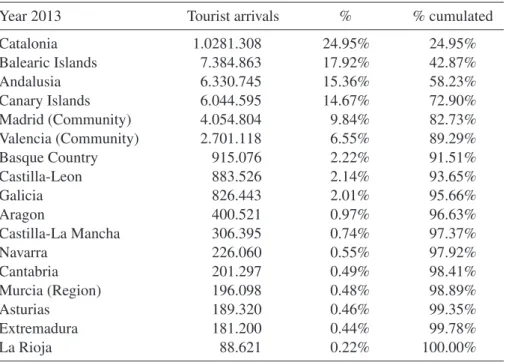
In Table 1 we present the number of international tourist arrivals and the fre-quency distribution of international tourist arrivals in 2013 by region. The main three destinations (Catalonia, the Balearic Islands and Andalusia) account for more than half (59%) of the total number of tourist arrivals to Spain. The first six destinations account for almost 90% of the total number of tourist arrivals, which corroborates that tourism demand is highly concentrated in very few regions.
Table 1: DISTRIBUTION OF THE FREQUENCY OF TOURIST ARRIVALS TOSPANISH REGIONS
Year 2013 Tourist arrivals % % cumulated
Catalonia 1.0281.308 24.95% 24.95% Balearic Islands 7.384.863 17.92% 42.87% Andalusia 6.330.745 15.36% 58.23% Canary Islands 6.044.595 14.67% 72.90% Madrid (Community) 4.054.804 9.84% 82.73% Valencia (Community) 2.701.118 6.55% 89.29% Basque Country 915.076 2.22% 91.51% Castilla-Leon 883.526 2.14% 93.65% Galicia 826.443 2.01% 95.66% Aragon 400.521 0.97% 96.63% Castilla-La Mancha 306.395 0.74% 97.37% Navarra 226.060 0.55% 97.92% Cantabria 201.297 0.49% 98.41% Murcia (Region) 196.098 0.48% 98.89% Asturias 189.320 0.46% 99.35% Extremadura 181.200 0.44% 99.78% La Rioja 88.621 0.22% 100.00%
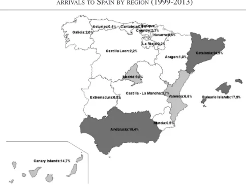
In Figure 1 we map the frequency distribution of international tourist arrivals to Spain by region. The first six destinations are marked in grey. We can see that all these regions, with the exception of Madrid, are located in coastal areas of the Mediterranean, showing the asymmetric concentration of tourism.
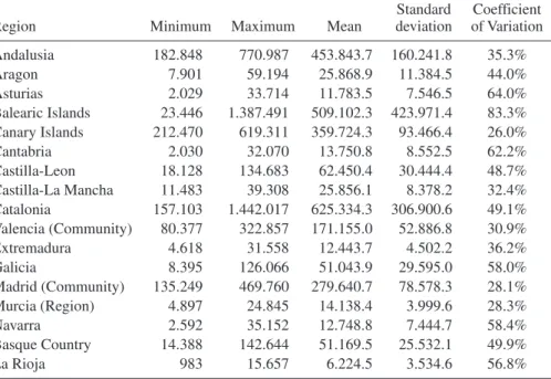
Table 2 presents a descriptive analysis of the data. The Balearic Islands and Cata -lonia are the two regions with the highest peaks. While the Balearic Islands is the region with the highest dispersion in the arrival of tourists, the Canary Islands pre-sent the lowest coefficient of variation (CV), also known as relative standard devi-ation, which is a dimensionless measure of dispersion obtained as the ratio of the standard deviation to the mean and expressed as a percentage. This result may in part be explained by weather conditions, as in the the climate is mild and temperatures remain virtually constant throughout the year.
The performance of the different models is assessed by means of an iterated multi-step ahead forecasting comparison. In order to be able to characterize correctly the performance of the ML methods, and to adjust the hyperparameters and the struc-ture of the models, the database is divided into three subsets:
– Training – From 1999:01 to 2006:12 – Validation – From 2007:01 to 2011:12 – Test – From 2012:01 to 2014:01
In applying ARMA models, only two subsets are used: the in-sample (from 1999:01 to 2011:12) and the out-of-sample periods (from 2012:01 to 2014:01). Ini-tially, the first 52% monthly observations are selected as the training set, the next 33% as the validation set, and the last 15% as the test set. Note that the different sets do not overlap in time.
Figure 1: MEAN ANNUAL GROWTH RATE OF TOURIST ARRIVALS TOSPAIN BY REGION(1999-2013)
The validation set is used to adjust the different parameters of the ML models. In the case of NNs, the validation set is used to determine the optimal stopping time for the training, and the topology of the network. In the case of SVR models, the val-idation set is used for selecting the hyperparameters. The test set is used to estimate the performance of forecasting models on unseen data (Bishop, 1995; Ripley, 1996). After the first step, the partition between train and test sets is done sequentially: as the prediction advances, forecasts are successively incorporated to the training database, leaving the validation set fixed. Therefore, for each forecast, the size of the test set decreases by one period, while the size of the training set increases by one period. In each iteration, models are retrained, and both the optimal structure and the parameters are obtained from the validation set.
The forecasting accuracy of a SVR model depends in good measure on the value of the hyperparameters. Therefore, given the size of the sample, we do an exhaustive enumeration of all possible combinations to estimate the value of the hyperparameters, using as a selection criterion the performance on the validation set at each step.
Regarding the NN models, once the topology of the models is specified, the es-timation of the weights of the networks can be done by means of different algorithms. To avoid the possibility that the search for the optimum value of the parameters fin-ishes in a local minimum, we use a multi-starting technique that initializes the NNs several times for different initial random values, trains the network and chooses the one with the best result on a validation database. All models are implemented using the ‘Scikit-learn’ Python module, which is an open source library that integrates a wide range of state-of-the-art ML algorithms (Pedregosa et al., 2011).
Table 2: DESCRIPTIVE ANALYSIS OF FOREIGN TOURIST ARRIVALS(1999:01-2014:03) Standard Coefficient Region Minimum Maximum Mean deviation of Variation Andalusia 182.848 770.987 453.843.7 160.241.8 35.3% Aragon 7.901 59.194 25.868.9 11.384.5 44.0% Asturias 2.029 33.714 11.783.5 7.546.5 64.0% Balearic Islands 23.446 1.387.491 509.102.3 423.971.4 83.3% Canary Islands 212.470 619.311 359.724.3 93.466.4 26.0% Cantabria 2.030 32.070 13.750.8 8.552.5 62.2% Castilla-Leon 18.128 134.683 62.450.4 30.444.4 48.7% Castilla-La Mancha 11.483 39.308 25.856.1 8.378.2 32.4% Catalonia 157.103 1.442.017 625.334.3 306.900.6 49.1% Valencia (Community) 80.377 322.857 171.155.0 52.886.8 30.9% Extremadura 4.618 31.558 12.443.7 4.502.2 36.2% Galicia 8.395 126.066 51.043.9 29.595.0 58.0% Madrid (Community) 135.249 469.760 279.640.7 78.578.3 28.1% Murcia (Region) 4.897 24.845 14.138.4 3.999.6 28.3% Navarra 2.592 35.152 12.748.8 7.444.7 58.4% Basque Country 14.388 142.644 51.169.5 25.532.1 49.9% La Rioja 983 15.657 6.224.5 3.534.6 56.8%
4. EMPIRICAL RESULTS
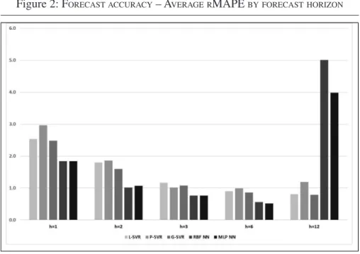
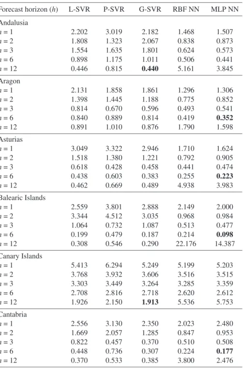
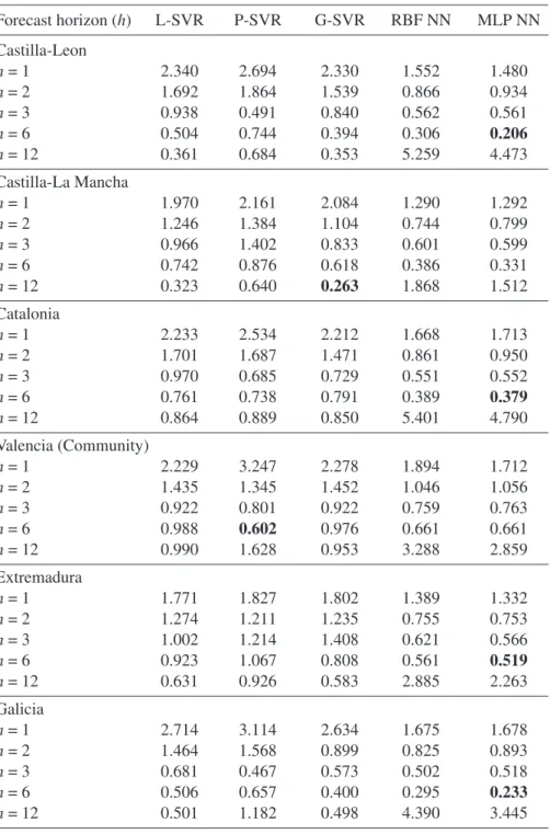
The forecasting performance of the different models is assessed for different time horizons (1, 3, 6 and 12 months) by computing several accuracy measures. First, we obtain the Relative Mean Absolute Percentage Error (rMAPE) statistic for all re-gions (Table 3). The rMAPE ponders the MAPE of the model under evaluation against the MAPE of the benchmark model. We use an ARMA model as a baseline. We find that the lowest rMAPE values are obtained for longer forecast horizons, except for NN models (Figure 2). This result indicates that SVR models improve their forecasting performance with respect to ARMA models as forecast horizons increase. With the exception of the Canary Islands and Madrid, which are the only two regions that do not present a seasonal pattern, in most regions NN models outperform lin-ear models for two, three and six-step ahead forecasts, while SVR models for three, six and twelve-step ahead predictions (Figure 2).
Figure 2: FORECAST ACCURACY– AVERAGE RMAPE BY FORECAST HORIZON
Source: Own elaboration.
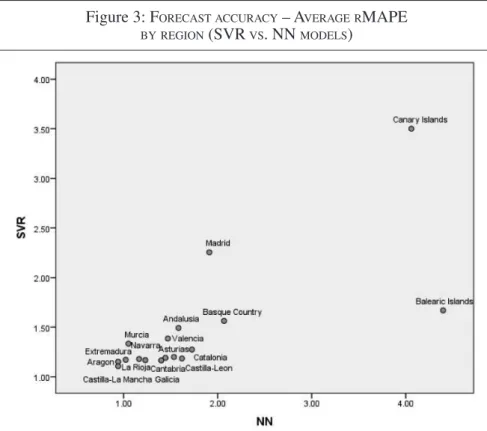
In Figure 3 we map the different regions regarding the average rMAPE. We compare the mean rMAPE values of SVR models to those of NN models, regard-less of the forecast horizon. The highest values are obtained in the Basque Country, Madrid, the Canary Islands and the Balearic Islands. At the other end, Aragon, Castilla-La Mancha and La Rioja present the lowest average rMAPE values, indi-cating the regions where, on average, ML models show the best forecasting perfor-mance with respect to ARMA models.
Table 3: FORECAST ACCURACY. RELATIVEMAPE (2013:03-2014:01) – ML VS. ARMA MODELS Forecast horizon (h) L-SVR P-SVR G-SVR RBF NN MLP NN Andalusia h= 1 2.202 3.019 2.182 1.468 1.507 h= 2 1.808 1.323 2.067 0.838 0.873 h= 3 1.554 1.635 1.801 0.624 0.573 h= 6 0.898 1.175 1.011 0.506 0.441 h= 12 0.446 0.815 0.440 5.161 3.845 Aragon h= 1 2.131 1.858 1.861 1.296 1.306 h= 2 1.398 1.445 1.188 0.775 0.852 h= 3 0.814 0.670 0.596 0.493 0.541 h= 6 0.840 0.889 0.814 0.419 0.352 h= 12 0.891 1.010 0.876 1.790 1.598 Asturias h= 1 3.049 3.322 2.946 1.710 1.624 h= 2 1.518 1.380 1.221 0.792 0.905 h= 3 0.618 0.428 0.458 0.441 0.474 h= 6 0.438 0.603 0.383 0.255 0.223 h= 12 0.462 0.669 0.489 4.938 3.983 Balearic Islands h= 1 2.559 3.801 2.888 2.149 2.000 h= 2 3.344 4.512 3.035 0.968 0.984 h= 3 1.064 0.732 1.087 0.513 0.477 h= 6 0.199 0.479 0.187 0.214 0.098 h= 12 0.308 0.546 0.290 22.176 14.387 Canary Islands h= 1 5.413 6.294 5.249 5.199 5.203 h= 2 3.768 3.932 3.606 3.516 3.515 h= 3 3.303 3.449 3.264 3.285 3.359 h= 6 2.708 2.816 2.718 2.620 2.612 h= 12 1.926 2.150 1.913 5.536 5.753 Cantabria h= 1 2.556 3.130 2.350 2.023 2.480 h= 2 1.669 2.057 1.285 0.847 0.953 h= 3 0.822 0.457 0.370 0.510 0.508 h= 6 0.448 0.736 0.307 0.224 0.177 h= 12 0.370 0.533 0.385 3.800 2.476
Table 3: FORECAST ACCURACY. RELATIVEMAPE (2013:03-2014:01) – ML VS. ARMA MODELS(continuation)
Forecast horizon (h) L-SVR P-SVR G-SVR RBF NN MLP NN Castilla-Leon h= 1 2.340 2.694 2.330 1.552 1.480 h= 2 1.692 1.864 1.539 0.866 0.934 h= 3 0.938 0.491 0.840 0.562 0.561 h= 6 0.504 0.744 0.394 0.306 0.206 h= 12 0.361 0.684 0.353 5.259 4.473 Castilla-La Mancha h= 1 1.970 2.161 2.084 1.290 1.292 h= 2 1.246 1.384 1.104 0.744 0.799 h= 3 0.966 1.402 0.833 0.601 0.599 h= 6 0.742 0.876 0.618 0.386 0.331 h= 12 0.323 0.640 0.263 1.868 1.512 Catalonia h= 1 2.233 2.534 2.212 1.668 1.713 h= 2 1.701 1.687 1.471 0.861 0.950 h= 3 0.970 0.685 0.729 0.551 0.552 h= 6 0.761 0.738 0.791 0.389 0.379 h= 12 0.864 0.889 0.850 5.401 4.790 Valencia (Community) h= 1 2.229 3.247 2.278 1.894 1.712 h= 2 1.435 1.345 1.452 1.046 1.056 h= 3 0.922 0.801 0.922 0.759 0.763 h= 6 0.988 0.602 0.976 0.661 0.661 h= 12 0.990 1.628 0.953 3.288 2.859 Extremadura h= 1 1.771 1.827 1.802 1.389 1.332 h= 2 1.274 1.211 1.235 0.755 0.753 h= 3 1.002 1.214 1.408 0.621 0.566 h= 6 0.923 1.067 0.808 0.561 0.519 h= 12 0.631 0.926 0.583 2.885 2.263 Galicia h= 1 2.714 3.114 2.634 1.675 1.678 h= 2 1.464 1.568 0.899 0.825 0.893 h= 3 0.681 0.467 0.573 0.502 0.518 h= 6 0.506 0.657 0.400 0.295 0.233 h= 12 0.501 1.182 0.498 4.390 3.445
Table 3: FORECAST ACCURACY. RELATIVEMAPE (2013:03-2014:01) – ML VS. ARMA MODELS(continuation)
Forecast horizon (h) L-SVR P-SVR G-SVR RBF NN MLP NN Madrid (Community) h= 1 2.752 3.625 2.687 2.323 2.056 h= 2 1.941 2.179 1.866 1.340 1.213 h= 3 1.900 1.175 1.922 1.225 1.155 h= 6 1.927 1.867 1.917 0.995 0.928 h= 12 2.061 3.888 2.123 4.123 3.757 Murcia (Region) h= 1 2.010 2.021 1.961 1.460 1.489 h= 2 1.342 1.281 1.172 0.908 0.989 h= 3 1.080 0.953 1.042 0.708 0.746 h= 6 1.204 1.016 1.210 0.724 0.762 h= 12 1.135 1.502 1.063 1.435 1.288 Navarra h= 1 2.251 2.573 2.178 1.590 1.582 h= 2 1.365 1.634 1.254 0.775 0.853 h= 3 0.803 0.670 0.702 0.462 0.470 h= 6 0.697 0.912 0.564 0.303 0.245 h= 12 0.562 0.796 0.558 3.189 2.827 Basque Country h= 1 2.189 2.250 2.130 1.551 1.776 h= 2 2.031 1.893 1.790 0.850 0.934 h= 3 1.408 1.270 1.242 0.560 0.574 h= 6 0.863 0.730 0.944 0.467 0.466 h= 12 1.516 1.707 1.486 7.005 6.491 La Rioja h= 1 2.679 3.024 2.409 1.161 1.166 h= 2 1.591 0.979 1.010 0.664 0.709 h= 3 0.956 0.727 0.555 0.529 0.520 h= 6 0.740 0.973 0.515 0.276 0.227 h= 12 0.387 0.667 0.346 2.972 1.999
Note: The rMAPE ponders the MAPE of the model under evaluation against the MAPE of the benchmark model. We use an ARMA model as a baseline. Best model for each region in bold.
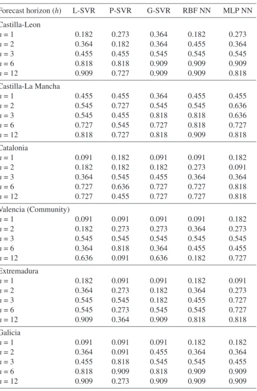
To attain a more comprehensive forecasting evaluation, we compute the PLAE statistic proposed by Claveria et al.(2015b). The PLAE gives the proportion of out-of-sample periods with lower absolute forecast errors than a benchmark model (Table 4). The PLAE is a dimensionless measure based on the CJ statistic for mar-ket efficiency (Cowles and Jones, 1937):
Figure 3: FORECAST ACCURACY– AVERAGE RMAPE BY REGION(SVR VS. NN MODELS)
Source: Own elaboration.
∑
λ = = PLAE n t t n 1 λ =⎧ < ⎨ ⎪ ⎩⎪ e e 1 if 0 otherwise t t A, t B, [10] whereWhere ytis the actual value, and yˆtthe forecasted value at period t= 1, ... n. Fore-cast errors can then be defined as et= yt–yˆt. Given two competing models A and B, where A refers to the forecasting model under evaluation and B stands for the benchmark model. In this study we use the ARMA model as a baseline.
In Table 4 we can observe a similar pattern to the one obtained with the rMAPE. Results show that the G-SVR is the method that outperforms the ARMA model in more cases. Special mention should be made of the Canary Islands and the Com-munity of Madrid, where in most cases no ML method outperforms the ARMA.
Table 4: FORECAST ACCURACY. PLAE (2013:03-2014:01) – ML VS. ARMA MODELS Forecast horizon (h) L-SVR P-SVR G-SVR RBF NN MLP NN Andalusia h= 1 0.182 0.091 0.091 0.091 0.091 h= 2 0.364 0.364 0.182 0.273 0.182 h= 3 0.455 0.455 0.364 0.364 0.364 h= 6 0.545 0.364 0.364 0.273 0.455 h= 12 0.818 0.455 0.818 0.818 0.727 Aragon h= 1 0.091 0.182 0.182 0.182 0.182 h= 2 0.273 0.273 0.273 0.455 0.273 h= 3 0.455 0.545 0.545 0.455 0.455 h= 6 0.727 0.545 0.727 0.727 0.818 h= 12 0.636 0.364 0.636 0.636 0.818 Asturias h= 1 0.000 0.091 0.091 0.182 0.182 h= 2 0.182 0.273 0.364 0.364 0.364 h= 3 0.545 0.636 0.727 0.455 0.636 h= 6 0.909 0.818 0.818 0.909 0.909 h= 12 0.818 0.636 0.818 0.727 0.818 Balearic Islands h= 1 0.182 0.182 0.364 0.273 0.273 h= 2 0.091 0.091 0.455 0.273 0.273 h= 3 0.455 0.545 0.636 0.545 0.545 h= 6 1.000 0.909 1.000 1.000 0.818 h= 12 1.000 0.818 1.000 1.000 0.818 Canary Islands h= 1 0.000 0.000 0.000 0.000 0.000 h= 2 0.091 0.000 0.091 0.000 0.091 h= 3 0.000 0.000 0.000 0.000 0.000 h= 6 0.000 0.000 0.000 0.000 0.000 h= 12 0.000 0.000 0.000 0.000 0.000 Cantabria h= 1 0.000 0.273 0.273 0.182 0.182 h= 2 0.273 0.182 0.545 0.273 0.364 h= 3 0.727 0.818 0.727 0.636 0.636 h= 6 0.818 0.636 0.909 0.909 0.909 h= 12 0.909 0.727 0.909 0.818 0.909
Table 4: FORECAST ACCURACY. PLAE
(2013:03-2014:01) – ML VS. ARMA MODELS(continuation)
Forecast horizon (h) L-SVR P-SVR G-SVR RBF NN MLP NN Castilla-Leon h= 1 0.182 0.273 0.364 0.182 0.273 h= 2 0.364 0.182 0.364 0.455 0.364 h= 3 0.455 0.455 0.545 0.545 0.545 h= 6 0.818 0.818 0.909 0.909 0.909 h= 12 0.909 0.727 0.909 0.909 0.818 Castilla-La Mancha h= 1 0.455 0.455 0.364 0.455 0.455 h= 2 0.545 0.727 0.545 0.545 0.636 h= 3 0.545 0.455 0.818 0.818 0.636 h= 6 0.727 0.545 0.727 0.818 0.727 h= 12 0.818 0.727 0.818 0.909 0.818 Catalonia h= 1 0.091 0.182 0.091 0.091 0.182 h= 2 0.182 0.182 0.182 0.273 0.091 h= 3 0.364 0.545 0.455 0.364 0.364 h= 6 0.727 0.636 0.727 0.727 0.818 h= 12 0.727 0.455 0.727 0.727 0.818 Valencia (Community) h= 1 0.091 0.091 0.091 0.091 0.182 h= 2 0.182 0.273 0.273 0.364 0.273 h= 3 0.545 0.545 0.545 0.545 0.545 h= 6 0.364 0.818 0.364 0.455 0.455 h= 12 0.636 0.091 0.636 0.182 0.727 Extremadura h= 1 0.182 0.091 0.091 0.182 0.091 h= 2 0.364 0.273 0.182 0.364 0.273 h= 3 0.545 0.545 0.182 0.455 0.727 h= 6 0.545 0.273 0.545 0.545 0.727 h= 12 0.909 0.364 0.909 0.818 0.818 Galicia h= 1 0.091 0.091 0.091 0.182 0.182 h= 2 0.364 0.091 0.455 0.364 0.364 h= 3 0.455 0.818 0.545 0.545 0.455 h= 6 0.818 0.909 0.818 0.909 0.909 h= 12 0.909 0.273 0.909 0.909 0.909
Table 4: FORECAST ACCURACY. PLAE
(2013:03-2014:01) – ML VS. ARMA MODELS(continuation)
Forecast horizon (h) L-SVR P-SVR G-SVR RBF NN MLP NN Madrid (Community) h= 1 0.091 0.091 0.182 0.091 0.182 h= 2 0.273 0.273 0.273 0.273 0.273 h= 3 0.182 0.545 0.182 0.182 0.182 h= 6 0.182 0.182 0.182 0.182 0.273 h= 12 0.000 0.000 0.000 0.182 0.182 Murcia (Region) h= 1 0.091 0.182 0.091 0.182 0.364 h= 2 0.273 0.182 0.455 0.273 0.455 h= 3 0.273 0.455 0.364 0.364 0.364 h= 6 0.364 0.364 0.364 0.182 0.364 h= 12 0.455 0.182 0.636 0.545 0.636 Navarra h= 1 0.091 0.000 0.091 0.182 0.091 h= 2 0.273 0.182 0.273 0.273 0.273 h= 3 0.455 0.545 0.636 0.455 0.455 h= 6 0.727 0.455 0.727 0.636 0.818 h= 12 0.727 0.455 0.727 0.636 0.818 Basque Country h= 1 0.182 0.091 0.182 0.182 0.000 h= 2 0.182 0.273 0.182 0.273 0.182 h= 3 0.455 0.364 0.364 0.364 0.455 h= 6 0.545 0.636 0.545 0.545 0.636 h= 12 0.091 0.091 0.091 0.273 0.091 La Rioja h= 1 0.273 0.000 0.182 0.182 0.182 h= 2 0.273 0.364 0.455 0.182 0.182 h= 3 0.545 0.727 0.545 0.636 0.636 h= 6 0.636 0.455 0.818 0.818 0.818 h= 12 0.727 0.545 0.818 0.636 0.909
Note: The PLAE ratio measures the proportion of out-of-sample periods with lower absolute errors than the baseline model (ARMA model). Values below 0.5 indicate that the baseline model dis-plays a higher number of lower absolute forecast errors than the model under evaluation for the out-of-sample period.
To test whether the reduction in MAPE is statistically significant between the best three models, in Table 5 we present the results of the Diebold-Mariano (DM) statis-tic of predictive accuracy (Diebold and Mariano, 1995). The null hypothesis of the test is that the difference between the two competing series is non-significant. A neg-ative sign of the statistic implies that the second model has bigger forecasting errors.
Table 5: DM LOSS-DIFFERENTIAL TEST STATISTIC FOR PREDICTIVE ACCURACY 12 months ahead forecasts G-SVR vs. P-SVR G-SVR vs. MLP NN
Andalusia -4.004 -1.728 Aragon -1.590 0.819 Asturias -2.596 -0.083 Balearic Islands -1.408 -1.728 Canary Islands -2.318 2.365 Cantabria -1.604 -0.476 Castilla-Leon -4.432 -1.157 Castilla-La Mancha -1.692 -2.022 Catalonia -1.164 0.588 Valencia (Community) -5.674 0.944 Extremadura -3.136 -0.388 Galicia -6.461 0.503 Madrid (Community) -11.628 -0.834 Murcia (Region) -2.184 0.672 Navarra -3.682 0.051 Basque Country -2.903 -0.278 La Rioja -2.490 -1.063
Note: Diebold-Mariano test statistic with NW estimator. Null hypothesis: the difference between the two competing series is non-significant. A negative sign of the statistic implies that the second model (P-SVR, MLP NN) has bigger forecasting errors. The 5% level critical value is 2.028. Sig-nificant values in bold.
When comparing the forecast accuracy of the G-SVR against that of the other two models that yielded the lowest MAPE values, we find that the G-SVR shows a significant improvement over the P-SVR in most regions, but the improvements over the MLP NN are not significant.
These results confirm previous research by Hong (2006) and Chen and Wang (2007), who obtain better forecasting results with SVM-based models than with NNs for tourist arrivals to Barbados and China respectively. Velásquez et al. (2010) also obtain better predictions with SVMs than with MLP NNs. Notwithstanding, we find that the improvements in terms of MAPE of SVR models with respect to MLP net-works are not statistically significant.
Finally in Table 6 we present a summary of the MAPE values. The results show that while linear models are preferable for short-term forecasting, ML techniques are more suitable for long-term prediction. From three-month ahead on, both SVR and NN models outperform ARMA models. In this experiment all ML techniques have been specified so as to use only one temporal lag for concatenation, as opposed to linear models which were set to select the optimal number of AR and MA terms by means of the Akaike information criterion (AIC). The implementation of a model criterion to identify the best suited specification regarding the number of lags in ML methods would allow to perform equivalent forecasting comparisons to linear models.
Table 6: FORECAST ACCURACY– SUMMARY OFMAPE VALUES BY TECHNIQUE
Forecast horizon (h) Mean Median
Linear models (ARMA models)
h= 1 0.325 0.200
h= 2 0.472 0.315
h= 3 0.713 0.425
h= 6 0.727 0.457
h= 12 0.661 0.349
Support Vector Regression (SVR models)
h= 1 0.903 0.464
h= 2 0.974 0.473
h= 3 0.619 0.401
h= 6 0.416 0.360
h= 12 0.402 0.318
Neural Networks (RBF and MLP)
h= 1 0.655 0.420
h= 2 0.751 0.428
h= 3 0.707 0.413
h= 6 0.424 0.342
h= 12 0.389 0.299
Note: Lowest values for each type of technique in bold.
To summarize, the overall forecasting performance of all methods improves for longer forecast horizons. Regarding the different techniques we obtain slightly bet-ter predictions with SVR models than with NNs. Nevertheless, not all SVRs show the same performance. The SVR with a Gaussian RBF kernel outperforms the rest of the models, especially for mid and long-term forecasts. This result is indicative that the data is clustered along the margins that surround the regression function in
the SVR model. The fact that the data is clustered instead of spread in the input space, also explains the lower performance of the polynomial kernel.
As Gaussian RBF kernels are the most prevalent choice for SVR-based fore-casting (Smola and Schölkopf, 1998), and are also easy to implement, our results sug-gest the potential of this SVR model for tourism demand forecasting. These findings also highlight the importance of properly selecting the kind of kernel function when using SVR models with forecasting purposes.
5. SUMMARY AND CONCLUSIONS
As more accurate predictions become essential for effective policy planning, new forecasting methods provide room for improvement. Artificial intelligence methods based on machine learning such as Support Vector Regressions and Artificial Neural Networks have attracted increasing interest to refine the predictions in the tourism industry. SVR and NN are flexible techniques that admit a wide array of models. The main purpose of this study is to assess the forecasting performance of Support Vec-tor Regression for tourism demand prediction and seasonal forecasting. With this aim we assess the influence on the prediction accuracy of the different techniques as fore-cast horizons increase.
Three different SVR models based on different kernel functions and two alternative NN architectures have been used to generate predictions of international tou -rism demand to all seventeen regions of Spain. By means of several forecast accu-racy measures, the different ML techniques have been evaluated with respect to a linear model used as a baseline. The forecasting out-of-sample comparison shows that the SVR with a Gaussian RBF kernel outperforms the rest of the models in most cases. The statistically significant improvement in terms of forecast accuracy with respect to other SVR models illustrates the importance of not overlooking the pa-rameter and kernel function selection for SVR modeling.
Another interesting finding is that ML methods improve their forecasting per-formance with respect to linear stochastic models as forecast horizons increase. While NN models show the best performance for intermediate forecast horizons, SVR mod-els tend to yield the best predictions for the longer time horizons. This result sug-gests that the optimal forecasting methodology depends on the time horizon of the predictions. In this sense future research should focus on developing a model se-lection criterion dependent on different forecast horizons.
This research contributes to the economic literature and to the tourism indus-try by shedding some light on the most appropriate SVR model to predict seasonal time series and tourism demand. A question that requires to be examined in further detail is the implementation of model selection criteria for ML techniques that would allow to refine AI-based predictions. The comparison of SVR to alternative ML tech-niques such as Gaussian process regression is also left for future research.
E
A
REFERENCES
Aguiló, E., Riera, A. and Rosselló, J. (2005): The short-term price effect of a tourist tax through a dynamic demand model: The Case of the Balearic Islands. Tourism Management,n. 26, pp. 359-365.
Álvarez-Díaz, M. and Rosselló-Nadal, J. (2010): Forecasting British tourist arrivals in the Balearic Islands using meteorological variables. Tourism Economics,n. 16, pp. 153-168. Akin, M. (2015): A novel approach to model selection in tourism demand modeling. Tourism
Management, n. 48, pp. 64-72.
Andrades-Caldito, L., Sánchez-Rivero, M. and Pulido-Fernández, J.I. (2013): Differentiating Competitiveness through Tourism Image Assessment. An Application to Andalusia (Spain). Journal of Travel Research,n. 52, pp. 68-81.
Assaf, A.G., Barros, C.P. and Gil-Alana, L.A. (2011): Persistence in the Short- and Long-Term Tourist Arrivals to Australia. Journal of Travel Research,n. 50, pp. 213-229.
Bardolet, E. and Sheldon, P.J. (2008): Tourism in Archipelagos and the Balearics. Annals of Tourism Research,n. 35, pp. 900-923.
Bishop, C.M. (1995): Neural Networks for Pattern Recognition. Oxford University Press: Ox-ford.
Burger, C., Dohnal, M., Kathrada, M. and Law, R. (2001): A practitioners guide to time-series methods for tourism demand forecasting: A case study of Durban, South Africa. Tourism Management,n. 22, pp. 403-409.
Burges, C.J.C. (1988): A Tutorial on Support Vector Machines for Pattern Recognition. Data Mining and Knowledge Discovery,n. 2, pp. 121-167.
Cang, S. (2014): A Comparative Analysis of Three Types of Tourism Demand Forecasting Models: Individual, Linear Combination and Non-Linear Combination. International Journal of Tourism Research,n. 16, pp. 596-607.
Cao, L. (2003): Support Vector Machines Experts for Time Series Forecasting. Neurocom-puting,n. 51, pp. 321-339.
Chen, K.Y. and Wang, C.H. (2007): Support Vector Regression with Genetic Algorithms in Forecasting Tourism Demand. Tourism Management,n. 28, pp. 215-226.
Chen, W.H., Shih, J.Y. and Wu, S. (2006): Comparison of Support-Vector Machines and Back Propagation Neural Networks in Forecasting the Six Major Asian Stock Markets. Inter-national Journal of Electronic Finance,n. 1, pp. 49-67.
Chu, F.L. (2009): Forecasting tourism demand with ARMAbased methods. Tourism Mana -gement,n. 30, pp. 740-751.
Claveria, O. and Torra, S. (2014): Forecasting Tourism Demand to Catalonia: Neural Networks vs. Time Series Models. Economic Modelling,n. 36, pp. 220-228.
Claveria, O., Monte, E. and Torra, S. (2015a): Tourism Demand Forecasting with Neural Net-works Models: Different Ways of Treating Information. International Journal of Tourism Research, n. 17, pp. 492-500.
Claveria, O., Monte, E. and Torra, S. (2015b): A New Forecasting Approach for the Hospi-tality Industry. International Journal of Contemporary HospiHospi-tality Management,n. 27, pp. 1520-1538.
Claveria, O., Monte, E. and Torra, S. (2016): Data Pre-Processing for Neural Network-based Forecasting: Does it Really Matter? Technical and Economic Development of Economy, Forthcoming.
Cortes, C. and Vapnik, V. (1995): Support-Vector Networks. Machine Learning,n. 20, pp. 273-297.
Cortés-Jiménez, I. and Blake, A. (2011): Tourism Demand Modeling by Purpose of Visit and Nationality. Journal of Travel Research,n. 50, pp. 408-416.
Cowles, A. and Jones, H. (1937): Some A Posteriori Probabilities in Stock Market Action. Econometrica,n. 5, pp. 280-294.
Cristianini, N. and Shawe-Taylor, J. (2000): An Introduction to Support Vector Machines and Other Kernel-based Learning Methods. Cambridge University Press: Cambridge. Çuhadar, M., Cogurcu, I. and Kukrer, C. (2014): Modelling and Forecasting Cruise Tourism
Demand to zmir by Different Artificial Neural Network Architectures. International Jour-nal of Business and Social Research,n. 4, pp. 12-28.
Diebold, F.X. and Mariano, R. (1995): Comparing predictive accuracy. Journal of Business and Economic Statistics,n. 13, pp. 253-263.
Drucker, H., Burges, C.J.C., Kaufman, L., Smola, A. and Vapnik, V. (1997): Support Vector Regression Machines. In: M. Mozer, M. Jordan and T. Petsche (eds.), Advances in Neural Information Processing Systems, vol. 9 (pp. 155-161). MIT Press: Cambridge, MA. Garín-Muñoz, T. and Montero-Martín, L.F. (2007): Tourism in the Balearic Islands: A dynamic
model for international demand using panel data. Tourism Management,n. 28, pp. 1224-1235. Gil-Alana, L.A., Cunado, J. and De Gracia, F.P. (2008): Tourism in the Canary Islands: Fore-casting Using Several Seasonal Time Series Models. Journal of ForeFore-casting,n. 27, pp. 621-636.
Goh, C., Law, R. and Mok, H.M. (2008): Analyzing and Forecasting Tourism Demand: A Rough Sets Approach. Journal of Travel Research,n. 46, pp. 327-338.
Gounopoulos, D., Petmezas, D. and Santamaria, D. (2012): Forecasting Tourist Arrivals in Greece and the Impact of Macroeconomic Shocks from the Countries of Tourists’ Origin. Annals of Tourism Research,n. 39, pp. 641-666.
Gunter, U. and Önder, I. (2015): Forecasting International City Tourism Demand for Paris: Accuracy of Uni- and Multivariate Models Employing Monthly Data. Tourism Manage-ment,n. 46, pp. 123-135.
Guo, X., Sun, L., Li, G. and Wang, S. (2008): A Hybrid Wavelet Analysis and Support Vec-tor Machines in Forecasting Development of Manufacturing. Expert Systems with Ap-plications,n. 35, pp. 415-422.
Hassani, H., Webster, A., Silva, E.S. and Heravi, S. (2015): Forecasting U.S. Tourist Arrivals Using Optimal Singular Spectrum Analysis. Tourism Management,n. 46, pp. 322-335. Hastie, T., Tibshirani, R. and Friedman, J. (2009): The Elements of Statistical Learning. Data
Mining, Inference and Prediction. Springer: New York.
Haykin, S. (2008): Neural Networks and Learning Machines(3rd Edition). Prentice Hall: New Jersey.
Hernández-López, M. and Cáceres-Hernández, J.J. (2007): Forecasting Tourists’ Character-istics by a Genetic Algorithm with a Transition Matrix. Tourism Management,n. 28, pp. 290-297.
Hong, W.C. (2006): The Application of Support Vector Machines to Forecast Tourist Arrivals in Barbados: an Empirical Study. International Journal of Management,n. 23, pp. 375-385. Hong, W.C. (2011): Traffic Flow Forecasting by Seasonal SVR with Chaotic Simulated
An-nealing Algorithm. Neurocomputing,n. 74, pp. 2096-2107.
Hong, W., Dong, Y., Chen, L. and Wei, S. (2011): SVR with Hybrid Chaotic Genetic Algo-rithms for Tourism Demand Forecasting. Applied Soft Computing,n. 11, pp. 1881-1890. Huang, W., Nakamori, Y. and Wang, S.Y. (2005): Forecasting Stock Market Movement Direc-tion with Support Vector Machine. Computers & OperaDirec-tions Research,n. 32, pp. 2513-2522. Kim, K. (2003): Financial Time Series Forecasting Using Support Vector Machines.
Kim, D. and Schwartz, Y. (2013): The Accuracy of Tourism Forecasting and Data Charac-teristics: A Meta-analytical Approach. Journal of Hospitality Marketing and Management, n. 22, pp. 349-374.
Kon, S. and Turner, L.L. (2005): Neural Network Forecasting of Tourism Demand. Tourism Economics,n. 11, pp. 301-328.
Lehmann, R. and Wohlrabe, K. (2015): Forecasting GDP at the Regional Level with Many Predictors. German Economic Review,n. 16, pp. 226-254.
Li, H. and Sun, J. (2012): Forecasting Business Failure: The Use of Nearest-neighbour Sup-port Vectors and Correcting Imbalanced Samples – Evidence from the Chinese Hotel In-dustry. Tourism Management,n. 33, pp. 622-634.
Li, G., Song, H., Cao, Z. and Wu, D.C. (2013): How Competitive is Hong Kong against its Competitors? An Econometric Study. Tourism Management,n. 36, pp. 247-256. Lin, H.L., Liu, M.L., Tseng, Y.H. and Su, Y.W. (2011): Taiwan’s International Tourism: A Time
Series Analysis with Calendar Effects and Joint Outlier Adjustments. International Jour-nal of Tourism Research,n. 13, pp. 1-16.
Medeiros, M.C., McAleer, M., Slottje, D., Ramos, V. and Rey-Maquieira, J. (2008): An Al-ternative Approach to Estimating Demand: Neural Network Regression with Condi-tional Volatility for High Frequency Air Passenger Arrivals. Journal of Econometrics,n. 147, pp. 372-383.
Molinet, T., Molinet, J.A., Betancourt, M.E., Palmer, A. and Montaño, J.J. (2015): Models of Artificial Neural Networks Applied to Demand Forecasting in Nonconsolidated Tourist Destinations. Methodology: European Journal of Research Methods for the Behavioral and Social Sciences. Forthcoming.
Page, S., Song, H. and Wu, D.C. (2012): Assessing the Impacts of the Global Economic Cri-sis and Swine Flu on Inbound Tourism Demand in the United Kingdom. Journal of Travel Research,n. 51, pp. 142-153.
Pai, P.F. and Hong, W.C. (2005): An Improved Neural Network Model in Forecasting Arrivals. Annals of Tourism Research,n. 32, pp. 1138-1141.
Pai, P.F. and Hong, W.C. (2007): A Recurrent Support Vector Regression Model in Rainfall Forecasting. Hydrological Processes,n. 21, pp. 819-827.
Pai, P.F. and Lin, C.S. (2005): A Hybrid ARIMA and Support Vector Machines Model in Stock Price Forecasting. Omega,n. 33, pp. 497-505.
Palmer, A., Montaño, J.J. and Sesé, A. (2006): Designing an Artificial Neural Network for Forecasting Tourism Time-Series. Tourism Management,n. 27, pp. 781-790.
Pattie, D.C. and Snyder, J. (1996): Using a neural network to forecast visitor behavior. An-nals of Tourism Research,n. 23, pp. 151-164.
Pedregosa, F., Varoquaux, G., Gramfort, A., Michel, V., Thirion, B., Grisel, O., Blondel, M., Prettenhofer, P., Weiss, R., Dubourg, V., Vanderplas, J., Passos, A., Cournapeau, D., Bru -cher, M., Perrot, M. and Duchesnay, E. (2011): Scikit-learn: Machine Learning in Python. Journal of Machine Learning Research,n. 12, pp. 2825-2830.
Peng, B., Song, H. and Crouch, G.I. (2014): A Meta-analysis of International Tourism De-mand Forecasting and Implications for Practice. Tourism Management,n. 45, pp. 181-193. Ripley, B.D. (1996): Pattern Recognition and Neural Networks. Cambridge University Press:
Cambridge.
Rosselló-Nadal, J. (2001): Forecasting Turning Points in International Visitor Arrivals in the Balearic Islands. Tourism Economics,n. 7, pp. 365-380.
Santana-Jiménez, Y. and Hernández, J.M. (2011): Estimating the Effect of Overcrowding on Tourist Attraction: The Case of Canary Islands. Tourism Management,n. 32, pp. 415-425.
Sarrión-Gavilán, M.D., Benítez-Márquez, M.D. and Mora-Rangel, E.O. (2015): Spatial dis-tribution of tourism supply in Andalusia. Tourism Management,n. 15, pp. 29-45. Smola, A.J. and Schölkopf, B. (1998): A Tutorial on Support Vector Regression. Royal
Hol-loway College: London, UK.
Song, H. and Li, G. (2008): Tourism Demand Modelling and Forecasting – A Review of Re-cent Research. Tourism Management,n. 29, pp. 203-220.
Tay, Feh and Cao, L. (2001): Application of Support Vector Machines in Financial Time Se-ries Forecasting. Omega,n. 29, pp. 309-317.
Teixeira, J.P. and Fernandes, P.O. (2014): Tourism Time Series Forecast – Different ANN Ar-chitectures with Time Index Input. Procedia Technology,n. 5, pp. 445-454.
Tsaur, R. and Kuo, T. (2011): The Adaptive Fuzzy Time Series Model with an Application to Taiwan’s Tourism Demand. Expert Systems with Applications,n. 38, pp. 9164-9171. Vapnik, V.N. (1995): The Nature of Statistical Learning. Springer-Verlag: New York. Velásquez, J.D., Olaya, Y. and Franco, C.J. (2010): Time Series Prediction Using Support
Vec-tor Machines. Revista Chilena de Ingeniería,n. 18, pp. 64-75.
Wu, Q., Law, R. and Xu, X. (2012): A Spare Gaussian Process Regression Model for Tourism Demand Forecasting in Hong Kong. Expert Systems with Applications,n. 39, pp. 4769-4774. Xu, X., Law, R. and Wu, T. (2009): Support Vector Machines with Manifold Learning and Probabilistic Space Projection for Tourist Expenditure Analysis. International Journal of Computational Intelligence Systems,n. 2, pp. 17-26.
Yu, G. and Schwartz, Z. (2006): Forecasting Short Time-Series Tourism Demand with Arti-ficial Intelligence Models. Journal of Travel Research,n. 45, pp. 194-203.
Zhang, G., Putuwo, B.E. and Hu, M.Y. (1998): Forecasting with Artificial Neural Networks: The State of the Art. International Journal of Forecasting,n. 14, pp. 35-62.
Fecha de recepción del original: Versión final:
RESUMEN
El presente estudio evalúa la influencia de los horizontes predictivos sobre la precisión de las predicciones obtenidas mediante técnicas de inteligencia artificial basadas en aprendizaje automático. Para ello se compara la capa-cidad predictiva de diferentes modelos de Regresión de Soporte Vectorial (RSV) y de Redes Neuronales (RNA) con un modelo lineal utilizado como referencia. El análisis se centra en la demanda de turismo extranjero en Es-paña a nivel regional. La RSV entrenada con un kernel de función de base radial gaussiana supera al resto de modelos para las predicciones a más largo plazo. También se encuentra que los métodos de aprendizaje automático me-joran su capacidad predictiva con respecto a los modelos lineales a medida que aumenta el horizonte de predicción. Este resultado pone de manifiesto la idoneidad de la RSV para la predicción a medio y largo plazo.
Palabras clave: predicción, demanda turística, España, regresión de soporte vectorial, redes neuronales artificiales, técnicas de aprendizaje automático. Clasificación JEL:C02, C22, C45, C63, E27, R11.