Open Access
Proceedings
Time-series alignment by non-negative multiple generalized
canonical correlation analysis
Bernd Fischer*
1,2, Volker Roth
1and Joachim M Buhmann
1,2Address: 1Institute of Computational Science, ETH Zurich, Switzerland and 2Competence Center of Systems Physiology and Metabolic Diseases, ETH Zurich, Switzerland
Email: Bernd Fischer* - [email protected]; Volker Roth - [email protected]; Joachim M Buhmann - [email protected] * Corresponding author
Abstract
Background: Quantitative analysis of differential protein expressions requires to align temporal
elution measurements from liquid chromatography coupled to mass spectrometry (LC/MS). We propose multiple Canonical Correlation Analysis (mCCA) as a method to align the non-linearly distorted time scales of repeated LC/MS experiments in a robust way.
Results: Multiple canonical correlation analysis is able to map several time series to a consensus
time scale. The alignment function is learned in a supervised fashion. We compare our approach with previously published methods for aligning mass spectrometry data on a large proteomics dataset. The proposed method significantly increases the number of proteins that are identified as being differentially expressed in different biological samples.
Conclusion: Jointly aligning multiple liquid chromatography/mass spectrometry samples by mCCA
substantially increases the detection rate of potential bio-markers which significantly improves the interpretability of LC/MS data.
Background
Liquid chromatography coupled to mass spectrometry (LC/MS) has emerged as the technology of choice for the quantitative analysis of proteins over the last decade. Technically, the liquid chromatography process separates solute molecules of a multi component chemical mixture which are measured by LC detectors as a time series of sol-ute mass. A major problem when comparing two biologi-cal samples measured with LC/MS is a non-linear deformation of the time scale between two experiments. A LC/MS device generates mass peaks along the time axis.
When two mass spectrometry experiments are aligned, it is our goal to generate matching hypotheses for as many peaks as possible between the two runs, while ensuring that most of these hypotheses are correct.
One of the standard methods for aligning mass spectrom-etry experiments is called correlation optimized warping
(COW) [1], where piece-wise linear functions are fitted to align pairs of time series. A hidden Markov model [2] was proposed to align the mass spectrometry data as well as acoustic time series. In [3] the model was extended to use
from NIPS workshop on New Problems and Methods in Computational Biology Whistler, Canada. 8 December 2006
Published: 21 December 2007
BMC Bioinformatics 2007, 8(Suppl 10):S4 doi:10.1186/1471-2105-8-S10-S4
<supplement> <title> <p>Neural Information Processing Systems (NIPS) workshop on New Problems and Methods in Computational Biology</p> </title> <editor>Gal Chechik, Christina Leslie, William Stafford Noble, Gunnar Rätsch, Quiad Morris and Koji Tsuda</editor> <note>Proceedings</note> <url>http://www.biomedcentral.com/content/pdf/1471-2105-8-S10-info.pdf</url> </supplement>
This article is available from: http://www.biomedcentral.com/1471-2105/8/S10/S4 © 2007 Fischer et al; licensee BioMed Central Ltd.
This is an open access article distributed under the terms of the Creative Commons Attribution License (http://creativecommons.org/licenses/by/2.0), which permits unrestricted use, distribution, and reproduction in any medium, provided the original work is properly cited.
more than one m/z bin for aligning. Tibshirani [4] pro-posed hierarchical clustering for aligning. Kirchner et al. [5] resorted to robust point matching as developed in medical image analysis. All these previous methods did not utilize the information of identified peptides that are available in tandem mass spectrometry. In our previous work on LC/MS alignment [6] we addressed this problem by way of a semi-supervised nonlinear ridge regression model that maps one time scale onto the other. While this model has been demonstrated to outperform other approaches, it still suffers from two methodological short-comings: (i) the regression approach is non-symmetric. By mapping the first experiment onto the second one can yield results different from mapping the second onto the first; (ii) the method is limited to aligning only pairs of time series, whereas in many experiments we have access to more than two replica. In this paper we will extend the ideas proposed in [6] by a symmetric approach based on
canonical correlation analysis. mCCA is capable of aligning
multiple time series and, thus, effectively benefits from an enlarged training set.
Biological motivation
In quantitative proteomics one is interested in classifying a protein sample (e.g. blood plasma) according to some phenotypes, e.g. distinguishing between cancer and non-cancer on the basis of a blood plasma sample. Moreover, in many applications it is of particular interest to identify
those proteins that are relevant for the discrimination between different biological conditions. In bottom-up proteomics, the proteins are first digested by an enzyme into smaller sized pieces, called peptides. Let and be the (measured) amount of ions of peptide i in sample 1 and 2. According to [6] the differential protein expression estimate can be estimated as
The above differential protein expression estimate is the mean of the log-ratios of peptide expressions over all pep-tides that correspond to a particular protein. Due to unknown ionization efficiency and digestion rate only the differential protein expression value can be reliably esti-mated [6,7]; absolute expression level cannot be robustly measured in precision experiments. The basis for estimat-ing differential protein expressions is a large set of pep-tides that are measured in both samples. This work primarily addresses the issue to reliably find correspond-ences between peptide measurements in several replicated samples. Liquid chromatography/mass spectrometry (LC/ MS) allows us to measure the amount of peptide ions. Fig-ure 1 schematically depicts two LC/MS experiments. The
pai( )1 pai( )2 ˆ δp ˆ log ( ) log ( ) δp i i i n n pa pa =1
∑
=(
( )
1 −( )
2)
1 (1) A sketch of an LC/MS alignment Figure 1A sketch of an LC/MS alignment. The crosses depict detected peaks, the circles depict identified peaks.
mass
mass
time
time
experiment 2
experiment 1
YDAAK IVGEEHYETAQQVK TFQGPPHGIQVER SGNEQFVTELSK STVCDIPPTGLKTNAEWDFNTNSR TSLTEDFSPEK SAVDGLTEMSESEK
VALVYGQMNEPPGAR TSLTEDFSPEK STNLDWYK RLEPEYPLK SAVDGLTEMSESEK HGEIDYEAIVK RLEPEYPLK
time corresponds to the retention time when the peptide ion elutes from the liquid chromatography column. Ions with the same peptide structure will elute within a small time window. After some preprocessing (see [6]) one gets a list of peaks within the two dimensional image with a mass/charge coordinate and a time coordinate. Each cross in Figure 1 depicts a peptide (with a certain charge state). In addition, the amount of peptide ions pai is measured by the peak intensities.
For some peaks we have access to the underlying peptide sequence. The machine randomly selects a small number of peaks (typically 3) among the largest peaks of the MS spectrum. Peptide ions within a small mass/charge win-dow are selected and stabilized in an ion trap. The selected peptide ions are further fragmented by a collision with a noble gas. A tandem mass spectrum (MS/MS) is acquired from these fragment ions. These peptide sequences are estimated based on MS/MS data, which contain a dissoci-ation pattern of the peptide ions (see [8,9] for details about peptide identification). In Figure 1 peaks with known peptide sequence are marked with a circle. In prac-tice, this subset of identified peaks appears like a random selection (since the peptide masses for subsequent MS/MS spectra acquisition are selected randomly) and, conse-quently, the overlap of jointly identified peptides between replicated experiments is small. Since the measurement process is rather time consuming, the LC/MS machine selects only a small number of peaks for MS/MS scans and further identification.
When an experiment is repeated several times (technical replicates), one often observes that the mass axis is usually conserved very well, but the time axis shows substantial non-linear deformations. Since the mass axis is expected to contain only negligible errors and to keep the notation sim-ple, we will not explicitly mention the mass measurement in the sequel.
In summary we have two different sets of objects for every experiment:
1. A large list of peaks at various time points without knowl-edge about the underlying peptide sequence (typically 2000–3000 peaks).
2. A moderate list of peaks with known peptide sequence (typically 100–300 peaks). The overlap of identified pep-tide sequences between experiments is small (typically 10– 40 peaks).
The main idea behind our approach is to increase the number of identified peaks by aligning all replicated runs of the experiment. The individual time scales are warped to a
canonical time scale which allows us to generate matching
hypothesis even if the peptide sequences are missing. Focusing on the time measurements, we analyze the cor-rectness of the predicted correspondences in terms of preci-sion-recall statistics.
Results and discussion
Our model for estimating the time warping function is based on multiple canonical correlation analysis (mCCA). Individual time scales are projected on a canon-ical scale such that the joint correlation in the projected space is maximized. The projection has to obey the con-straint that the warping models the correspondence of monotonic temporal evolutions (i.e. negative time gradi-ents are forbidden). This constraint is satisfied by project-ing the time coordinates on a basis of hyperbolic tangent basis functions (generalized CCA) and by including a non-negativity constraint when optimizing the correla-tion (see the methods seccorrela-tion).
As a test set for our aligning method we use 10 different sample pairs from an Arabidopsis thaliana cell culture. Each sample pair contains two slightly different biological sam-ples. The different conditions are designed as follows: Given three different samples A, B, and C (in our case con-secutive slices of a 1D-gel), the first sample contains a pool of A and B and the second sample contains a pool of B and C. Since the protein abundances on different gel slices are similar to each other, we measure the difference of protein abundance between consecutive gel slices. The two samples (pool A/B and pool B/C) are measured in two single experiments. For every sample 3 technical rep-licates are available for the analysis. Thus we have 3 LC/ MS runs for the pool A/B and additional 3 LC/MS runs for the pool B/C.
The robust mCCA method is used for jointly aligning all 6 experiments available for a pair of samples. The results are then compared to the analysis based on the robust ridge-regression method which has been proposed in [6] as well as thin plate spline fitting [5]. The robust ridge regression technique possibly violates the monotonicity constraint of temporal warping and it has also not been developed for computing multiple alignments. All 6·5/2 pairs of LC/MS experiment are aligned by ridge regression. In addition we compare our method to a pairwise alignment method based on thin-plate splines [5] which is freely available. Instead of implicitly estimating the point correspondences, we fixed the given correspondences. All three methods pro-duce a (possible empty) list of peaks where every peak is either identified by MS/MS or by prediction. Contradic-tions are resolved by majority vote.
Validation of peak matching with known peptide sequence The three methods are compared by 10-fold cross valida-tion using the known labels of the peaks. All peptides that
are identified in one of the 6 LC/MS experiments, are parti-tioned in 10 folds. Ridge regression, thin plate splines and multiple CCA have then been trained on 9 folds and the agreement on peptide sequence is then tested on the remaining fold. To measure the agreement, the number of peptides that are assigned to the same peak, are summed over all test peptides that are identified jointly in one pair of experiments and over all 6·5/2 pairs of experiments. We like to emphasize here, that even if a test peptide is com-pared in a pair of alignments, this test peptide did not appear in the training set of any other experiment.
The following three cases are considered in the evaluation: 1. no match. The peak is not assigned to any peak in the second time series.
2. correct. The peak is assigned to the peak with the same label.
3. wrong. The peak is assigned to the peak with another label.
From these categories we then compute precision and recall
values as follows:
The recall is defined as the number of peaks that are assigned to a peak with the same peptide sequence relative to the total number of (labeled) peaks. Each labeled peak can either be assigned to a peak correctly, to a wrong peak or to no peak. The precision value is the number of peaks that are assigned to the correct peak among the set of peaks that could be assigned to any other peak (excluding the peaks that could not be assigned: in Equation 8). In Figure 2 the precision-recall curves are plotted. We conclude that robust multiple CCA outper-forms robust ridge regression consistently by more than five percent in recall for a given precision value. The thin plate splines perform much worse than the robust mCC and robust ridge regression. The runtime for the different methods for the whole dataset are 33 sec. for robust ridge regression, 6 min. 28 sec. for the robust mCCA and 19
( ) # #
# # #
recall rec correct wrong
correct wrong nomatch
= +
+ +
(2)
( ) #
# #
precision prec correct
correct wrong
=
+ (3)
fk l,( )tkj = ∅
Precision-Recall-Curve for the labeled peaks
Figure 2
Precision-Recall-Curve for the labeled peaks. "Ridge-regression" refers to the method proposed in [6].
0.3 0.4 0.5 0.6 0.7 0.8 0.9 0.8 0.82 0.84 0.86 0.88 0.9 0.92 0.94 0.96 0.98 recall precision 0.4 0.6 0.8 0.94 0.95 0.96 0.97 recall precision multiple CCA Ridge Regression
hours 45 min. for the thin plate spline implementation by Kirchner [5]. The runtime for the thin plate splines are only for one parameter setting whereas the runtime for ridge regression and CCA includes a model selection over ten different parameter (polynomial degree and σ of hyperbolic tangent functions). There possibly exists a bet-ter paramebet-ter choice for the thin plate splines, but due to the enormous runtime, we could only select the parame-ters on a small sized example.
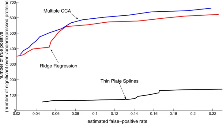
Validation of differential protein expression values In practical applications, the most important quality crite-rion for alignment methods of this kind is the number of proteins that are detected as significantly over-/underex-pressed. In order to estimate this number, all six experi-ments are pair-wise aligned and log-peptide abundance ratios are estimated for all jointly identified peptides. Equation 1 suggests to calculate the mean log-peptide abundance ratio averaged over all peptides which origi-nate from a particular protein. If this average log ratio deviates with t-test significance level αfrom zero then we declare this protein as strongly under- or overexpressed between the two conditions. The t-test with significance level αprovides us with a list of differently expressed pro-teins. This test can be applied to two samples measured (i) under different biological conditions or (ii) as technical
replicates. If the percentage of proteins detected as differ-entially abundant in different biological conditions pdiff
substantially exceeds the percentage of proteins detected as differentially abundant in replicates prep, then we can conclude that the difference in these biological conditions significantly influences the proteome. The reader should note that one should compare against biological repli-cates, to detect significant biomarkers. Unfortunately for our analysis, no biological replicates are available. But the technical replicates are still sufficient to show that the underlying method is able to detect differences in biolog-ical samples from different experimental conditions. A detection rate prep = αfor a t-test with significance level
α can be expected due to statistical fluctuations. We observed for our experiments that prep usually varies between 4% and 5% for α= 3% which is acceptable. The ratio prep/pdiff gives us now an estimate of the false discov-ery rate in the set of proteins detected as significantly dif-ferent abundant. Changes in the significance level α controls the false discovery rate. The number of true-pos-itive proteins are now estimated by the formula #posi-tive·(1 - false discovery rate).
Figure 3 shows the number of significantly different abun-dant proteins as a function of the false discovery rate. Mul-tiple CCA clearly outperforms ridge regression in the
Number of proteins classified as significantly over-/underexpressed as function of the estimated false discovery rate
Figure 3
Number of proteins classified as significantly over-/underexpressed as function of the estimated false discovery rate.
0.020 0.04 0.06 0.08 0.1 0.12 0.14 0.16 0.18 0.2 0.22 100 200 300 400 500 600 700
estimated false−positive rate
number of true positive
(number of significant over−/underexpressed protein
s)
Multiple CCA
Ridge Regression
number of estimated differential protein abundance lev-els at the same false discovery rate.
To compare the sensitivities of the alignment methods, we compare the number of differently abundant proteins detected by multiple CCA with the detections by ridge regression. The ratio of these two detection rates is shown as a function of the false discovery rate in Figure 4. The gain by multiple CCA is between 2% and 22% for differ-ent false discovery rates. The choice of a suitable false dis-covery rate depends on the proteomics application. In a biomarker discovery scenario we are interested in a fairly small false discovery rate to reduce the amount of work for experimental validation. In high throughput screening scenarios, bio-scientists are interested to find potential bio-markers that are further investigated by an additional sub-sequent analysis, and, therefore, they can accept more false discovery detections.
Conclusion
In this paper we are concerned with one of the critical steps in the data analysis of quantitative differential pro-teomics experiments. If an experiment with a liquid
chro-matography unit is repeated, one typically observes a non-linear deformation of the time scales.
A novel technique for aligning such time scales is pro-posed where the alignment method is based on general-ized canonical correlation analysis with a built-in non-negativity constraint. Two severe problems of previous approaches are solved with the novel technique: (i) non-symmetry of the time prediction function and (ii) a poten-tial violation of the monotonicity constraint which is inherent in temporal alignments. On a large proteomics dataset we demonstrate that jointly aligning multiply rep-licated experiments increases both precision and recall: the total number of peptide correspondences is increased as well as the quality of these matches is improved by the novel technique. These improvements directly influence estimates of differential protein expression values, because the number of proteins are significantly increased that are detected as differentially abundant in our experi-ments.
Ratio of the number of proteins classified as significantly over-/underexpressed as function of the estimated false discovery rate
Figure 4
Ratio of the number of proteins classified as significantly over-/underexpressed as function of the estimated false discovery rate. The ratio is between multiple CCA and pair-wise ridge regression.
0.021 0.04 0.06 0.08 0.1 0.12 0.14 0.16 0.18 0.2 0.22 1.05 1.1 1.15 1.2 1.25
estimated false−positive rate
gain of mCCA over ridge regression
Methods
Formal problem description
Assume we have to align K different time scales. Each time scale k is described by a list of peaks with time coordinates
Furthermore, a set of known correspondence points between time scales k and l
are provided by data base search. These time points are defined by those peptides that have been identified in both samples. For a peak p ∈ Pk we try to find a corre-sponding peak q ∈Pl (if there exists one), which formally
amounts to determine a mapping
fk,l : Pk →Pl ∪ {∅} (6) from the set of peaks Pk to the set of peaks Pl extended by the symbol ∅. This symbol ∅ represents the case that no corresponding peak can be found on the time scale l. Note that Eq. (6) defines a mapping between finite sets of time points.
To find a suitable mapping between the peaks, a continu-ous transformation between the time scales has to be learned. The function
gk,l : ⺢→⺢ (7)
transforms the (continuous) time scale k into the (contin-uous) time scale l. Given the time transformation gk,l we create the mapping fk,l as
The peak is mapped to the peak closest to the pre-dicted time on time scale l within a window of size w. The window size w controls the number of accepted corre-spondences. A smaller window size leads to a lower total number of accepted matches, but to a higher precision of the accepted correspondences, i.e. to an increased fraction of correct matches. A continuous time transformation gk,l
(see the next section for details) is learned and the trans-formation is evaluated using the mapping function fk,l.
Robust ridge regression
Fischer et al. [6] used robust ridge regression with polyno-mial basis functions to estimate the time transformation functions gk,l. Let be a tuple of
known time correspondences between time series k and l. The time is explicitly transformed to the polynomial basis . Without loss of generality it is assumed that the sample vectors φ(xi) have zero mean and unit covariance, otherwise the vectors are normalized accordingly. Robust ridge regression finds the parameter vector βthat minimizes
where L(ξ) is Huber's loss function [10]
However, the use of ridge regression to align time series has two disadvantages:
1. ridge regression is not symmetric in the sense that gl,k is
not an inverse of gk,l: x ≠gl,k(gk,l(x));
2. the time transformation function is not necessarily monotonically increasing. It might, thus, violate the monotonicity constraint that is inherent in temporal alignments.
Canonical correlation analysis
To overcome the above problems of ridge regression we propose to address the alignment task by way of canonical correlation analysis [11]. The two time scales are both mapped on a canonical time axis. Correlation analysis aims to find a linear projection on a canonical time axis such that the correlation between the two random varia-bles is maximized. Again we assume that the sample vec-tors φ(xi) have zero mean and unit covariance. The
objective is to find parameter vectors β1 and β2 that maxi-mize the correlation between the linear projections
φ(xi)tβ 1 and φ(xi)tβ2 Pk t k tnk k =
{
1}
( ) ( ) ,..., (4) Ck l, ={
(
t1( ) ( )k ,t1l)
,...,(
t( ) ( )mk,tml)
}
(5) fk l tjk t P dij i dij w dij ti l il l , ( ) ( ) arg min( ) { } :( )
= ∈ if where ∃ ≤ = −ggk l tj k , ( ) .( )
∅ ⎧ ⎨ ⎪ ⎩⎪ else (8) t( )jk ( , )x yi i =(
t( ) ( )ik ,til)
∈Ck l, φ( )xi =( , ,1x xi i2,...,xid t) Lc xi t yi t i n ( ( )φ β− )+λβ β, =∑
1 (9) L c c c c c c( ) , , . ξ ξ ξ ξ ξ = − > ≤ ⎧ ⎨ ⎪⎪ ⎩ ⎪ ⎪ 2 2 2 for for (10) maximize β φ φ β φ β φ β 1 2 1 1 2 1 2 2 t i i t i n i t i n i t i x y x y ( ) ( ) ( ( ) ) ( ( ) ) = = =∑
∑
11 n∑
(11)The denominator of Equation 11 can be reformulated as ||β1||·||β2||, since the covariance matrices and are normalized to unit covariance before. The problem can be solved directly by a transformation to the eigenvalue problem (see [12])
The vector β2 is then obtained by . In order to include the time-monotonicity constraint and robust-ness, however, it is advantageous to use an alternative for-malization of the optimization problem, which can be equivalently restated as follows (see [13]):
The function gk(xi) = φ(xi)tβk denotes the transformation
from the time scale k to the canonical time scale. Even for this reformulated problem, however, no guarantee is given that the transformation is monotonically increas-ing. In the case of a non-monotone function it is impossi-ble to find an unambiguous transformation between time scales k to l, because in general gk is not invertible. To overcome this problem we propose two changes in the setting of canonical correlation analysis:
1. A set of hyperbolic tangent basis functions is used. 2. A non-negativity constraint on the regression parame-ters is introduced.
The basis functions are defined as
The set of vectors z1,...,zd can either be chosen as the set of vectors x1,...,xn or as a set of d time points equally distrib-uted over the range of the respective time scale. The scal-ing parameter σcontrols the smoothness of the estimated alignment function.
If the parameters β1 and β2 are non-negative, the function
gk(xi) = φ(xi)tβ
k is monotonically increasing, because it is a
linear combination with non-negative coefficients of
monotonically increasing (hyperbolic tangent) functions. Instead of hyperbolic tangent functions, any other monot-onically increasing and bounded basis functions can be used. The alignment problem can now be defined as non-negative canonical correlation analysis with hyperbolic tangent basis functions. Learning the time warping requires to find the parameter vectors β1 and β2 that min-imize the objective function
We solve this problems iteratively by gradient descent. In a first step the objective function is minimized over β1 while keeping β2 fixed. Then the length of the vector β1 is normalized to fulfill the constraint ||β1|| = 1. In a second step the objective is minimized over β2 while keeping β1 fixed, and β2 is normalized accordingly. In each step of the iteration we have to solve a non-negative least-squares problem for which we use the Lawson-Hanson algorithm [14].
Using the above definition of the correlation problem we can easily extend the correlation coefficient to a robust ver-sion that is less sensitive to outliers. For that purpose the squared loss is replaced by Huber's robust loss function (Eq. 10)
Optimization of the robust CCA functional is similar to its quadratic counterpart (15), but with an additional inner loop that solves the robust non-negative least-squares problems by an iteratively re-weighted non-negative least-squares algorithm.
Multiple canonical correlation analysis
Sometimes there are only a very few peptides that are measured in both runs. In the case where one has more than two experiments one can benefit from multiple data-sets to increase the size of the training dataset. The prob-lem of canonical correlation analysis can be extended to multiple correlation analysis [15,16]. First notice that one can alternatively reformulate the two constraints ||β1|| = 1 and ||β2|| = 1 in Equation (13) to one single constraint ||β1|| + ||β2|| = 2 [17]. A possible extension of canonical correlation analysis to K time series is then defined by
Φ ΦX tX Φ ΦY Yt
λmax=sup{β1tΦ Φ Φ ΦX tY Y tXβ1| β =1} with Φx =( ( ),..., (φ x1 φxn)).
(12) β2 = Φ ΦY tXβ1 minimize ( ( )φ xi tβ φ( )yi tβ ) s t . . β , β . i n 1 2 2 1 1 1 2 1 − = = =
∑
(13) φ σ σ σ ( ) tanh( ( )) tanh( ( )) tanh( ( )) x x z x z x z i i i i d = − − − ⎛ ⎝ ⎜ ⎜ ⎜ ⎜⎜ ⎞ ⎠ 1 2 # ⎟⎟ ⎟ ⎟ ⎟⎟ . (14) minimize ( ( )φ xi tβ φ( )yi tβ ) s t . . β , β ,β , . i n k j 1 22 1 1 1 2 1 0 − = = ≥ =∑
(15) minimize Lc xit yit s t i n k j ( ( )φ β1 φ( )β2) . . β , β ,β , . 1 1 1 2 1 0 − = = ≥ =∑
(16) minimize Lc tik t k til t l s t i m k l K k k l ( (( )) (( )) ) . . , φ β −φ β β = ≤ < ≤∑
∑
1 1 == ≥∑
K,βk j, 0. k K =1 (17)This problem is again solved iteratively by minimizing the objective function with respect to one vector βk while keeping the other vectors βl, l ≠k fixed. The pseudo code is given in Figure 5.
Competing interests
The authors declare that they have no competing interests.
Authors' contributions
All authors developed the methods, designed and per-formed comparisons of methods, and wrote the manu-script.
Acknowledgements
The authors like to thank J. Grossmann, S. Baginsky and W. Gruissem for valuable discussions and the competence center of systems physiology and metabolic diseases (ETH Zurich), for support.
This article has been published as part of BMC Bioinformatics Volume 8 Sup-plement 10, 2007: Neural Information Processing Systems (NIPS) work-shop on New Problems and Methods in Computational Biology. The full contents of the supplement are available online at http://www.biomedcen tral.com/1471-2105/8?issue=S10.
References
1. Nielsen NPV, Carstensen JM, Smedsgaard J: Aligning of single and multiple wavelength chromatographic profiles for
chemo-Pseudo-Code for non-negative CCA algorithm
Figure 5
Pseudo-Code for non-negative CCA algorithm.
NN-CCA(
C
·,·)
//
Let
t
kidenote the current estimate of the canonical time.
//
Initialization. Set the current estimate of canonical time of the first time axis to the given time.
∀
i
:
t
(1)i=
t
(1)ifor
k
= 2
to
N
//
centralize to zero mean and unit covariance
centralize
φ(t
ki
)
//
non-neg. least squares regression against the estimated canonical time points of the time axis
l < k
.
β
k←
NNLS
t
i(k),
t
i(l)∈
C
k,l, l < k
//
Prediction of the canonical time of points on axis
k
∀
i
:
t
(ik)←
φ(t
k i)
tβ
kendfor
//
Iteration.
for
i
= 1
to
nrOfIterations
for
k
= 1
to
N
//
centralize to zero mean and unit covariance
centralize
φ(t
ki
)
//
non-neg. reg. against the estimated canonical time points of the other time axis
l
=
k
.
β
k←
NNLS
t
i(k),
t
i(l)∈
C
k,l, l
=
k
endfor
//
Normalization
s
←
1≤k≤Nβ
k∀
1
≤
k
≤
N
:
β
k←
1sβ
kfor
k
= 1
to
N
//
Prediction of the canonical time of points on axis
k
∀
i
:
t
(ik)←
φ(t
k i)
tβ
kendfor
endfor
Publish with BioMed Central and every scientist can read your work free of charge
"BioMed Central will be the most significant development for disseminating the results of biomedical researc h in our lifetime."
Sir Paul Nurse, Cancer Research UK
Your research papers will be:
available free of charge to the entire biomedical community peer reviewed and published immediately upon acceptance cited in PubMed and archived on PubMed Central yours — you keep the copyright
Submit your manuscript here:
http://www.biomedcentral.com/info/publishing_adv.asp
BioMedcentral metric data analysis using correlation optimised warping. J
of Chromatography A 1998, 805:17-35.
2. Listgarten J, Neal RM, Roweis ST, Emili A: Multiple alignment of continuous time series. Neural Information Processing Systems 2005, 17:817-824.
3. Listgarten J, Neal RM, Roweis ST, Wong P, Emili A: Difference detection in LC-MS data for protein biomarker discovery.
Bioinformatics 2007, 23:e198-1204.
4. Tibshirani R, Hastie T, Narasimhan B, Soltys S, Shi G, Koong A, Le QT: Sample classification from protein mass spectrometry, by peak probability contrasts. Bioinformatics 2004, 20:3034-3044. 5. Kirchner M, Saussen B, Steen H, Steen JA, Hamprecht FA: amsrpm: robust point matching for retention time alignment of LC/ MS data with R. Journal of Statistical Software 2007, 18:.
6. Fischer B, Grossmann J, Roth V, Baginsky S, Gruissem W, Buhmann JM: Semi-supervised LC/MS alignment for differential pro-teomics. Bioinformatics 2006, 22(14):e132-e140.
7. Tang H, Arnold RJ, Alves P, Xun Z, Clemmer DE, Novotny MV, Reilly JP, Radivojac P: A computational approach toward label-free protein quantification using predicted peptide detectability.
Bioinformatics 2006, 22(14):e481-e488.
8. Aebersold R, Mann M: Mass spectrometry-based proteomics.
Nature 2003, 422:198-207.
9. Sadygov RG, Cociorva D, JRY III: Large-scale database searching using tandem mass spectra: looking up the answer in the back of the book. Nature Methods 2004, 1(3):195-202.
10. Huber P: Robust statisticsNew York: Wiley; 1981.
11. Hotelling H: Relations between two sets of variates. Biometrica
1936, 28:321-377.
12. Hardoon DR, Szedmak S, Shawe-Taylor J: Canonical correlation analysis: an overview with application to learning methods.
Neural Computation 2004, 16:2639-2664.
13. Kuss M, Graepel T: The geometry of kernel canonical correla-tion analysis. In Tech Rep TR-108Max Planck Institute for Biological Cybernetics, Tübingen, Germany; 2003.
14. Lawson CL, Hanson RJ: Solving least square problemsVolume chap 23.
Prentice Hall; 1974.
15. Yamanishi Y, Vert JP, Nakaya A, Kanehisa M: Extraction of corre-lated gene clusters from multiple genomic data by general-ized kernel canonical correlation analysis. Bioinformatics 2003, 9(Suppl 1):i323-i330.
16. Bach FR, Jordan MI: Kernel independent component analysis.
Journal of Machine Learning Research 2002, 3:1-48.
17. Via J, Santamaria I, Perez J: Canonical correlation analysis (CCA) algorithms for multiple data sets: application to blind simo equalization. European Signal Processing Conference 2005.