Adaptive Non-negative Least Squares with Applications
to Non-Negative Matrix Factorization
A THESIS
SUBMITTED TO THE FACULTY OF THE GRADUATE SCHOOL OF THE UNIVERSITY OF MINNESOTA
BY
Artem Mosesov
IN PARTIAL FULFILLMENT OF THE REQUIREMENTS FOR THE DEGREE OF
MASTER OF SCIENCE
Nikolaos Sidiropoulos
c
Artem Mosesov 2014 ALL RIGHTS RESERVED
Acknowledgements
First and foremost, I would like to thank my advisor, Professor Nikoloas Sidiropoulos. I am grateful not only for his help and guidance, but also for the endless patience he demonstrated throughout the course of my graduate work. This would not have been possible without his help, and I’ve always felt privileged to be one of his students.
I would also like to thank the fellow students in my group, along with all the students, researchers, and visitors, in the department. I have spent many hours in this company, and feel that my time spent here would not have been the same without them. I’ve enjoyed many academic and non-academic digressions in this group.
Finally, I would like to thank my parents, Oleg and Diana. Their continual support and encouragement has been a blessing during my graduate work, and their help extends far beyond this scope. I am thankful for the virtues they never ceased to instill in me.
Abstract
Problems with non-negativity constrains have recently attracted a great deal of interest. Non-negativity constraints arise naturally in many applications, and are often necessary for proper interpretation. Furthermore, these constrains provide an intrinsic sparsity that may be of value in certain situations. Two common problems that have gathered notable attention are the negative least squares (NNLS) problem, and the non-negative matrix factorization (NMF) problem. In this paper, a method to solve the NNLS problem in an adaptive way is discussed. Additionally, possible ways to apply this, and other related method, to adaptive NMF problems are discussed.
Contents
Acknowledgements i Abstract ii List of Figures v 1 Introduction 1 2 Offline/Batch NNLS 3 2.1 Speed Improvements . . . 6 3 Adaptive NNLS 8 4 Implementation 14 4.1 Set Pivoting . . . 144.2 Numerical Stability of pseudo-inverse updates . . . 17
4.3 Cholesky Updates . . . 17 5 NMF 19 5.1 Supervised Online NMF . . . 21 5.2 Semi-Supervised Adaptive NMF . . . 23 5.3 Complete Adaptive NMF . . . 25 6 Results 26 6.1 NNLS . . . 26 6.2 NMF . . . 29 iii
7 Conclusion 35
References 36
List of Figures
3.1 Example of the process required to update the NNLS solution with a
single addition of data. . . 11
6.1 Number of inner-iterations required by FNNLSb vs. SPP per
outer-iteration. Initial data size is 1000x100. . . 26
6.2 Cumulative run-time of FNNLSb vs. SPP corresponding to the
simula-tion in Figure 6.1. Initial data size is 1000x100. . . 27
6.3 AdBPP compared with warm started BPP. AdSPP also included for
ref-erence. Initial data size is 15,000x500. FinalNP = 176. Average change
in passive set size per iteration is 1.37, with maximum change being 6. . 28
6.4 AdBPP compared with warm started BPP. Initial data size is 50,000x300.
FinalNP = 219. Average change in passive set size per iteration is 0.24,
with maximum change being 2. . . 28
6.5 AdBPP compared with warm started BPP. Initial data size is 500x100.
FinalNP = 43. Average change in passive set size per iteration is 1.57,
with maximum change being 5. . . 29
6.6 Improvement of AdBPP over PBPP is compared for various data sizes. . 29
6.7 Comparison of online semi-supervised NMF using AdBPP-SSNMF, MU,
ALS. Initial data size is M = 80, R = 50, N = 100. . . 31
6.8 Comparison of supervised, semi-supervised, and full NMF methods for
updating NMF factors. . . 32
6.9 Comparison of singly iterated warm started ANLS-BPP, HALS, and
HALS-BPP. Initial data size is M = 100, R = 30, N = 200. . . 33
6.10 Comparison of singly iterated warm started ANLS-BPP, HALS, and full
ANLS-BPP for MovieLens data. . . 34
Chapter 1
Introduction
The non-negative least squares (NNLS) problem has been of considerable interest for many years, and continues to find many applications in problems where non-negativity constraints play an important role. NNLS has various applications, including chemo-metrics , signal processing, and machine learning. It has also seen success in image deconvolution for teloscopy as well as mass spectrography in bioinformatics [1, 2, 3]. Moreover, methods for solving the NNLS problem have been successfully used for NMF,
and even non-negative tensor factorization (NTF) by an alternating non-negative least
squares (ANLS) approach [4, 5, 6]. With rising interest in non-negativity constraints, efficient methods for NNLS deserve attention.
Typically, most of these applications use NNLS to analyze data offline. While this is often suitable for most applications, many other algorithms have benefited greatly from modifications to allow for quick updating (the unconstrained least squares (LS) being a good example.) This may be done for the goal of having a real-time system, or simply for updating models for very large data sets in an efficient way. With non-negatively constrained problems showing up in more and more applications, updative methods for these problems appear very attractive. In this paper, we explore a low complexity method for solving the NNLS problem adaptively. Furthermore, we consider ways to apply this method to various versions of adaptive NMF problems.
We first look at two common algorithms for the NNLS problem - fast non-negative least
2 squares (FNNLS), and block-principal-pivoting (BPP). By slightly modifying a strategy used by FNNLS and providing efficient updates to the solution, we come up with an algorithm termed AdSPP. This proves to be faster for adaptive settings than FNNLS, but typically slower than BPP (in the vast majority of cases). Adding efficient updates to BPP in a similar way, we show that the resulting algorithm (termed AdBPP) is a more efficient way to compute a slowly changing NNLS problem. Later in the paper, we suggest a possible way to update the NMF solution online using AdBPP, terming the algorithm AdBPP-SSNMF.
Chapter 2
Offline/Batch NNLS
NNLS is a quadratic programming problem, and can be optimally solved with various
methods, including projected gradient descent and interior point methods. Thede facto
method for NNLS has been theactive set method proposed by Lawson and Hanson [7]. A
computationally less expensive version of this algorithm was discussed and implemented by Bro [6]. This has been a staple algorithm for providing an efficient NNLS solution. A
similar, but more generalized, block principal pivoting algorithm has also been analyzed
by Portugal [8], and later revisited by Kim and Park [5] for NMF applications. The latter method has been shown to be the most computationally efficient for NNLS. While the above methods achieve optimal solutions to the NNLS problem, they become difficult to scale to very large problems due to the required computational complexity and slow convergence rates. Furthermore, since they have been developed for offline settings, these algorithms may not be ideal for adaptive applications, as they do not fully exploit the slowly changing structure of the problem. In the following, we explore a possible method for adaptive NNLS. That is, given a current solution to the NNLS problem, attempt to efficiently update the NNLS solution as data is accessed sequen-tially. Since the proposed approach is a modification/extension of the aforementioned algorithms, we briefly discuss them here.
4 The general NNLS problem is formulated as follows:
min
x≥0kAx−bk 2
2 (2.1)
The Lagrangian is then
kAx−bk2
2+λTx (2.2)
where λ is the Lagrange multiplier. For an optimal solution x, we have the
Karush-Kuhn-Tucker (KKT) conditions as follows
λ=AT(b−Ax)
λixi = 0, ∀i
λ≤0
(2.3)
The first expression follows from the necessary condition that the derivative of the dual
variable with respect toxis zero. From these conditions we get the following properties
for the solution xand the corresponding Lagrange multipliers λ
xi >0, λi = 0, ∀ i P
xi = 0, λi <0, ∀ i E
(2.4)
whereP is the passive (index) set of the solution, and E is the active (index) set of the
solution.
The active-set and the block pivoting method both use the KKT conditions, and the
fact that knowing (a priori) the passive set, one can determine the optimal solution by
simply solving an unconstrained least squares problem on this set. That is, given the
passive set P, the optimal solution to (2.1) can determined as follows
xP = [ATPAP]−1ATPb
xE =0
5
where xP and xE refer to the active and passive portions of the solution, respectively.
AP is a matrix composed of the columns of A corresponding to the passive set. (The
same notation will freely be used in the rest of the text in reference to other vari-ables.)
The block pivoting algorithm relies on alternately solving for xP via (2.5), and λE via
(2.3), and updating the passive and active set according to (2.4). That is, any negative
xP and positiveλE values are set to 0, and the respective indices reassigned to the active
or passive set. The active-set algorithm operates in a similar fashion, but exchanges only one component at a time. Both of these algorithms have been shown to converge to the correct set partition in a finite number of iterations [7, 8, 5]. There are two main differences between these two methods that are worth noting. The block pivoting algorithm allows for exchanging multiple components at once. This facilitates faster convergence, especially when dealing with large regression vectors. The other main difference is that the active-set algorithm retains feasibility of the solution throughout the procedure. That is, after transferring a component into the passive set and solving unconstrained least squares on that set, a line search is performed to bring the solution back to the feasibility region. In this way, components are taken back out of the passive set in a different way than the block pivoting method. A more detailed survey of these algorithms, along with various heuristics, can be found in [7, 8, 6, 5].
Before continuing, we quickly mention that the update in (2.3) may equivalently be performed as follows,
λE =ATE(b−APxP)
λP = 0
(2.6)
6
2.1
Speed Improvements
A significant speed improvement to the active-set algorithm has been suggested and
implemented by Bro in [6], termedfast non-negative least squares (FNNLS). This
mod-ification provides a way to reduce the computational load caused by matrix-matrix multiplications. Recalling that the passive set is updated at each iteration, an update
of xP via (2.5) requires the matrix-matrix productATPAP.
FNNLS takes advantage of the fact that the matrixATPAP can actually be constructed
from elements of ATA. Specifically, given B:=ATA,ATPAP is composed of elements
Bij, i, j P. Recognizing this allows us to do a single matrix-matrix computation,
ATA, at the start of the algorithm, and obtain AT
PAP at each iteration by simply
taking elements of the precomputed matrix. In the same way, we may precomputeATb,
and use this to avoid computing ATPb. These computational savings easily extend to
the Lagrange update when we rewrite (2.3) as λ = ATb−ATAx. This, of course,
requires extra storage of the matrix ATA; nevertheless, this memory-speed trade-off
is often welcomed. Furthermore, in a highly overdetermined setting (M N), this
requirement is not as restrictive as storing the entire matrix A, which may be less
feasible for very large problems.
Before continuing, it may be appropriate to consider the computational advantages of FNNLS in the light of current approaches to LS. We described the efficiency of FNNLS as was done in [6, 5], that is, stemming from avoiding matrix-matrix computations. Although the update for the active set algorithm was originally presented as (2.5), this is seldom done to compute the LS solution. Instead, more computationally efficient and numerically stable methods (e.g., Gaussian elimination) are frequently used (for example, the MATLAB ’mldivide’ operator.) With this noted, it seems more insightful to point out that the effective benefit of FNNLS is from forming the normal equations
ATAx=ATband recognizing that the normal equations on the passive set are simply
a subset of these. The computational advantages, then, are only applicable for over-determined systems (which is the case for the PARAFAC problem considered in [6]).
Without utilizing the normal equations, the original active set algorithm has O(M N2)
7
O(M N2), followed byO(N3) complexity in each iteration. One may recognize that the
use of the normal equations comes at the price of numerical stability. This approach, therefore, may not be appropriate when presented with an ill-conditioned problem. Since well-conditioned data is commonly assumed, we shall also retain this assumption.
Chapter 3
Adaptive NNLS
As in the standard adaptive LS setting, we consider updating the current NNLS solution
online, as additional data is acquired sequentially. That is, given a solution to
min
x0≥0
kA0x0−b0k22 (3.1)
we would like a fast update to solve (2.1), with
A= " A0 aT1 # and b= " b0 b1 # (3.2)
whereaT1 and b1 are new row and scalar additions toAandb, respectively. We consider
the problem in a typical, overdetermined system. That is, A∈RM×N, M > N.
In the unconstrained case, this problem is readily addressed using the recursive least
squares (RLS) algorithm. This method utilizes the matrix inversion lemma to provide
computationally cheap updates to the pseudo-inverse of A. We attempt to approach
the adaptive NNLS problem in a similar spirit.
As new data is acquired, the well-developed techniques for the RLS problem may simply be used to update the unconstrained LS solution on the passive set. However, since the
9 data is now changed, the non-negativity must be accounted for once more. Naively, this requires a call to a NNLS-solving routine, such as FNNLS, which would then solve the problem in a ’batch-like’ manner. So, merely using RLS on the unconstrained problem does not facilitate a fully adaptive, nor recursive, method of NNLS. The non-negativity of the components of the solution (in other words, the active and passive sets) needs to be efficiently tracked as well.
We may use to our advantage the following observation. Given a good solution to the current problem, the solution to the next problem will not change by much (naturally, this isn’t very surprising, and is commonly noted for unconstrained LS.) Hence, we may claim that changes to the passive set are also minimal. This, in fact, was also noted in [6] (in the case of PARAFAC loadings). Realizing this allows a warm start of FNNLS, which significantly reduces the number of iterations required to converge. (In the case of no change in passive set, the solution is achieved by effectively solving a single unconstrained LS problem.) In [6], warm starting FNNLS (termed FNNLSb) provides a relatively quick way to compute the NNLS solution.
It is important to realize here that while FNNLSb improves computation time through
the way it acquires ATPAP, it still suffers from O(N3) complexity involved in solving
LS problems for determining changes in the passive/active sets. Utilizing the passive set from the previous solution is readily exploited for initialization, but not for the computations that follow. We may, however, note that if the passive set does not change
by much, then xP at each new iteration is simply the old xP with few elements added
or removed (according to the change in setP.) Since we are concerned with solutions to
APxP =b, a method for updatingxP without re-solving a least squares problem would
be very beneficial. Not surprisingly though, this problem has been addressed before. In fact, recomputing the pseudo-inverse of a matrix under a column addition or removal can be done in a similar fashion as under a row addition. This typoe of update has been discussed in [9, 10]; we briefly mention the results.
Let us consider an addition or removal of a single column. The following observations
are the key to avoidingO(N3) complexity associated with re-solving least squares
prob-lems upon changes to passive set. (The first two lemmas may be observed from the block matrix inversion. The third arises simply from basic properties of permutation
10 matrices.)
Lemma 1 - Inverse of positive definite matrix under column addition:
Given an inverse P = [ATA]−1, we can determine the new inverse Pn = [ATnAn]−1,
where An= [A v]contains a new column v, as
Pn= " H g gT z # , where z = 1 vTv−wTPw g=−Pwz H=P+ Pww TP vTv−wTPw with w:=ATv
Lemma 2 - Inverse of positive definite matrix under column removal:
Given an inverse Pn= [ATnAn]−1 , we can determine the new inverse P= [ATA]−1 as
P=H−gg
T z
where H, g, and z, are blocks of Pn, as before.
Lemma 3 - Permutation within inverse
Denoting P := [ATA]−1 for some matrix A, as before, we consider permuting the columns of A to get B := AΠ (where Π is a permutation matrix functioning on the columns of A). Then
PB:= [BTB]−1 =ΠT[ATA]Π
The first two observations allow the pseudo-inverse of AP to be efficiently updated
11 allows us to extend these results to a column addition/removal anywhere in the matrix. This is similar to the way RLS employs the matrix inversion lemma to recompute the pseudo-inverse upon a row addition.
We note that in the setting here, an added column is never arbitrary, and is always
a column of A. If we keep ATA in memory, as done in FNNLS, ATv need not be
computed (which would result in O(M N) complexity), and can simply be taken as one
of the columns of ATA. This allows the update to retain O(N2) complexity, as in the
standard RLS update for unconstrained LS. Recall that new data still comes as new
rows aTk inA, and scalars bk inb. This does not pose a problem in needing ATA and
ATb, as these may easily be updated as follows.
ATA←ATA+akaTk
ATb←ATb+bkak
(3.3)
We now briefly summarize the mains steps required in updating the NNLS solution as
discussed above. Upon arrival of new data, we update ATA and ATb, along with the
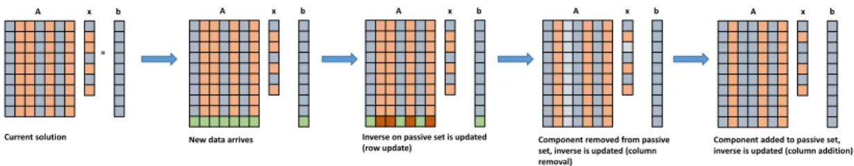
unconstrained solution on the passive set using well known RLS methods. This is done once for each new data element that arrives. After this is done, we use the method of FNNLS/single-pivoting combined with Lemmas 1-3 to adjust for any changes in the passive/active sets, and compute the final solution. This may take a number of iterations, depending on how much the passive set changes (or none, if the set remains the same.) Figure 3.1 demonstrates this process.
A x b
=
A x b A x b A x b A x b
Current solution New data arrives Inverse on passive set is updated
(row update) Component removed from passive set, inverse is updated (column removal)
Component added to passive set, inverse is updated (column addition)
Figure 3.1: Example of the process required to update the NNLS solution with a single addition of data.
12 Adjusting the passive set efficiently is key to attaining fast updates for the NNLS
so-lution. To avoid confusion, we may refer to the first stage as outer-updates/iterations,
and the second stage as inner-updates/iterations. These stages correspond to
updat-ing the inverse of ATPAP upon row addition to AP (rank-1 addition to ATPAP), and
column addition/removal to AP (corresponding to row and column addition/removal
of ATPAP), respectively. Since the focus here is on the inner-updates, we avoid avid
discussion of the outer-updates, as this is a problem that has been studied extensively for unconstrained LS updates. We may also recognize that the worst case complexity
has been quoted, thus far, in terms ofN. However, denoting the number of components
in the passive and active sets asNP and NE, respectively, we provide the order of
com-putational complexity per iteration/component-exchange (ignoring the outer-updates) for the active set method, standard FNNLS, and the method proposed (which we term AdFNNLS) here below.
Active-set: O(M NP2 +NENP)
FNNLS: O(NP3 +NENP)
AdFNNLS: O(NP2 +NENP)
The first term comes from solving the unconstrained least squares problem on the
pas-sive set, and the second term comes from updating the dual variable. (The block
pivoting algorithm has the same complexity per iteration as FNNLS.) This allows us to recognize the following: if the passive set is significantly smaller than the active set, the computational benefits from the updates are marginal, since the update of the duel variable will dominate the computation. Hence, we note that the method discussed here is only applicable when the passive sets are reasonably large. One may conclude
that this method becomes favorable roughly when NP2 > NE. Although most
inter-esting problems requiring NNLS have a non-dense solution, the condition above is not particularly restrictive when dealing with reasonable data sizes.
Efficiently updating the NNLS solution upon column exchanges has in fact been orig-inally mentioned in [8] with respect to block pivoting. It was not recommended as an effective way to speed up computations in general; this is due to the multiple (possibly many) exchanges that happen in each iteration of the block pivoting algorithm. While
13 the idea still applies to the active-set algorithm, the approach becomes somewhat coun-terproductive in the batch method, as the active-set algorithm doesn’t reap the fast convergence benefits of block pivoting. The same idea has also been explored in [11] for solving many NNLS problems using GPUs and a parallelized approach. The method there was admittedly not scalable to large problems, and furthermore, abandons the fast convergence rate of block pivoting for the single pivots of the active-set algorithm. We remark that the motivation in this paper is to provide relatively fast updates suitable foradaptive methods, as opposed to providing a fast batch algorithm.
Chapter 4
Implementation
4.1
Set Pivoting
Thus far, we recognize that, when given a non-negative solution to the NNLS problem, an updated solution upon new data arrival will not change significantly. With this, the exchange of indices between the passive and active sets is expected to be minimal. Realizing this, we can update the solution efficiently upon the set-exchange of a single component (that is, moving it from active to passive, or vise verse), we may opt to
implement the single principle pivoting algorithm (in which only one component is
exchanged between sets in each iteration.) This is reasonable, since minimal exchanges are expected.
In [5], the active-set algorithm is described as an instance of a single pivoting algorithm. Indeed, this is one way single pivoting may be realized. We emphasize a small difference in way we carry out the set exchanges. The active-set algorithm contains a main while-loop, in which components are moved into the passive set, and an inner while-while-loop, in which the components are moved out of the passive set. This works well when initializing with an empty passive set. In this setting, the algorithm seldom enters the inner loop, and spends most of the time putting elements into the passive set. Upon running into an infeasible solution, the inner loop removes the components out of the feasible set until feasibility is achieved. Furthermore, a line-search adjustment is made to the entire
15 solution vector to restore feasibility. The FNNLS algorithm retains the same approach. If we initialize with the previous solution, however, there should be no expectation (unless otherwise domain-related) as to how many elements leave or enter the passive set). With this noted, we find it more suitable to implement the exchanges equally. That is, we take turns between bringing single elements into and out of the sets. This style of exchange more closely resembles the general approach for block pivoting discussed in [5], but with single pivots. The rules we use for exchanging components between the sets are as follows. For placing an infeasible (negative) regression component into the active set, we pick the index corresponding to the smallest negative regressor value. This value is then simply zeroed out. The passive components are not changed, unlike they are in the line-search adjustment. For transferring components into the passive set, we pick the index corresponding to the largest (positive) of the Lagrange multipliers (exactly as in the active-set method/FNNLS.) Although this is a rather trivial adjustment to how the exchanges are performed in FNNLS, our experiments show that this typically results in significantly fewer iterations in updating the solution.
While this form of single principal pivoting is later shown to be more appropriate for adaptive NNLS than the active-set algorithm, it is a rather conservative approach. That is, only a single exchange is made between the sets before checking the optimality con-ditions. This is done under the assumption of minimal set changes, in hopes to prevent unnecessary exchanges that can be made using the full block pivot. Experiments show, however, that the majority of the time, doing a full block pivot will only take a single it-eration without requiring another one for correction. Noting this, we find it more appro-priate to use the full block exchanges of BPP. The inverse/Cholesky updates/downdates may then be done sequentially (or in block form, if multiple neighboring components are exchanged).
We term the adaptive single principal pivoting and block principal pivoting algorithms as AdSPP and AdBPP, respectively. The pseudo-code for both of these is presented below.
16
Algorithm 1 - AdSPP
Require: xk−1, [ATk−1Ak−1], [ATk−1bk−1], [ATk−1Ak−1]−P1
Input: New data ak,bk
Update normal equations according to 3.3
Update [ATk−1Ak−1]−P1 and xP =kAPxP −bk22 using RLS with new dataakP,bk
if any xi <0 thenmove indexj = arg min
i
(x) out of P
λE =ATE(b−APxP) , λE =0
if any λj >0then move indexj= arg max
i
(λ) into P
whilenot optimal (according to (2.3))
Solve xP =kAPxP −bk22 by updating [ATk−1Ak−1]−1 using Lemmas 1-3.
if anyxi<0then move indexj= arg min
i
(x) out of P
λE =ATE(b−APxP) λE =0
if anyλj >0 thenmove index j= arg max
i
(λ) into P
Algorithm 2 - AdBPP
Require: xk−1, [ATk−1Ak−1], [ATk−1bk−1], [ATk−1Ak−1]−1 Input: New data ak,bk
Update normal equations (according to 3.3)
Update [ATk−1Ak−1]−P1 and xP =kAPxP −bk22 using RLS with new dataakP,bk
λE =ATE(b−APxP) , λE =0
Update P and E sets according to (2.4) with full exchange rule
whilenot optimal (according to (2.3))
UpdatexP =kAPxP −bk22 using Lemmas 1-3.
λE =ATE(b−APxP) λE =0
17
4.2
Numerical Stability of pseudo-inverse updates
The RLS algorithm is a well known method that has been subject to a long list of variations, and has been applied in numerous applications. Unfortunately, the RLS method is also known to suffer from numerical instability under finite-point arithmetic. This originates from the use of the matrix inversion lemma for updating the matrix inverse. While this has been mitigated in much of the signal processing domain through various means, most of those efforts can not be extended here due to a lack of shifting
structure in the matrix A and the submatrixAP. Furthermore, we can not rely on a
forgetting factor to prevent the accumulation of error when updating the pseudo-inverse for column exchanges. Upon further inspection, however, the situation here does not appear detrimental.
Recall the use of the matrix inversion lemma applied to the column update,
H=P+ Pww
TP
vTv−wTPw
This equation corresponds to a rank-1 downdate of the pseudo-inverse. A catastrophic
error may occur when the denominator is very close to zero; that is, whenwTPw≈vTv.
This occurrence becomes more clear when we rewrite,wTPw=vTA[ATA]−1ATv. We
see then, that the denominator is exactly zero when the newly added columnvis already
contained in A. More generally, the denominator takes on a very small value when a
column added is highly correlated to an existing one. However, the columns that we are
adding (and removing) are not random; they are simply the columns of A. Hence, if a
well-conditioned system is assumed, this cancellation does not become a concern.
4.3
Cholesky Updates
Although in many cases we may be satisfied using the above updates, certain situations may render the RLS-style inversion impractical. Even if the non-ideal numerical prop-erties of the matrix inversion lemma are acceptable, it’s worthwhile to recognize that when encountering large, sparse matrices, the pseudo-inverse tends be dense.
18 In [11], the QR decomposition was used for this intent. While the QR decomposition is
preferred for its numerical stability, the orthogonal matrix Q tends to be dense.
Fur-thermore, this matrix is large, and its computation results in decreased computational speed.
In order to avoid storing and computing the Q matrix, we consider the Cholesky
de-composition ofATA. We remark that this closely resembles the semi-normal equations
discussed in [12], shown below.
RTRx=ATb
Instead of using the R from the QR decomposition, we may use R from the Cholesky
decomposition. This will retain the stability of the normal equations while avoiding
the Q matrix altogether. The stability of this is studied in [12, 13]. Rank-1 and
row/column updates and downdates to the Cholesky factors have been studied and revisited in numerous papers, including [14, 15, 16, 17].
The updates and downdates to the Cholesky factor can be accomplished using backsolve
routines and Jacobi/Givens rotations to achieve a computational complexity of O(N2)
(per row or column update). We refer the reader to the previously referenced papers for the details, and end this section noting that these types of updates (whether QR or Cholesky) have been explored before in various applications and even optimized for various system structures, including VLSI, FPGA, systolic array, and pipelined implementations.
Chapter 5
NMF
Ever since the initial research by Paatero [18] and Lee [19], NMF has received great attention. Numerous methods and variations of NMF algorithms have been proposed and explored in applications including spectral separation, text data mining, image analysis, clustering, and bioinformatics [4].
The NMF problem is formulated as follows
min
W,H≥0kY−WHk 2
F (5.1)
with Y∈RM×N,W∈RM×R,H∈RR×N.
We briefly mention the most commonly used techniques for solving this problem. The
most common approach is to alternately solve for W and H (typically referred to as
block coordinate descent). Since NMF is a non-convex problem, this approach is taken
with the goal of reaching a local minimum. If W and H are updated using locally
optimal updates, the block coordinate descent has been proven to converge to a local stationary point.
This problem has commonly been approached by using the alternating least squares
(ALS) method. This algorithm alternates between solving for W and H by using
unconstrained LS followed by a projection onto the non-negative orthant (nulling out
20 any negative values). Although this algorithm is fast, it updates each matrix using a non-optimal technique, and hence, is not guaranteed to converge. Because of this, the ALS method often leads to a poor solution.
The other workhorse in NMF is the method of multiplicative updates (MU) proposed in [19]. This method uses non-increasing updates to do block coordinate descent. The multiplicative nature of the updates assures that non-negative values do not change sign. While this algorithm achieves a better solution, it tends to exhibit slow convergence in practice [20].
Recently, more robust and efficient techniques have been developed for the NMF
prob-lem. Two state of the art techniques that have seen great success are the hierarchical
alternating least squares (HALS) [4] and alternating non-negative least squares with
BPP ANLS-BPP [5]. Both of these techniques solve the respective constrained least
squares problems optimally, and hence, posses convergence properties necessary for a
block coordinate descent scheme. HALS does this by solving for columns of W and
rows of H while fixing the rest of the data. ANLS-PP, on the other hand, uses the
BPP technique developed for non-negative least squares to solve for rows of W and
columns of H. Moreover, both of these techniques have been shown to not only
outper-form the ALS and MU methods, but also be capable of approaching the newly derived Cramer Rao bounds for unique NMF decompositions (under certain conditions) [21]. This makes HALS and ANLS-BPP particularly desirable for applications where inter-pretability is sought. In general, HALS has less computationally expensive updates, but may require more iterations to converge. HALS is typically the more efficient algorithm for dense matrices, whereas ANLS-BPP tends to be more efficient with sparse matrices [5]. (As seen earlier, this partly stems from the fact that the cost of BPP relies on the support/passive-set of the solution.)
Recognizing that ANLS-BPP is a good method for NMF, we may consider using the method of adaptive NNLS developed earlier for adaptive NMF. Adaptive NMF has been studied in various settings and contexts before; we consider the setting commonly used (though, not limited) in spectral separation applications. In this context, we attempt
to separate or decompose a spectral mixture. The observation matrix Y denotes the
21
time i. W and Hare the factors, with W typically being referred to as thedictionary
(that is, each columnwi corresponds to the spectrum of thei’th signal in the mixture)
and His referred to as the activation matrix (that is, each column hi describes which
signals are present at some time instance k). Treating this problem in an adaptive
fashion, we effectively want to perform spectral factor analysis online. Let us first
formulate this problem as
min Wk,Hk≥0 kYk−WkHkk2F (5.2) whereYk= h Yk−1 yk i
contains the old dataYk−1, and a new data frameyk acquired
at time instance k. As before, we assume that the previous factors Wk−1 and Hk−1
are known, and we (most generally) want to efficiently update these factors to Wk and
Hk.
This problem has been considered in [22, 23, 24]. In [22] and [23], this was accomplished by using MU. In [24], this was accomplished by using the ALS-like approach (in which the unconstrained LS solution is projected to the non-negative orthant) combined with speed benefits from using the matrix inversion lemma. Although efficient, the MU and projected LS methods have been shown to be less than ideal for NMF. We may then seek to use better methods, while retaining the approximate computational complexity of the algorithm. In this way, the quality of the solution is not reduced for speed. Let us look at some situation-specific settings used in this context.
5.1
Supervised Online NMF
We first consider the case of supervised online NMF as described in [23, 22]. In this
setting, it is assumed that we already know the dictionary W (so, perhaps we know all
the spectral characteristics of each source, and simply want to separate them.) So, at
22 in a NNLS problem at each time frame
min
hk≥0
kyk−Whkk2F (5.3)
To solve this, we may then simply use the block pivoting method instead of projected least squares method (which is highly suboptimal) or the MU scheme (which tends to have very slow convergence and requires many iterations). This will guarantee an
opti-mal solution. Computing the new frame from scratch will then requireO(R3) complexity
per iteration. In order to utilize the adaptive method discussed for NNLS, though, we rely on new data only slightly changing the solution. While this doesn’t come as natu-rally to the formulation presented here, it may be a safe assumption depending on the context. Consider an example of speech separation applications (often referred to as the ’cocktail party’ problem). In this problem, we attempt to separate the sources of speech from the acquired spectral mixture. If the successive frames are accessed within a small time of each other (which is almost guaranteed considering typical sampling/acquisition scenarios), it would be very reasonable to assume time coherence; that is, the succes-sive activation vectors only differ slightly. In this application, this translates to the assumption that between two successive time frames, only a small number of people be-gin or stop speaking - a very reasonable assumption. (This idea may extend to various
other applications.) With this, we can initialize hk with hk−1, and run the proposed
AdNNLS.
While time coherence may be an appropriate assumption for many signal processing applications, this may not generally be the case for all problem settings. For this, we propose a different initialization step.
Consider initializing hk tohj, where
j= arg min
j
kyj −ykk22 (5.4)
With this, we effectively assume that given a mixture frame that is similar to a previous
one, the corresponding activation vector hk will also be close to the previous activation
23 than a random one, but worse than an initialization from the nonnegative components of the unconstrained least squares solution (a commonly used initialization). In terms of computational complexity, it also falls between these two. So, the choice of initializa-tion should be one that favors the applicainitializa-tion. Unless very good initializainitializa-tion or time coherence is established, it is not efficient using the updates provided here. In this case, we simply use the non-adaptive BPP (with the hope of reducing required iterations via the best initialization.)
5.2
Semi-Supervised Adaptive NMF
We start once more in the situation where (at least some) knowledge of the dictionary
is assumed, and we attempt to determine the activation hk of the incoming data. In
the semi-supervised setting, however, we want to also update the dictionary Wk. This
may be due to only partial knowledge of W, or because it is dynamic and needs to
be adaptively adjusted. At each instance, we may consider updating either a single
activation columnhk, updating the entire historyHk, or updating the last few columns
(on a window) [22]. In this section, we discuss how to go about updating only the
most recent activation columnhk(so thatHk= [Hk−1hk]). (Extensions to a windowed
version are trivial, albeit not as efficient when the window becomes significant.) This may correspond to a real-time processing situation where updating past activations
makes little sense. At each time instancek, then, the problem is to first update the new
activation by solving
min
hk≥0
kyk−Wk−1hkk2F (5.5)
followed by updating the dictionary through solving
min
Wk≥0
kYTk −HTkWTkk2F (5.6)
24
The MU updates for hk and Wk are as follows,
hk =hk−1?(WkT−1y)/(WTk−1Wk−1hk)
Wk =Wk−1?(Yk−1HTk−1)/(Wk−1Hk−1HTk−1)
where? and / are element-wise multiplication and division. The ALS algorithm simply
solves 5.6 and 5.6 with unconstrained LS and nulls out any negative values.
Noting that the dictionary changes minimally with each new data frame, we propose
using BPP to efficiently updateWk. Furthermore, we show that this actually provides
a better solution than the methods in [22, 23, 24]. Algorithm AdBPP-SSNMF describes
the basic process of updating the NMF factorization when acquiring a new frame yk.
At each new frame input, hk is updated using BPP with the last dictionary Wk−1,
resulting in Hk = [Hk−1hk]. To update the dictionary, we solve (5.6) with BPP (for
each column of WkT ). However, since HTk only has an addition of a single row, we can
efficiently updateHkHTk and all of the inverses [HkHTk]
−1
Pi corresponding to the passive
setsPi of the columns of WT (rows of W). This allows us to use AdBPP to efficiently
updateW.
Algorithm 3 - AdBPP-SSNMF
Require: Wk−1,Hk−1,[Hk−1HTk−1],[Hk−1YkT−1]
All [Hk−1HTk−1]
−1
Pi corresponding to the passive setsPi of rows of Wk−1
Input: New data frame yk
Use BPP to solve hk= arg min
hk≥0 kyk−Wk−1hkk2F HkHTk ←Hk−1HTk−1+hkhTk HkYkT ←Hk−1YkT−1+hkyTk Update all [Hk−1HTk−1] −1
Pi using new row addition hk
fori= 1→M
25
5.3
Complete Adaptive NMF
Although the types of updates discussed above are suitable in some situations, many
ap-plications require afull NMF decomposition upon new data arrival. That is, when new
data yk is acquired, we want to recompute (5.2) by updatingall ofWk and Hk.
Unfortunately, because both factors are updated in their entirety, the inverse/Cholesky updates utilized in AdBPP do not prove to be fruitful here. Recognizing the efficiency of HALS and ANLS-BPP, and having seen that BPP provides a good way (in fact, an
optimal way, conditioned on W) of updating the new frame hk, we may still come up
with a reasonable method to update the NMF factorization. With HALS and ANLS-BPP providing relatively quick ways to update each factor, much of the time spent computing the NMF factorization from scratch comes from having to iterate between
computing W and Hmultiple times. We attempt to circumvent this by only updating
W andH once.
Various options are possible here. First, we determine the new activation frame hk
using BPP, as before. We may then proceed to do either a single iteration of HALS, or
a single iteration of ANLS-BPP. One may also consider doing ANLS-BPP on H, and
HALS on W (or vise-versa). We find that neither of these methods are very sensitive
Chapter 6
Results
6.1
NNLS
In this section, we present results for the problem described in chapter 3. That is, we begin with a solution to a NNLS problem 3.1, then add data according to 3.2.
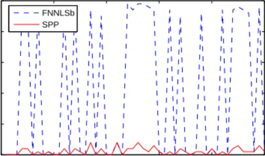
Before looking at the performance of AdSPP or AdBPP, we first compare the amount
of iterations required for each update for FNNLS and the single pivoting (SPP without
updating the inverse) discussed in section IV. Simulations were done with [0,1] uniformly distributed randomly generated data.
0 10 20 30 40 50 0 10 20 30 40 50 frame index (k) inner−iterations FNNLSb SPP
Figure 6.1: Number of inner-iterations required by FNNLSb vs. SPP per outer-iteration. Initial data size is 1000x100.
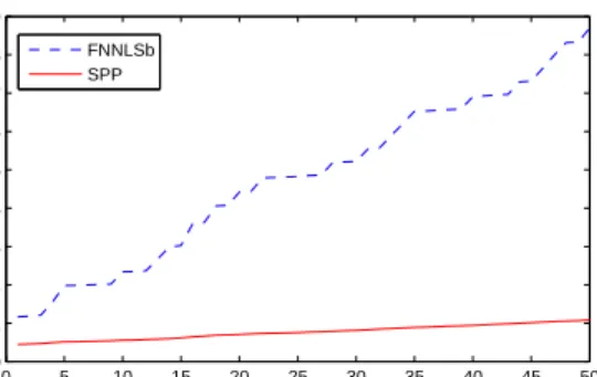
27 0 5 10 15 20 25 30 35 40 45 50 0 0.01 0.02 0.03 0.04 0.05 0.06 0.07 0.08 0.09 Data Stream cumulative run−time FNNLSb SPP
Figure 6.2: Cumulative run-time of FNNLSb vs. SPP corresponding to the simulation in Figure 6.1. Initial data size is 1000x100.
Even though both methods exchange one variable at a time, we see that the single pivoting method, as discussed in this paper, is more appropriate for warm starting a active-set based NNLS method. Although we abandon this method for the full exchange rule (which typically requires under two iterations in well initialized problems, such as here), these results provide some, otherwise unexpected, insight into the robustness of the pivoting style of [8] as opposed to the active-set approach.
Recognizing that FNNLSb performs poorly in this setting, we cease to include it in the following simulations. Figures 6.3 and 6.4 show the performance improvement of AdBPP over warm started BPP for updating the NNLS solution. We note that we also update the plain BPP algorithm with updates of the normal equation (this way, the comparisons are more fair with regards to efficiently tracking the passive set).
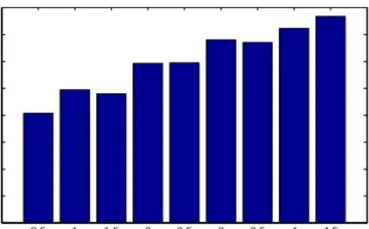
Comparing results in figures 6.3 and 6.4, we see that the speed improvement of AdBPP is much greater when the solution is more dense, and when the successive solutions experience minimal change in the support. By the end of the stream, the improvement of AdBPP in figure 6.3 is around 20%, whereas it is almost 50% in figure 6.3. This follows from the discussion in chapter 3. Figure 6.5 shows similar improvements for smaller,
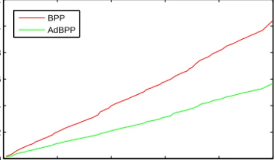
less over-determined data. We include an averaged speed improvement comparison
of AdBPP over BPP for in figure 6.6. In these experiments, we start with an MxN model size, and add 100 new data point. N is kept constant at 300 through all the experiments. The (initial) M is changed from 5,000 to 45,000, effectively changing how over-determined the system is. We see that AdBPP is best used for overdetermined
28 0 20 40 60 80 100 0 0.02 0.04 0.06 0.08 0.1 0.12 0.14 frame index (k) cumulative run−time AdSPP BPP AdBPP
Figure 6.3: AdBPP compared with warm started BPP. AdSPP also included for
refer-ence. Initial data size is 15,000x500. Final NP = 176. Average change in passive set
size per iteration is 1.37, with maximum change being 6.
0 20 40 60 80 100 0 0.02 0.04 0.06 0.08 0.1 0.12 frame index (k) cumulative run−time BPP AdBPP
Figure 6.4: AdBPP compared with warm started BPP. Initial data size is 50,000x300.
FinalNP = 219. Average change in passive set size per iteration is 0.24, with maximum
change being 2.
systems. At a certain level, the improvements start to saturate. This, however, seems to become more dependent on the system parameters such as cache size.
Admittedly, the performance gains appears less significant than the theoretical com-plexity order would lead one to believe. However, the updates used come with a higher memory read/write cost and must be implemented very efficiently for full benefits. Mem-ory/cache efficient code written in low level languages is expected to provide greater speed improvements.
29 0 10 20 30 40 50 60 70 80 90 100 0 0.002 0.004 0.006 0.008 0.01 0.012 0.014 0.016 frame index cumulative run−time BPP AdBPP
Figure 6.5: AdBPP compared with warm started BPP. Initial data size is 500x100.
Final NP = 43. Average change in passive set size per iteration is 1.57, with maximum
change being 5. 0.5 1 1.5 2 2.5 3 3.5 4 4.5 x 10⁴ 0 5 10 15 20 25 30 35 40 Initial M % improvement
Figure 6.6: Improvement of AdBPP over PBPP is compared for various data sizes.
6.2
NMF
We first present the results of the initialization described for the initialization of hk. In
the following table, three different initializations are compared. A random initialization (with a random support size), projected unconstrained LS (a commonly used one), and the proposed initialization. Starting with dimensions M = 50, N = 100, we add new frames, and test the total amount of iterations required for BPP to converge when
30
R: 10 20 30 40
Random: 133 193 215 238
Proposed: 75 135 174 191
LS: 0 20 48 76
Noting that the complexity of the LS initialization is O(M R2) versus O(N R), we see
the trade-off. The proposed initialization may only be worth it if N is not significantly larger than M, and if the expected support is small enough to justify the extra iterations of BPP.
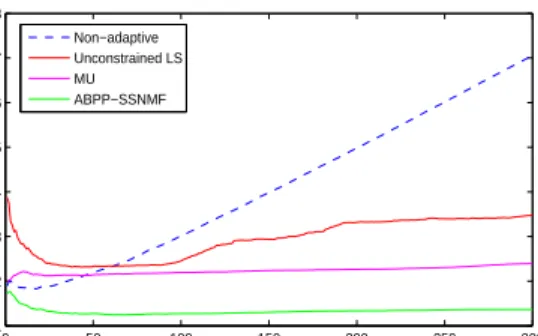
We now demonstrate the performance of AdBPP-SSNMF and compare it to the MU and ALS algorithms. Figure 6.7 demonstrates the running error of these algorithms on
a data stream. Initial data is generated from a random uniform [0,1] distribution. Each
new frame yi is generated from a uniform [0 + 0.1i,1 + 0.1i] distribution. This slight
shifting of the mean is done to simulate changing data (which would suggest necessity of
an adapting dictionary.) After the input of each frame, we calculate the activation hk,
update the dictionaryWk, and compute the running average of the following error
ek=kyk−Wkhkk2F (6.1)
This effectively describes the error in determining the activation of each new frame.
The initial factors W0 and H0 are initialized using (up to) 100 iterations of BPP. For
reference, a non-adaptive approach of supervised NMF described earlier is also included
in the comparison. For this, we always use W0 to determine hk without updating it.
We also note that for the MU implementation, the updative step for both Wk and
hk is done R times, so as to have comparable computational complexity with
AdBPP-SSNMF.
Not surprisingly, we see that when the incoming data slowly changes, using the old dic-tionary without updating it is not a good approach. Naturally, all of the semi-supervised methods tested here performed better than the non-supervised approach. The MU and AdBPP-SSNMF methods seem more stable than the ALS approach (this shouldn’t be surprising when recognizing the lack of optimality of ALS), with the AdBPP-SSNMF
31 0 50 100 150 200 250 300 1 2 3 4 5 6 7 8 frame index (k) error Non−adaptive Unconstrained LS MU ABPP−SSNMF
Figure 6.7: Comparison of online semi-supervised NMF using AdBPP-SSNMF, MU, ALS. Initial data size is M = 80, R = 50, N = 100.
method notably outperforming the former. We also note the number of rank-1 updates that had to be done using AdBPP-SSNMF and the number of LS problems that would have to be solved if plain block pivoting (without updating the inverses) was used.
AdBPP-SSNMF rank-1 updates: 12147
NMF-SS(BPP) LS problems : 9104
Although the ALS and MU algorithms are generally faster than AdBPP-SSNMF, the
latter shows significant performance improvements. Furthermore, utilization of the
discussed updates allows us to achieve a complexity of O(M R2) (worst case) when
updatingW, which is the bulk of the computation. Use of the standard BPP algorithm
would result in a complexity ofO(M N R2), making it more difficult to justify the
trade-off.
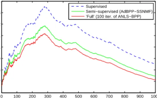
In the above comparison, we have looked at the error in determining each activation vector. We may, however, instead be interested in the full NMF error (5.2) at each step. In order to observe how the semi-supervised (using AdBPP-SSNMF) approach works
for this objective, we compare it to the supervised approach (updating only hk), and a
full NMF factorization method (100 iterations of ANLS-BPP), which updates all of W
and H(initialized on the previous data). Figure 6.8 shows such a comparison. For this,
the MovieLens database [25] is used. The matrix representation of this data presents users as rows, and movies as columns. Each entry in the matrix corresponds to a rating (1-5) by a given user for a movie (no rating signified by 0). The total data contains
32 943 users, and 1682 movies. Given NMF factors for a subset of the data, the goal is to update the factorization as each new movie (and corresponding user ratings) is added to the database. The factors are initialized with 100 iterations of BPP for 50 movies (using all the available users). 1000 new users are added, one by one, and the error in (5.2) compared between using the supervised, semi-supervised, and full NMF. We see that the semi-supervised approach (using the proposed method) actually achieves an NMF error only slightly higher than that of performing 100 iterations of BPP to update
all of W and H. This method may then serve as a good approximation to the NMF
problem in situations where updating the whole matrix His expensive.
0 100 200 300 400 500 600 700 800 900 1000 0.7 0.8 0.9 1 1.1 1.2 1.3 1.4 frame index error Supervised Semi−supervised (AdBPP−SSNMF) ’Full’ (100 iter. of ANLS−BPP)
Figure 6.8: Comparison of supervised, semi-supervised, and full NMF methods for updating NMF factors.
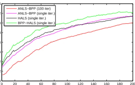
Lastly, we present the results to the complete NMF factorization. We compare the speed performance of HALS, BPP, and HALS-BPP hybrid (HALS on H, BPP on W), when warm-started with the previous solution and iterated only once. Neither of these three
methods were particularly sensitive to the initialization ofhk, so they were all initialized
in the same way. We first show the results of the full NMF error (5.2) (normalized to data size) at each iteration. All three methods are compared against doing ANLS-BPP until convergence (or for 100 iterations). We see that after only a single iteration at each time frame with either of these methods, the objective error stays within a close proximity of of the error of the ’complete’ (100 iterations) ANLS-BPP algorithm. Only
performing a single iteration, however, is much less computationally expensive. Of
33 0 20 40 60 80 100 120 140 160 180 200 0.018 0.02 0.022 0.024 0.026 0.028 0.03 0.032 0.034 frame index error ANLS−BPP (100 iter) ANLS−BPP (single iter.) HALS (single iter.) BPP−HALS (single iter.)
Figure 6.9: Comparison of singly iterated warm started ANLS-BPP, HALS, and HALS-BPP. Initial data size is M = 100, R = 30, N = 200.
For the same data size, we now compare the total run-times (in seconds) of the three discussed options for matrices of various densities. (The full ANLS-BPP run-time is not included, as it’s over 100s in all cases).
W and H dense W sparse, H dense W and H sparse
BPP 3.3610 3.7648 3.6375
HALS 0.6492 0.6523 0.6571
HALS-BPP 1.0437 0.9688 1.1054
Although one may expect ANLS-BPP to perform better in the sparse case and HALS-BPP to perform better in the half-sparse case, it seems HALS is always faster here. Changing data sizes and sparsity around tends to yield similar results. While, in the offline/batch setting, one may certainly find instances where ANLS-BPP outperforms HALS, but when updating to close solution, it seems that HALS reaps the computational benefits a bit more. In retrospect, this may not be too surprising. The ANLS-BPP method is typically more computationally intensive (from having to solve least squares problems), but can overcome this by converging more per iteration, due to the optimality of the updates for each block. When already given a good solution, however, this benefit is diminished.
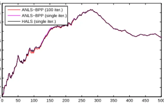
Finally, we run the same comparison on MovieLens data. As before, we begin with an initialization using 50 movies, and add new movies (500 this time), updating the solution with each new movie addition. We see that for this dataset, the solutions of all the algorithms actually converge to the same objective error very quickly. It seems
34 to serve as more motivation, then, that using only a single HALS iteration is a good approach for online NMF.
0 50 100 150 200 250 300 350 400 450 500 0.65 0.7 0.75 0.8 0.85 0.9 0.95 1 1.05 1.1 1.15 frame index error ANLS−BPP (100 iter.) ANLS−BPP (single iter.) HALS (single iter.)
Figure 6.10: Comparison of singly iterated warm started ANLS-BPP, HALS, and full ANLS-BPP for MovieLens data.
Chapter 7
Conclusion
This paper considered adaptive NNLS and NMF problems, which are of broad interest and find diverse applications in signal processing and well beyond. After reviewing the most commonly used methods for these problems, new techniques that improved on the computational efficiency and/or solution quality were developed.
First, a new single pivoting method for NNLS was discussed. While this method
wasn’t used for the best results, it shed some light on existing techniques. Further-more, the most efficient technique for NNLS was modified into an adaptive version (termed AdBPP) resembling the commonly studied RLS algorithm for unconstrained LS. This method showed to be advantageous under reasonable problem settings, and allowed for updating the NNLS solution recursively in the same complexity as RLS for unconstrained LS.
The method for NNLS was then applied to various adaptive NMF settings. It was shown to be applicable in settings where a complete factorization wasn’t required (or rather, wasn’t practical), and outperformed the MU and ALS algorithms that have been used in the similar settings. While we found its functional use in a complete adaptive NMF factorization restrictive, we explored other methods for this problem. We compared other possible ways to efficiently update the NMF factorization online, finally demonstrating what appears to be the most efficient method for this.
References
[1] DS Briggs. High fidelity interferometric imaging: Robust weighting and NNLS
deconvolution. InBulletin of the American Astronomical Society, volume 27, page
1444, 1995.
[2] Martin Slawski, Rene Hussong, Andreas Tholey, Thomas Jakoby, Barbara Grego-rius, Andreas Hildebrandt, and Matthias Hein. Isotope pattern deconvolution for peptide mass spectrometry by non-negative least squares/least absolute deviation
template matching. BMC Bioinformatics, 13(1):291, 2012.
[3] Mark H Van Benthem and Michael R Keenan. Fast algorithm for the solution of
large-scale non-negativity-constrained least squares problems. Journal of
chemo-metrics, 18(10):441–450, 2004.
[4] Anh Huy Phan Shunichi Amari Andrzej Cichocki, Rafal Zdunek. Nonnegative
Matrix and Tensor Factorizations: Applications to Exploratory Multi-way Data Analysis and Blind Source Separation. Wiley, 2009.
[5] Jingu Kim and Haesun Park. Toward faster nonnegative matrix factorization: A
new algorithm and comparisons. In Data Mining, 2008. ICDM’08. Eighth IEEE
International Conference on, pages 353–362. IEEE, 2008.
[6] Sijmen De Jong Rasmus Bro. A fast non-negativity-constrained least squares
algo-rithm. Journal of Chemometrics, 59:393–401, 1997.
[7] Richard. J. Hanson Charles. L. Lawson. Solving Least Squares Problems.
Prentice-Hall, 1974.
37 [8] Luis Vicente Luis Portugal, Joaquim Judice. A comparison between block-pivoting and interior point algorithms for linear least squares problems with non-negative
constraints. Mathematics of Computation, 63:625–643, 1994.
[9] Winifred J. Sherman, Jack; Morrison. Adjustment of an inverse matrix
correspond-ing to changes in a given column or a given row of the original matrix. The Annals
of Mathematical Statistics, (4):621, 12.
[10] Joan R Westlake. A handbook of numerical matrix inversion and solution of linear
equations. 1975.
[11] Yuancheng Luo and Ramani Duraiswami. Efficient parallel nonnegative least
squares on multicore architectures. SIAM Journal on Scientific Computing,
33(5):2848–2863, 2011.
[12] A. Bjorck. Stability analysis of the method of seminormal equations for linear least
squares problems. Linear Algebra and its Applications, 8889:31 – 48, 1987.
[13] Miroslav Rozlonk, Alicja Smoktunowicz, and Jiri Kopal. A note on iterative
re-finement for seminormal equations. Applied Numerical Mathematics, 75:167–174,
2014.
[14] Gene H Golub and Charles F Van Loan. Matrix computations, volume 3. JHU
Press, 2012.
[15] William W Hager. Updating the inverse of a matrix. SIAM Review, 31(2):221–239,
1989.
[16] Kyle A Gallivan, Michael Heath, Esmond Ng, B Peyton, Robert Plemmons,
C Romine, A Sameh, and R Voigt. Parallel algorithms for matrix computations,
volume 22. SIAM, 1990.
[17] Timothy A Davis and William W Hager. Row modifications of a sparse Cholesky
factorization. SIAM Journal on Matrix Analysis and Applications, 26(3):621–639,
38 [18] Pentti Paatero and Unto Tapper. Positive matrix factorization: A non-negative
factor model with optimal utilization of error estimates of data values.
Environ-metrics, 5(2):111–126, 1994.
[19] Seung H. Sebastian Lee, Daniel D. Learning the parts of objects by non-negative
matrix factorization. Nature, 401:788–791, 1999.
[20] Chih-Jen Lin. On the convergence of multiplicative update algorithms for
nonneg-ative matrix factorization. Neural Networks, IEEE Transactions on, 18(6):1589–
1596, 2007.
[21] Kejun Huang and N Sidiropoulos. Putting Nonnegative Matrix Factorization to the Test: A tutorial derivation of pertinent Cramer Rao bounds and performance
benchmarking. Signal Processing Magazine, IEEE, 31(3):76–86, 2014.
[22] Cyril Joder, Felix Weninger, Florian Eyben, David Virette, and Bj¨orn Schuller.
Real-time speech separation by semi-supervised nonnegative matrix factorization. InLatent Variable Analysis and Signal Separation, pages 322–329. Springer, 2012.
[23] C´edric F´evotte, Nancy Bertin, and Jean-Louis Durrieu. Nonnegative matrix
fac-torization with the Itakura-Saito divergence: With application to music analysis.
Neural computation, 21(3):793–830, 2009.
[24] LEE Seokjin, Sang Ha Park, and SUNG Koeng-Mo. On-line nonnegative matrix factorization method using recursive least squares for acoustic signal processing
sys-tems. IEICE TRANSACTIONS on Fundamentals of Electronics, Communications
and Computer Sciences, 94(10):2022–2026, 2011.