An Iterative Feature Perturbation Method for Gene Selection from Microarray Data

University of South Florida University of South Florida

Scholar Commons

Scholar Commons

Graduate Theses and Dissertations Graduate School

6-11-2010

An Iterative Feature Perturbation Method for Gene Selection from

An Iterative Feature Perturbation Method for Gene Selection from

Microarray Data

Microarray Data

Follow this and additional works at: https://scholarcommons.usf.edu/etd

Part of the American Studies Commons

Scholar Commons Citation Scholar Commons Citation

Canul Reich, Juana, "An Iterative Feature Perturbation Method for Gene Selection from Microarray Data" (2010). Graduate Theses and Dissertations.

An Iterative Feature Perturbation Method for Gene Selection from Microarray Data

by

Juana Canul Reich

A dissertation submitted in partial fulfillment of the requirements for the degree of

Doctor of Philosophy

Department of Computer Science & Engineering College of Engineering

University of South Florida

Major Professor: Lawrence O. Hall, Ph.D. Dmitry Goldgof, Ph.D.

Rafael Perez, Ph.D. Steven Eschrich, Ph.D.

Date of Approval: June 11, 2010

To my mother who will always be an inspiration throughout my life. To my husband for being my partner in life, who on top of his own job he strove his best at home while I was

at school. And, to my daughters Maru, Mine, and Vivi, who will always be my blessings from God. You all three represent my greatest commitments in life. I pray for wisdom so I can accomplish my job as your mother. All together, we have survived throughout this,

Acknowledgements

My first acknowledgement is to God for being my source of spiritual strength.

I would like to acknowledge those agencies who in different ways supported my PhD studies: Fulbright, Promep, Conacyt, UJAT, UJAT-DAIS, Moffitt Cancer Center and Re-search Institute, and USF. My endless gratitude to Dr. Hall, Dr. Goldgof, and Dr. Eschrich for their valuable week-after-week advice. To my family, for walking along with me all this time.

Last but not less, my heart is with those people we met in Tampa, now friends of my family, who made of our stay an unforgettable and pleasant one.

Table of Contents

List of Tables v

List of Figures viii

Abstract xiii Chapter 1 Introduction 1 1.1 Motivation 1 1.2 Contributions 3 1.3 Organization 4 Chapter 2 Background 5 2.1 Microarray Data 5 2.2 Feature Selection 6 2.2.1 Filters 7 2.2.1.1 Student’s T-Test 7 2.2.1.2 Information Gain 8 2.2.1.3 ReliefF 9 2.2.2 Wrappers 10 2.2.3 Embedded Methods 11

2.3 Support Vector Machines 12 Chapter 3 Feature Selection Methods for Microarray Data 16

3.1 Filters 16

3.1.1 Student’s T-Test 16

3.1.2 Rank Products 17

3.1.3 Markov Blanket and ROC Curves 19 3.1.4 Information Gain, ReliefF, and Correlation-Based

Fea-ture Selection 21

3.2 Wrappers 23

3.2.1 Sequential Search 23

3.2.2 Genetic Algorithms and Local Search 24

3.3 Embedded 26

3.3.1 Recursive Feature Elimination (SVM-RFE) 26

3.3.2 Random Forests 28

3.3.3 Penalized Methods: HHSVM 30

3.3.4 Local Learning Based Feature Selection 31 Chapter 4 Iterative Feature Perturbation Method 34

4.1 Binary Search 36

4.2 Computational Cost of IFP 38

Chapter 5 Experimental Studies 40

5.1 Data and Preprocessing 40

5.3 Performance Measure 42 5.4 Adaptive Feature Elimination Strategy 43

5.5 Gene Pre-Filtering Strategy 44

5.6 Experiments and Results 44

5.6.1 Accuracy Results 45

5.6.2 Intersection Across the Entire Set of Features 47

5.6.3 Gene Preselection 54

5.6.4 Intersection Across a Subset of Features (Genes) 60 5.7 Frequency of the Use of SVM Weights for Tie-Breaking by

IFP 66

5.8 AUC Analysis 66

5.8.1 Across the Entire Set of Features 67 5.8.2 Across the Top 200 Subset of Features 69

Chapter 6 Statistical Analysis 71

6.1 Starting with the Entire Set of Features 72 6.2 Starting with a Preselected Set of n Features 75 6.3 Preselection vs. No Preselection of IFP and SVM-RFE 79 Chapter 7 Filtering for Improved Gene Selection 83 7.1 Experimental Design and Evaluation 83 7.2 Effect of Filtering in Terms of SVM Accuracy 84 7.3 Accuracy of IFP and SVM-RFE Using Filtered Datasets 87 7.4 Statistical Comparison of Filtering Methods 95

7.5 Analysis of Overlap Between Genes Selected 99 7.6 Summary of Results Including Reviewed Feature Selection

Methods 104

Chapter 8 Ensemble Approach Using Bagging 110

8.1 Defining Ensemble and Bagging 110

8.2 Why Use Bagging? 111

8.3 Bagging Applied to IFP, SVM-RFE, and the T-Test 112

8.3.1 Colon Cancer Dataset 113

8.3.2 Leukemia Dataset 114

8.3.3 Moffitt Colon Cancer Dataset 114

Chapter 9 Discussion and Future Work 120

9.1 Future Work 123

List of References 124

Appendices 133

Appendix A: Flowchart for Iterative Feature Perturbation Method 134 Appendix B: Accuracies for the Top N Features with P Values <= 0.01 135

List of Tables

Table 5.1 Confusion matrix. 43

Table 5.2 AUC analysis of accuracy curves across all 4 datasets using the entire

set of features. 68

Table 5.3 AUC analysis of accuracy curves across all 4 datasets using the top

200 features. 70

Table 6.1 Statistical analysis of results on the colon cancer dataset between the methods IFP (I), SVM-RFE (R), and the t-test (T) across features (a) 50 to 38, (b) 37 to 25, (c) 24 to 12, and (d) 11 to 1 with no previous

preselection of features. 73

Table 6.2 Statistical analysis of results on the leukemia dataset between the methods IFP (I), SVM-RFE (R), and the t-test (T) across features (a)

24 to 12 and (b) 11 to 1 with no previous preselection of features. 74 Table 6.3 Statistical analysis of results on the colon cancer dataset between the

methods IFP (I), SVM-RFE (R), and the t-test (T) across features (a) 50 to 38, (b) 37 to 25, (c) 24 to 12, and (d) 11 to 1 with previous

preselection of n features (those with p values<=0.01). 76 Table 6.4 Statistical analysis of results on the leukemia dataset between the

methods IFP (I), SVM-RFE (R), and the t-test (T) across features (a) 50 to 38, (b) 37 to 25, (c) 24 to 12, and (d) 11 to 1 with previous

preselection of n features (those with p values<=0.01). 78 Table 6.5 Statistical analysis of results on the lung cancer dataset between the

methods IFP (I), SVM-RFE (R), and the t-test (T) across features (a) 33 to 21, (b) 20 to 8, and (c) 7 to 1 with previous preselection of n

Table 6.6 Statistical comparison between doing preselection (P) and not doing preselection (NP) with the methods IFP and SVM-RFE across fea-tures (a) 50 to 38, (b) 37 to 25, (c) 24 to 12, and (d) 11 to 1 on the

colon cancer dataset. 80

Table 6.7 Statistical comparison between doing preselection (P) and not do-ing preselection (NP) with the methods IFP and SVM-RFE across features (a) 32 to 20, (b) 19 to 7, and (c) 6 to 1 on the lung cancer

dataset. 82

Table 7.1 Highest accuracies attained for each dataset across three filters. 90 Table 7.2 AUC analysis of accuracy curves across all four filtered datasets,

using the (a) t-test, (b) information gain, and (c) ReliefF. 98 Table 7.3 Average accuracy improvements obtained between IFP and

SVM-RFE applied to the four original non-filtered datasets and to IFP and

SVM-RFE applied to the 200-gene filtered datasets. 101 Table 7.4 Statistical comparison across the top 50 features of the accuracies

from IFP on the best 200 genes filtered according to the t-test (T),

information gain (G), and ReliefF (F) for the four datasets. 101 Table 7.5 Statistical comparison across the top 50 features of the accuracies

from SVM-RFE on the best 200 genes filtered according to the t-test

(T), information gain (G), and ReliefF (F) for the four datasets. 102 Table 7.6 Statistical comparison across the top 50 features of the accuracies

from SVM on the best 200 genes filtered according to the t-test (T),

information gain (G), and ReliefF (F) for the four datasets. 102 Table 7.7 Percentage of intersection (at 50 genes) between genes selected by

IFP and SVM-RFE when applied on the top 200 genes filtered with

the t-test, information gain, and ReliefF across the four datasets. 103 Table 7.8 Percentage of intersection (at 50 genes) of genes filtered by (a) IFP

and (b) SVM-RFE with the genes filtered by each filter across the

four datasets. 103

Table 7.9 Percentage of intersection (at 50 genes) between genes filtered by any

Table 7.10 Percentage of intersection (at 50 genes) for each method with it-self using the (a) information gain, (b) ReliefF, and (c) t-test, across the top 200 genes filtered with the corresponding filter for the four

datasets. 104

Table 7.11 Summary of results from feature selection methods in [5, 9–11] for

the colon cancer dataset. 106

Table 7.12 Summary of results from feature selection methods in [12, 47] and

this work for the colon cancer dataset. 107 Table 7.13 Summary of results from feature selection methods in [5, 8–10] for

the leukemia dataset. 108

Table 7.14 Summary of results from feature selection methods in [11, 12, 44]

List of Figures

Figure 2.1 Matrix representation of a microarray dataset [3]. 6 Figure 2.2 Filters work independently of the learning algorithm [15]. 7

Figure 2.3 Algorithm ReliefF [23]. 10

Figure 2.4 Wrappers use the learning algorithm as a black box when evaluating

feature subsets [15]. 11

Figure 2.5 Embedded methods incorporate the feature subset search and

evalua-tion when building a classifier. 11

Figure 2.6 Illustration of a feature mapping via a kernel function(Φ). 12 Figure 2.7 Maximum margin hyperplane (H0). 13

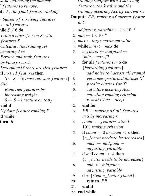
Figure 4.1 IFP algorithm. 39

Figure 5.1 Comparison of resulting average weighted accuracy of feature rank-ing given by methods IFP, SVM-RFE, and the t-test for the colon

cancer dataset. 47

Figure 5.2 Comparison of resulting average weighted accuracy of feature rank-ing given by methods IFP, SVM-RFE, and the t-test for the leukemia

dataset. 48

Figure 5.3 Comparison of resulting average weighted accuracy of feature rank-ing given by methods IFP, SVM-RFE, and the t-test for the Moffitt

Figure 5.4 Comparison of resulting average weighted accuracy of feature rank-ing given by methods IFP, SVM-RFE, and the t-test for the lung

cancer dataset. 50

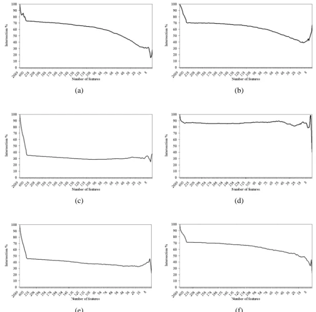
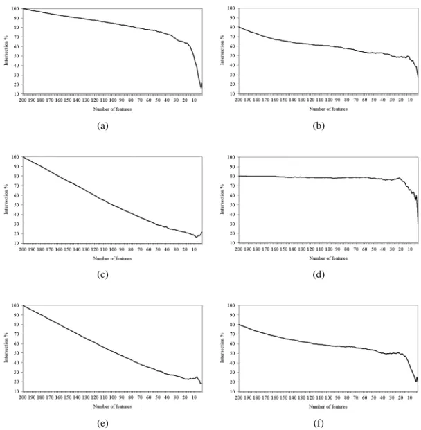
Figure 5.5 Intersection across the entire set of features of (a) IFP vs. SVM-RFE, (b) IFP vs. IFP, (c) t-test vs. IFP, (d) t-test vs. t-test, (e) t-test vs. SVM-RFE, and (f) SVM-RFE vs. SVM-RFE on the colon cancer

dataset. 51

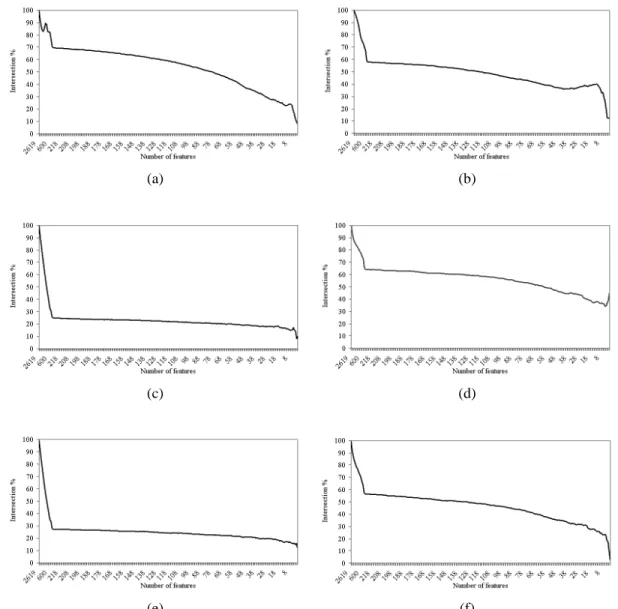
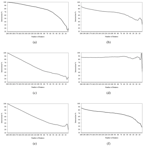
Figure 5.6 Intersection across the entire set of features of (a) IFP vs. SVM-RFE, (b) IFP vs. IFP, (c) t-test vs. IFP, (d) t-test vs. t-test, (e) t-test vs. SVM-RFE, and (f) SVM-RFE vs. SVM-RFE on the leukemia

dataset. 53

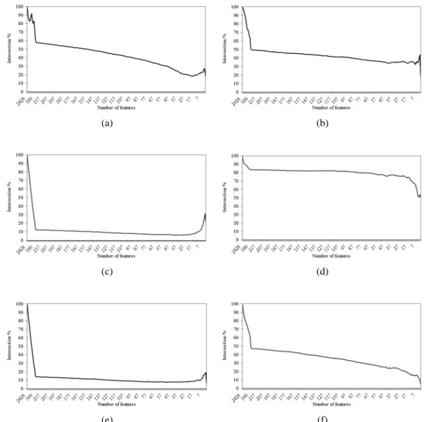
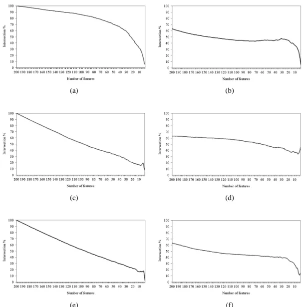
Figure 5.7 Intersection across the entire set of features of (a) IFP vs. SVM-RFE, (b) IFP vs. IFP, (c) t-test vs. IFP, (d) t-test vs. t-test, (e) t-test vs. SVM-RFE, and (f) SVM-RFE vs. SVM-RFE on the Moffitt colon

cancer dataset. 54

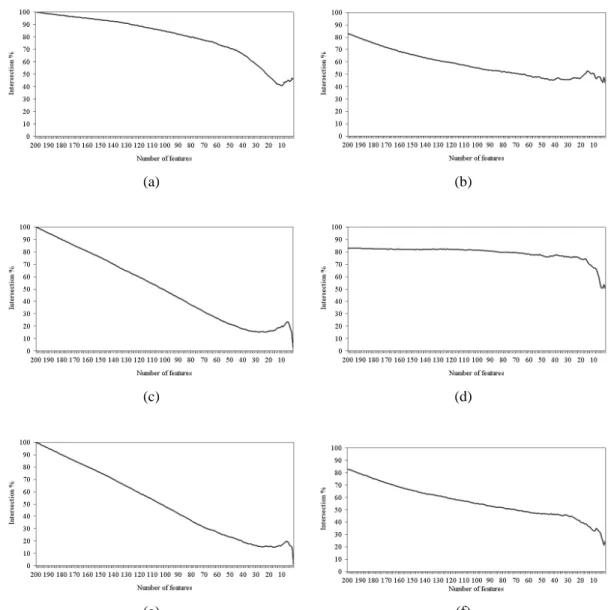
Figure 5.8 Intersection across the entire set of features of (a) IFP vs. SVM-RFE, (b) IFP vs. IFP, (c) t-test vs. IFP, (d) t-test vs. t-test, (e) t-test vs. SVM-RFE, and (f) SVM-RFE vs. SVM-RFE on the lung cancer

dataset. 55

Figure 5.9 Comparison of resulting average weighted accuracy of feature rank-ing given by methods IFP, SVM-RFE, and the t-test for the colon

cancer dataset across top 200 features as filtered by t-test. 56 Figure 5.10 Comparison of resulting average weighted accuracy of feature

rank-ing given by methods IFP, SVM-RFE, and the t-test for the leukemia

dataset across top 200 features as filtered by t-test. 57 Figure 5.11 Comparison of resulting average weighted accuracy of feature

rank-ing given by methods IFP, SVM-RFE, and the t-test for the Moffitt

colon cancer dataset across top 200 features as filtered by t-test. 58 Figure 5.12 Comparison of resulting average weighted accuracy of feature

rank-ing given by methods IFP, SVM-RFE, and the t-test for the lung

Figure 5.13 Intersection across the top 200 subset of features of (a) IFP vs. SVM-RFE, (b) IFP vs. IFP, (c) t-test vs. IFP, (d) t-test vs. t-test, (e) t-test vs. SVM-RFE, and (f) SVM-RFE vs. SVM-RFE on the colon cancer

dataset. 61

Figure 5.14 Intersection across the top 200 subset of features of (a) IFP vs. SVM-RFE, (b) IFP vs. IFP, (c) t-test vs. IFP, (d) t-test vs. t-test, (e) t-test vs. SVM-RFE, and (f) SVM-RFE vs. SVM-RFE on the leukemia

dataset. 62

Figure 5.15 Intersection across the top 200 subset of features of (a) IFP vs. SVM-RFE, (b) IFP vs. IFP, (c) t-test vs. IFP, (d) t-test vs. t-test, (e) t-test vs. SVM-RFE, and (f) SVM-RFE vs. SVM-RFE on the Moffitt colon

cancer dataset. 63

Figure 5.16 Intersection across the top 200 subset of features of (a) IFP vs. SVM-RFE, (b) IFP vs. IFP, (c) t-test vs. IFP, (d) t-test vs. t-test, (e) t-test vs. SVM-RFE, and (f) SVM-RFE vs. SVM-RFE on the lung cancer

dataset. 65

Figure 7.1 SVM accuracy across the top 200 genes filtered with the t-test,

infor-mation gain, and ReliefF for the colon cancer dataset. 85 Figure 7.2 SVM accuracy across the top 200 genes filtered with the t-test,

infor-mation gain, and ReliefF for the leukemia dataset. 86 Figure 7.3 SVM accuracy across the top 200 genes filtered with the t-test,

infor-mation gain, and ReliefF for the Moffitt colon cancer dataset. 87 Figure 7.4 SVM accuracy across the top 200 genes filtered with the t-test,

infor-mation gain, and ReliefF for the lung cancer dataset. 88 Figure 7.5 Comparison of resulting average weighted accuracy of feature

rank-ing given by methods IFP, SVM-RFE and information gain (in terms of SVM classifier accuracy) on the colon cancer dataset across top

200 features as filtered by information gain. 90 Figure 7.6 Comparison of resulting average weighted accuracy of feature

rank-ing given by methods IFP, SVM-RFE and ReliefF (in terms of SVM classifier accuracy) on the colon cancer dataset across top 200

Figure 7.7 Comparison of resulting average weighted accuracy of feature rank-ing given by methods IFP, SVM-RFE and information gain (in terms of SVM classifier accuracy) on the leukemia dataset across top 200

features as filtered by information gain. 92 Figure 7.8 Comparison of resulting average weighted accuracy of feature

rank-ing given by methods IFP, SVM-RFE and ReliefF (in terms of SVM classifier accuracy) on the leukemia dataset across top 200 features as

filtered by ReliefF. 93

Figure 7.9 Comparison of resulting average weighted accuracy of feature rank-ing given by methods IFP, SVM-RFE and information gain (in terms of SVM classifier accuracy) on the Moffitt colon cancer dataset across

top 200 features as filtered by information gain. 94 Figure 7.10 Comparison of resulting average weighted accuracy of feature

rank-ing given by methods IFP, SVM-RFE and ReliefF (in terms of SVM classifier accuracy) on the Moffitt colon cancer dataset across top 200

features as filtered by ReliefF. 95

Figure 7.11 Comparison of resulting average weighted accuracy of feature rank-ing given by methods IFP, SVM-RFE and information gain (in terms of SVM classifier accuracy) on the lung cancer dataset across top 200

features as filtered by information gain. 96 Figure 7.12 Comparison of resulting average weighted accuracy of feature

rank-ing given by methods IFP, SVM-RFE and ReliefF (in terms of SVM classifier accuracy) on the lung cancer dataset across top 200 features

as filtered by ReliefF. 97

Figure 7.13 Comparison of AUC values corresponding to the average accuracy curves of IFP applied across the top 200 genes filtered with the t-test,

information gain, and ReliefF for each dataset. 99 Figure 7.14 Comparison of AUC values obtained with SVM-RFE across the top

200 genes filtered with the t-test, information gain, and ReliefF for

each dataset. 100

Figure 8.1 IFP bagged accuracy in comparison with IFP and SVM-RFE (highest

Figure 8.2 SVM-RFE bagged accuracy in comparison with SVM-RFE (highest

accuracy achieved) for the colon cancer dataset. 114 Figure 8.3 t-test bagged accuracy in comparison with the t-test (in terms of SVM

classifier accuracy) and SVM-RFE (highest accuracy achieved) for

the colon cancer dataset. 115

Figure 8.4 IFP bagged accuracy in comparison with IFP and the t-test (in terms of SVM classifier accuracy), which achieved the highest accuracy for

the leukemia dataset. 116

Figure 8.5 SVM-RFE bagged accuracy in comparison with SVM-RFE and the t-test (in terms of SVM classifier accuracy), which achieved the highest

accuracy for the leukemia dataset. 117

Figure 8.6 t-test bagged accuracy in comparison with the t-test (in terms of SVM

classifier accuracy) for the leukemia dataset. 118 Figure 8.7 IFP bagged accuracy in comparison with IFP and the t-test (in terms

of SVM classifier accuracy), which achieved the highest accuracy for

the Moffitt colon cancer dataset. 118

Figure 8.8 SVM-RFE bagged accuracy in comparison with SVM-RFE and the t-test (in terms of SVM classifier accuracy), which achieved the highest

accuracy for the Moffitt colon cancer dataset. 119 Figure 8.9 t-test bagged accuracy in comparison with the t-test (in terms of SVM

classifier accuracy) for the Moffitt colon cancer dataset. 119

Figure A.1 Flowchart of IFP. 134

Figure B.1 Comparison of resulting average weighted accuracy of IFP, SVM-RFE, and the t-test across the top n features with p values <= 0.01 for

An Iterative Feature Perturbation Method for Gene Selection from Microarray Data

Juana Canul Reich ABSTRACT

Gene expression microarray datasets often consist of a limited number of samples relative to a large number of expression measurements, usually on the order of thousands of genes. These characteristics pose a challenge to any classification model as they might negatively impact its prediction accuracy. Therefore, dimensionality reduction is a core process prior to any classification task.

This dissertation introduces the iterative feature perturbation method (IFP), an embed-ded gene selector that iteratively discards non-relevant features. IFP considers relevant features as those which after perturbation with noise cause a change in the predictive accuracy of the classification model. Non-relevant features do not cause any change in the predictive accuracy in such a situation.

We apply IFP to 4 cancer microarray datasets: colon cancer (cancer vs. normal), leukemia (subtype classification), Moffitt colon cancer (prognosis predictor) and lung can-cer (prognosis predictor). We compare results obtained by IFP to those of SVM-RFE and the t-test using a linear support vector machine as the classifier in all cases. We do so using the original entire set of features in the datasets, and using a preselected set of 200

features (based on p values) from each dataset. When using the entire set of features, the IFP approach results in comparable accuracy (and higher at some points) with respect to SVM-RFE on 3 of the 4 datasets. The simple t-test feature ranking typically produces classifiers with the highest accuracy across the 4 datasets. When using 200 features chosen by the t-test, the accuracy results show up to 3% performance improvement for both IFP and SVM-RFE across the 4 datasets. We corroborate these results with an AUC analysis and a statistical analysis using the Friedman/Holm test.

Similar to the application of the t-test, we used the methods information gain and reliefF as filters and compared all three. Results of the AUC analysis show that IFP and SVM-RFE obtain the highest AUC value when applied on the t-test-filtered datasets. This result is additionally corroborated with statistical analysis.

The percentage of overlap between the gene sets selected by any two methods across the four datasets indicates that different sets of genes can and do result in similar accuracies.

We created ensembles of classifiers using the bagging technique with IFP, SVM-RFE and the t-test, and showed that their performance can be at least equivalent to those of the non-bagging cases, as well as better in some cases.

Chapter 1: Introduction

Gene expression microarray datasets tend to be small in sample size due to the cost associated with the assays. Typically, there are many more gene expression measurements (e.g. 54,000 transcripts) available than samples. Hence, the selection of a subset of genes/features is crucial before building a classifier. Identifying a small number of genes that are good predictors is important from a biological standpoint, as expression experi-ments are typically performed to generate hypotheses for further experimentation in the lab [1]. For clinical applications, identifying a small number of genes that are important in predicting patient survival time or diagnosing cancer can speed the translation of expression signatures into cost-effective tests for clinical practice. From a machine learning viewpoint, too many features/genes in a dataset can negatively influence the classification performance as they increase the possibility of overfitting. Therefore, the feature selection process plays a vital role for the building of a successful classifier from microarray datasets.

1.1 Motivation

Feature selection on microarray datasets is primarily conducted to select relevant genes amongst the usually numerous genes present in this type of data [2, 3]. This process aids in other aspects such as general data reduction; performance improvement since less genes

lead to a reduced risk of overfitting, as well as learning algorithms that are able to work faster with less amount of data; and for data understanding and visualization since for example it is simpler to visualize a reduced dataset [2].

On the other hand, most learning algorithms existing before the advent of microarray analysis have not been designed to cope with high dimensional and small sample size characteristics. Microarray analysis raises the need for a special feature selection process prior to analysis of data.

Currently, in bioinformatics the feature selection process has become a prerequisite for model building, since by nature tasks such as sequence analysis, microarray analysis, and spectral analysis deal with high dimensional data. As a result, diverse feature selection techniques have appeared in this field [4].

Three commonly used approaches for feature selection are filters, wrappers, and em-bedded methods [4]. Filters typically will evaluate each gene in isolation without consid-ering correlation between genes. A filter will rank all genes based on their capability of discriminating the target class and eventually the top n genes get selected [3]. Examples of univariate filters are the t-test [5] and rank products [6]. Multivariate filters consider inter-action between genes; examples are the Markov blanket filter [7] and the correlation-based feature selection [8]. Wrappers and embedded feature selection methods are multivariate since they search for subsets of genes. Examples of wrappers are applied in [9, 10], and examples of embedded methods are applied in [11–13]. A summary of results obtained with these approaches is shown and discussed in Section 7.6.

1.2 Contributions

This dissertation contributes to the state-of-the-art of the gene selection methods with the introduction of the Iterative Feature Perturbation (IFP) method. IFP is an embedded gene selector with the capability of using any classification algorithm as the base classifier. All experiments with IFP in comparison with the Recursive Feature Elimination (SVM-RFE), and the t-test feature ranking are conducted on four microarray cancer datasets using SVM as the base classifier in all cases. Experiments include, first the use of the entire set of genes of each dataset, and second the use of a subset of preselected genes ranked with basis on their p values (from the t-test). We show that accuracy improvements can be obtained as a result of gene preselection. For both scenarios, statistical analysis is conducted to determine the significance level of differences detected in the accuracy results. The Area Under the accuracy Curve (AUC) from each method is used as a measure for comparison between methods as well.

The intersection or amount of overlap between genes selected by two methods at points where similar accuracies are observed is analyzed, and the conclusion is made that different sets of genes can lead to the same or similar accuracies. It is also true, that a high percentage of overlap between genes selected does not guarantee similar performance. This suggests better feature selection methods that find unique sets or a better biological model are needed.

Experiments are conducted using filters such as the information gain and ReliefF in addition to the t-test. Performance comparisons of IFP and SVM-RFE applied to the 12 filtered datasets (4 datasets and 3 filters) are made in terms of the AUC measure. Statistical analysis is conducted in the accuracy results. Based on our results we conclude that the

t-test can be at least as accurate as other filter methods and we suggest that it should be considered for feature selection on microarray data. It provides a simple approach for comparison purposes.

Ensemble of classifiers typically improve performance. We show that accuracy im-provements can be attained by building ensembles of 30 bagged classifiers for each of IFP, SVM-RFE and the t-test using SVMs.

1.3 Organization

This dissertation is presented as follows. In Chapter 2 background concepts related to the topic of microarray data, feature selection as well as support vector machines are discussed. Chapter 3 presents some feature selection techniques commonly used in the microarray domain. Chapter 4 introduces the Iterative Feature Perturbation method. Chap-ter 5 provides a thorough description of experimental studies conducted using IFP, SVM-RFE, and the t-test for feature selection across four microarray cancer datasets. Results are presented in terms of accuracy, overlap of genes selected between each pair of methods, as well as in terms of the AUC measure, for two scenarios: 1) using the entire set of genes of each dataset and 2) using prefiltered datasets. Chapter 6 shows the statistical analysis conducted on results presented in Chapter 5. Chapter 7 presents results of experiments conducted using information gain, and ReliefF as filter methods in comparison with the t-test. Chapter 8 discusses the use of bagging for an ensemble approach including 30 classifiers for each method IFP, SVM-RFE, and the t-test. Chapter 9 summarizes the work presented and outlines future directions.

Chapter 2: Background

This chapter reviews some concepts related to the investigated problem. Microarray data, feature selection, classification of feature selection methods, and support vector ma-chines are briefly described. The three filters later used in experiments are described here.

2.1 Microarray Data

Microarray analyses are motivated by the search for useful patterns of tumor classifi-cation, disease state classificlassifi-cation, discovery of new subtypes of disease or disease states, among others. Microarray data are characterized as having a large number of features/genes typically on the order of thousands, in contrast to a small number of samples usually on the order of tens or hundreds, and redundancy among genes. A matrix representation of a dataset is shown in Figure 2.1. Each row represents a sample and each column a gene. Each entry shows a number which is the level of expression of a particular gene in a particular sample. The last column to the right shows the label or class that each sample belongs to. Microarray studies often involve the use of machine learning methods such as unsupervised and supervised learning. Unsupervised learning finds subgroups in the data based on a similarity measure between the expression profiles. It does not consider any prior knowledge or classification information to accomplish its goal, that is, it does not use

Figure 2.1: Matrix representation of a microarray dataset [3].

the class column of a dataset. As a result of unsupervised learning, unknown subtypes of tumors may be found. Supervised learning on the other hand, starts with sets of samples known to be associated with a particular disease or diseases (it does require a class column of a dataset), and searches for a pattern of expression or rules. These rules will help classify unseen samples [14].

2.2 Feature Selection

The high dimensionality and redundancy in microarray datasets make the classification task challenging [3]. The problem is some learning algorithms may perform poorly when dealing with data that has a number of irrelevant features [15]. So, in microarray applica-tions there is a need to select a subset of features (genes) to be used by the classification algorithm when creating a model, such that a model that does not overfit and achieves the highest accuracy possible is chosen. Also, learning algorithms work faster on datasets with fewer features.

The feature selection methods can be categorized into filters, wrappers, and embedded methods [4, 13].

2.2.1 Filters

Filters select features based on a measure/score individually obtained on each feature (univariate case) [15]. Low-scoring features are then discarded and only a subset of selected features is given as input to the learning algorithm. Filters do not incorporate the learning algorithm in the feature subset search, they only look at properties of the data. In other words, filters select subsets of features independently of the learning algorithm as illus-trated in Fig. 2.2. Advantages of filters are that they are computationally efficient to deal with very high dimensional datasets, and they are simple to compute. A disadvantage is that filters do not account for feature dependencies. Multivariate filters aim at incorporating feature dependencies [4, 16].

Figure 2.2: Filters work independently of the learning algorithm [15].

There are three filters used in a portion of the experiments conducted in this work which are described below. The filters are the Student’s t-test, information gain, and ReliefF.

2.2.1.1 Student’s T-Test

The t-test [5, 17, 18] is a statistical hypothesis test used to determine the significance of the difference between the means of two independent samples. It assumes normally distributed populations. For unequal variance and unequal (may be equal) sample sizes the

t statistic is calculated as follows

t= qX¯1−X¯2

s2₁ n1+

s2₂ n2

where ¯X1and ¯X2are the means of the two samples; s21and s22are the variance estimates of the two samples; n1and n2are the sample sizes of the two samples.

The degrees of freedom df can be calculated as

d f = [ s2₁ n1+ s2₂ n2] 2 (s2₁/n1)2 n1−1 + (s2₂/n2)2 n2−1

The t distribution can be used with the t statistic and df degrees of freedom as param-eters to calculate the corresponding p value. In this work we use an R library [19] that implements the t distribution. When the t-test is used as a filter, a p value for each feature in the dataset is generated. Features are then ranked according to p values. The smaller the p value the more relevant the feature.

2.2.1.2 Information Gain

The information gain from information theory was described by Quinlan in [20]. This filter evaluates the worth of a feature/gene by measuring the information gain with respect to the class. Features can be ranked in decreasing information gain order and those with the largest information gain are selected. Information gain is defined by [20–22]

In f oGain(X|Y) =H(X)−H(X|Y),

where H(X) is the entropy of X, which is defined as

H(X) =−∑iP(xi)log2(P(xi)),

where P(xi)is the prior probabilities for all values of X,

H(X|Y) =−∑_jP(yj)∑iP(xi|yj)log2(P(xi|yj)),

where P(xi|yj)is the posterior probability of xi given the value of yj.

In terms of classes and attributes, the information gain measure is expressed as

In f oGain(Class|Attribute) =H(Class)−H(Class|Attribute).

2.2.1.3 ReliefF

The ReliefF algorithm was described by Kononenko in [23, 24]. It is used to estimate the quality of attributes based on the criterion of how well their values distinguish among instances of different classes. ReliefF estimates probabilities more reliably and is able to deal with incomplete (missing values) and multi-class datasets.

Given an instance (and for each training instance), ReliefF searches for its k nearest neighbors: k nearest hits (instances from the same class) and k nearest misses (instances from each different class), and averages the contribution of all k nearest hits/misses. k is a user-defined value which, as proposed by the authors in [23] can be used with a default value k=10 with satisfactory results (k=10 was used for experiments with ReliefF in this work). The average contribution of all near misses is weighted with the prior probabilities of each class.

Function diff(Attribute,Instance1,Instance2) calculates the difference between the val-ues of Attribute for two instances. Feature weights are calculated as shown in Fig. 2.3, and they are estimates of the quality of features (attributes). The logic behind the weight formulation is that a good attribute should have the same value for instances from the same

set all weights W[A]:=0.0;

for i :=1 to n do

randomly select an instance R; find k nearest hits Hj

for each class C6=class(R)do

find k nearest misses Mj(C);

end for for A :=1 to #attributes do W[A]:=W[A]− k

∑

∑

∑

Figure 2.3: Algorithm ReliefF [23].

class and should differentiate between instances from different classes. The pseudocode for ReliefF is shown in Fig. 2.3.

2.2.2 Wrappers

For wrappers, the feature subset search incorporates a learning algorithm to assess diverse feature subsets as shown in Fig. 2.4. The subset with the best assessment is chosen [15]. There is a search algorithm which searches through the search space for the optimal feature subset according to some criteria. However as the number of features increases, the number of possible feature subsets grows exponentially. Heuristic search methods can be used in guiding the search. An advantage of wrappers is that they account for feature dependencies. A disadvantage is that wrappers are computationally intensive as they require training a model for each potential feature subset [2, 4].

Figure 2.4: Wrappers use the learning algorithm as a black box when evaluating feature subsets [15].

2.2.3 Embedded Methods

Embedded methods incorporate the feature subset search and evaluation in the process of building a classifier [2] as shown in Fig. 2.5. The search is guided by the learning algorithm. Embedded methods are computationally less intensive than wrappers and they account for feature dependencies.

Figure 2.5: Embedded methods incorporate the feature subset search and evaluation when building a classifier.

2.3 Support Vector Machines

Data with characteristics of high dimensionality and small number of samples can be handled with SVMs [25], and particularly linear SVM kernels have been used for microarray data [11], [26], [27]. SVMs were introduced by Vapnik [28]. A thorough description of SVMs can be found in [29, 30].

SVMs map 2-class training data termed the input space into a higher dimensional space termed the feature space by applying a kernel function (see Fig. 2.6), and find a maximum margin hyperplane in the feature space that separates the data into the two classes. The maximum margin hyperplane has the largest distance from the hyperplane to the closest training points [26]. By maximizing the margin between the two classes the classification performance improves [31].

Figure 2.6: Illustration of a feature mapping via a kernel function(Φ). The hyperplane in the feature space corresponds to a non-linear decision boundary in the input space [21, 32].

Fig. 2.7 shows an example of a maximum margin hyperplane. Support vectors are the training samples which define the margin boundaries. SVM training has the form of a quadratic programming dual problem [34]:

Figure 2.7: Maximum margin hyperplane (H0). H1and H2are the margin boundaries. Support vectors are the training samples that fall on H1and H2[33].

maximize: l

∑

∑

∑

where l is the number of training samples, yi is the class/label (+1 for positive and -1 for

function for the ith and jth samples. C is the regularization parameter chosen by the user and represents the penalty to errors. When C is set to small values, errors are allowed and a much larger margin is obtained by the SVM [27]. The prediction of the SVM for a sample

x is f(x) =sign( l

∑

where the scalar value b and the vector of alphasα (with l elements) are determined by the quadratic optimization problem.

The weight of each feature [29] is calculated as follows

w=

nSV

∑

i=1

αiyixi (2.5)

where nSV is the number of support vectors which are the only training samples with nonzero alpha values, yiis the label/class (+1/-1) for the ith support vector,αiis a positive

real value given by the SVM model to the ith support vector indicating its contribution to

the margin, and xiis the gene/feature value in the ith support vector.

The nonlinear mapping of the input space into the feature space simply requires the evaluation of dot products between the samples in the input space without the need of visualizing an image of the actual feature space [32]:

K(xi,xj) = (Φ(xi)·Φ(xj)) (2.6)

• Polynomial

K(xi,xj) = (xi·xj))d (2.7)

• Linear which is a particular case of a polynomial kernel with d=1.

• Radial basis function

K(xi,xj) =exp(−kxi−xjk2/(2σ2)) (2.8) • Sigmoid

Chapter 3: Feature Selection Methods for Microarray Data

This chapter reviews some feature selection techniques commonly used in the microar-ray domain, classified as filters, wrappers, and embedded methods [4].

3.1 Filters

3.1.1 Student’s T-Test

The t-test is a well-known statistical approach frequently applied in microarray data analysis [35]. In [5] the t-test was used to filter gene data on four microarray datasets including the colon cancer [36] and leukemia [37] datasets used in this work. Different p value thresholds along with the number of features selected under each threshold were analyzed to determine the number of features they would experiment with. Feature sets of 6, 27, and 53 features for the leukemia dataset, and of 7, 27, and 54 features for the colon cancer dataset were chosen to create reduced-in-dimension datasets for their experiments. The feature sets selected corresponded to a p value threshold p ≤ 0.01. Four classification algorithms were applied to each of the reduced datasets: Linear genetic programs, Multivariate Regression Splines (MARS), Classification and Regression Trees (CART), and Random Forests. 50% of the samples of the colon cancer dataset were used

as the train set and the 50% remaining as the test set. The original split was used for the leukemia dataset: 37 training samples and 38 testing samples. No data preprocessing was described throughout the paper for any dataset.

The best results reported in [5] were obtained with linear genetic programs across all datasets for different numbers of features. Results were reported in terms of accuracy per class. So, for comparison purposes with our results for these two datasets, their corre-sponding weighted accuracies were calculated. For the colon cancer dataset, they achieved 85.91% test set weighted accuracy with 7, 27, and 54 features. We reported 86.57% average 10-fold cross validation weighted accuracy, for 12 features with IFP on experiments that started with the entire set of 2000 features (see Fig. 5.1). For the 200-gene dataset filtered with the t-test, IFP had an 87.93% average 10-fold cross validation weighted accuracy with 23 features (see Fig. 5.9). The t-test, in terms of SVM classifier accuracy reached 89.20% with 24 features (see Fig. 5.1).

The result reported in [5] for the leukemia dataset was 100% test set weighted accuracy with 7, 27, and 54 features. Our average 10-fold cross validation weighted accuracy was 96.56% for 213 features with IFP (see Fig. 5.2). These accuracies are not comparable since one is test set accuracy and the other is average 10-fold cross validation weighted accuracy.

3.1.2 Rank Products

In [6] a technique based on the calculation of rank products (RP) for detecting dif-ferentially expressed genes was introduced. The technique originated from a biological rationale: By manually observing a two-color microarray experiment comparing mRNA levels under conditions A and B on one slide, a biologist will know which genes are up

or downregulated under each condition. With noisy data, these results would not be so reliable. However, if after a number of replicate experiments the same genes appear at the top of each list of differentially expressed genes, then the confidence of such observations would increase.

The rank products method establishes that for each gene g in k replicates, each exam-ining nigenes, the combined probability for each gene to appear at the top of each list can

be calculated as a rank product RPgup=∏k_i=1(r_iup_,g/ni), where rup_i,g is the position of gene g

in the list of genes in the ith replicate sorted by decreasing fold change. That is rup =1 corresponds to the most strongly upregulated gene. Eventually, genes with the smallest RP values can be selected for biological significance.

A gene that is highly likely to be detected as differentially expressed was defined as a true positive gene. Three datasets were used in [6] for experiments including the leukemia dataset used in our work, for which in [6] a constant was added to each gene expression value to make the smallest value one. Then, the normalization process followed. It was argued in [6] that by analyzing the entire dataset a good set of true positive genes would result. It was also considered that a good algorithm would give good ranks to these true positive genes even when using only a portion of the dataset. Given these arguments, three random subsets of the leukemia dataset were chosen. Each subset consisted of three ALL and three AML samples, which were analyzed with SAM [38] (significance analysis of microarrays) and RP. The experiment consisted of looking at the ranks given by SAM to the top 25 upregulated genes, and then compare with the ranks given by RP to this same subset of genes. The results indicated that using the entire dataset RP and SAM agreed on the ranks. However, RP outperformed SAM when the subsets of samples were used. RP assigned ranks about twice as good as those assigned by SAM to these 25 genes.

Our work with the algorithm IFP is more oriented towards accuracy analysis during the gene selection process. IFP considers the accuracy change caused by a gene when noise is added to it as a determinant factor of its gene relevance. IFP outputs a rank-ordered list based on this relevance criterion. On the other hand, RP emphasizes how consistently the rank list matches the set of most upregulated genes.

3.1.3 Markov Blanket and ROC Curves

In [7] a multivariate filter method was introduced for feature selection which was based on a Markov blanket and the use of ROC (Receiver Operating Characteristic) curves [39]. It was designed for 2-class microarray datasets. The method was called FROC. It took advantage of the non-parametric property of ROC curves: The area under the ROC curve is related to the non-parametric hypothesis testing method Mann-Whitney-Wilcoxon [40], which made ROC curves suitable as a measure for feature selection from high dimensional datasets with few samples.

The Markov blanket of a feature Fi is a set of features highly correlated with Fi. The

idea consisted of safely removing a feature for which a Markov blanket was found in the current feature subset. The Markov blanket was able to capture features that are irrelevant to the target class and those redundant given other features. However, a disadvantage of filtering based on the Markov blanket is that it will not remove a feature for which a Markov blanket is not found, even when the feature is not relevant to the target class [7].

The method FROC proposed in [7] was a two-step procedure.

The first step was ROC-curve based one-gene-at-a-time filtering. It consisted in using the ROC curve to check for the relevance of a feature. For each feature, an ROC curve is

generated showing the ratio of the number of samples in one class to that of samples in the other class at a certain cut-off value. The ARD (the area between the ROC curve and the diagonal line) is calculated. This process will end up with the ARD value for each feature, which is sorted, such that the features most relevant are on top. The top features constitute the initial feature subset selected.

The second step was ROC-curve-based Markov blanket filtering. Iteratively, redundant features are eliminated from the initial feature subset using the Markov blanket approach based on ROC curves.

Experiments conducted in [7] involved five two-classes microarray datasets taken from ONCOMINE [41], a cancer microarray database. FROC results were compared to those of two other feature selection methods: 1) the t-test which ranks features by relevance of each feature to the class, and the top n of them constitute the final feature subset selected; and 2) a two-step feature selection procedure. First, information gain of all features is calculated and features with the highest information gain are selected for a chosen intermediate feature subset. Second, the Markov blanket filtering is applied to the intermediate feature subset to find the final feature subset selected. Decision trees and a linear SVM were used as learning algorithms with the datasets containing only the final feature subsets selected (of size 100 and 50).

Five-fold cross validation repeated five times was the evaluation method used for es-timation of predictive performance, and the average accuracies were reported. Results showed the significant performance advantage of FROC over competing methods in most cases across all five datasets. The performance difference between FROC and the t-test was greater than that between FROC and the two-step feature selection procedure. With FROC,

the results were almost the same for 100 and 50 features. The two feature sets (of 100 and 50 features) were selected using all the data.

In our work we experimented with datasets using the entire set of features as well as datasets using a reduced feature subset (filtered datasets). In both cases, accuracies were calculated across different number of features. FROC is a filter method that considers interaction between features via Markov blanket filtering (as a filter it does not involve any classifier for feature ranking). IFP is an embedded gene selector whose feature removal criterion considers interaction between features as well. It does involve a classifier as the base learning algorithm.

3.1.4 Information Gain, ReliefF, and Correlation-Based Feature Selection

In [8] the authors investigated the phenomenon of information extraction and dimen-sionality reduction on microarray data by using filters and wrappers. The filters applied in their experiments were theχ2, information gain, symmetrical uncertainty, ReliefF, and correlation-based feature selection (CFS) on two microarray datasets: the acute leukemia data (the same we use in our work), and the diffuse large B-cell lymphoma data.

We put emphasis on the performance of information gain and ReliefF because we use them in our work, and on CFS because it is a filter commonly used in microarray data analysis [4]. The first two were described in Sections 2.2.1.2 and 2.2.1.3 respectively. The CFS Filter is briefly described here.

CFS evaluates feature subsets. For CFS a good feature subset contains features highly correlated with the class and uncorrelated with the rest of the features in the evaluating subset. It is given by CFSs =krc f/

p

subset S containing k features, rc f is the average feature to class correlation (f ∈S), and

rf f is the average feature to feature correlation [8].

Wrappers in [8] were used with decision trees (J48) and Naïve Bayes as base classifiers with best-first search as the search method, which was used with CFS as well.

In their experiments, the top 10 genes using the filters χ2, information gain, sym-metrical uncertainty, and ReliefF were selected on both datasets. Expression data were discretized for experiments with χ2, information gain, and symmetrical uncertainty. The rankings for these 10 genes were similar between information gain, χ2, and symmetrical uncertainty; while ReliefF produced a different ranking for these genes on both datasets. They argued that this dissimilarity was due to ReliefF being sensitive to feature interactions while the other filters are not. In our work, ReliefF was the filter which led to the least accuracy improvement across our four datasets as shown in Table 7.3.

CFS, J48 wrappers, and Naïve Bayes wrappers were evaluated within a leave-one-out cross validation process. CFS selected the same one gene 34 times leave-one-out of 38 runs, which was also the result with the J48 wrapper. Naïve Bayes wrapper selected that same gene 28 times out of 38 runs. The gene in question was given a high rank by filters χ2, information gain, symmetrical uncertainty, and ReliefF. The author’s experimental results showed that genes selected by either filters or wrappers, and CFS on the analyzed datasets led to classifiers of similar performance. So they recommended the use of filters and CFS for fast analysis of data.

We assumed the entire set of features for each dataset were used, and experiments were performed with filters and wrappers for finding good feature subsets. In our work, the use of filters is focused on one hand on dimensionality reduction prior to the application of our analyzing embedded feature selection algorithms, such as IFP and the counterpart

SVM-RFE. On the other hand, we do calculate the performance of filters as feature selectors, and compare their performance in terms of SVM classifier accuracy against those of IFP and SVM-RFE. Also, in our work we showed results in terms of average (over five 10-fold cross validation processes) weighted accuracy achieved by IFP across each number of features, in comparison with those of SVM-RFE. Statistical significance analysis is also used to compare differences.

3.2 Wrappers

3.2.1 Sequential Search

A wrapper sequential search approach for gene selection was introduced in [9]. The search component followed a sequential forward selection criterion, which was a hill-climbing deterministic search algorithm [42] that starts with an empty subset of genes, and continues adding genes one at a time until no performance improvement was observed. The wrapper method introduced did not require as input a specified number of genes to look for, this number was determined by the search procedure itself.

A comparison was made in [9] between the performance of two filter methods (P-metric and t-test) and the wrapper approach using four classification algorithms: IB1 (nearest-neighbor), Naïve Bayes, C4.5 (decision tree), and CN2 (rule induction). The number of genes specified to be selected by the filters were 3, 5, 10, and 20. Experiments conducted involved two microarray cancer datasets: the colon cancer [36] and leukemia [37] datasets. The leave-one-out cross-validation (LOOCV) method was used for performance estimation of three approaches: using filters, using the wrapper, and the no-gene selection case. In the

case of the wrapper, the LOOCV was performed only with the gene subset selected by the search procedure. A paired t-test was conducted to determine the statistical significance of accuracy differences between the no-gene selection case and the use of filters with the wrapper approach.

According to the results reported, accuracy improvements in favor of the wrapper approach were observed in both datasets when compared with the no-gene selection case. These accuracy differences were found to be statistically significant at the 5% confidence level except for the use of C4.5 in the colon cancer dataset. Statistically significant differ-ences were also found when the wrapper approach was compared with most of the filter methods in both datasets, except for the IB1 for which no statistically significant differences were found in both datasets. In both datasets, the number of genes selected by the wrapper approach ranged between 2 and 4 across the four classification algorithms.

In our work, all conducted experiments followed a backward elimination approach in the gene removal process. That is, the selection process started with the entire set of genes in the datasets, and non-relevant genes were removed iteratively. The average over five runs of a 10-fold cross-validation process was used as measure for performance estimation.

3.2.2 Genetic Algorithms and Local Search

A wrapper-filter algorithm for feature selection (WFFSA) using a memetic framework was introduced in [10]. A memetic framework is a combination of genetic algorithms (GA) and local search. The purpose of WFFSA was to improve classification performance and speed up the search in identifying important feature subsets. Features are added or deleted from each feature subset based on a filter method ranking. At the start of the procedure,

an initial GA population of feature subsets is randomly generated. Each candidate feature subset represents a chromosome (selected features have a value of 1 and excluded features a value of 0). All candidate feature subsets are evaluated using a classification algorithm. As a result, all or a number of these feature subsets are chosen to undergo a local improvement process. After local improvement process completion, genetic operators based on selection, crossover, and mutation are used to generate the next population. This process is repeated until stopping conditions are met.

In the local improvement process, features are added or deleted from the feature subset (chromosome) as follows. A filter method is used to rank all selected features and all excluded features. The selected feature with the lowest rank is marked as excluded (feature deletion). Similarly, the excluded feature with the highest rank is marked as selected (fea-ture addition). The improved fea(fea-ture subset (chromosome) is evaluated with a classification algorithm and replaces the original if higher accuracy is obtained.

The experiments conducted in [10] included the colon cancer and the leukemia datasets, the same datasets we use in our work. Three filter methods: ReliefF, gain ratio, and χ2 were used in the local improvement process. The one nearest neighbor classifier (1NN) and leave-one-out cross validation (LOOCV) were used to evaluate all improved feature subsets (chromosomes). Due to the stochastic nature of the GA and WFFSA, the accuracy results reported correspond to the average over ten independent runs. Performance comparisons were made between the GA, WFFSA, and using the filter methods for feature selection. The results indicated that in terms of classification accuracy, WFFSA outperformed all three filter methods and the GA. On the leukemia dataset, WFFSA showed better classification accuracy and used less than one-third of the features required by GA and the filter methods.

As a wrapper, WFFSA evaluates many possible feature subsets using a classification algorithm, which makes it computationally intensive. In addition to finding a feature subset with high accuracy, WFFSA results in feature subsets with few genes. In contrast, IFP as embedded gene selector does not require evaluation of as many feature subsets. Also, in our experiments we showed average weighted accuracy results not only for a particular feature subset but also across each number of features.

3.3 Embedded

3.3.1 Recursive Feature Elimination (SVM-RFE)

A method using the SVM algorithm as the base learner is the recursive feature elim-ination for support vector machines (SVM-RFE) introduced in [11]. It is an embedded selector that follows a backward elimination approach. It ranks the features according to their weights, which are calculated from the support vectors given by the SVM model. See Section 2.3 for a detailed description of SVMs.

The iterative procedure called Recursive Feature Elimination consists of:

1. Training the classifier using the SVM learning algorithm.

2. Calculating the ranking criterion for all features, which is equivalent to the square of the weight of each feature calculated with Eq. 2.5.

The colon cancer [36] and leukemia [37] datasets were used for experiments in [11]. Due to the linear separability of these datasets, the SVM model should be insensitive to the value of parameter C. The authors used C=100 and a linear kernel.

Datasets were preprocessed differently. For the colon cancer dataset: the logarithm of each value was calculated, sample vectors and feature vectors were normalized, and the result was passed through a squashing function to decrease the importance of outliers. The normalization consisted in subtracting the mean over all training values and dividing by the corresponding standard deviation. For the leukemia dataset, the mean value of a gene was subtracted from each gene expression value and the result was divided by its standard deviation.

Leave-one-out cross validation was the method used for calculation of the generaliza-tion error on both datasets. For the colon cancer dataset SVM-RFE resulted in an accuracy of 98% using 4 genes. For the leukemia dataset, an accuracy of 100% was achieved using 2 genes.

SVM-RFE is the main method our IFP algorithm was compared against. SVM-RFE works only with support vector machines while IFP can be applied to other learning al-gorithms. In our work, the accuracy results were reported as average weighted accuracy calculated over five runs of 10-fold cross validation processes, as described in Section 5.6. All experiments conducted for algorithm IFP were completed for SVM-RFE as well. Our results including such comparisons were described throughout Chapters 5, 6, 7, and 8.

3.3.2 Random Forests

A gene selection and classification approach for microarray data using random forests was introduced in [12]. The objective was to identify the smallest possible sets of genes that would allow good predictive performance. The random forests approach [43] is a classification algorithm essentially consisting of an ensemble of classification trees. Each classification tree is built on a bootstrap sample of the data and are not pruned. All features are present in the bootstrap, and are randomly selected at each split.

The features present in the bootstrap are randomly chosen from the original feature set. Experiments in [12] were conducted on both real and simulated microarray datasets. Real datasets included the colon [36] and leukemia [37] datasets, which were used in our work. The prediction error rate was calculated using the 0.632+ bootstrap method with 200 bootstrap samples.

Results of random forests were given for two scenarios: 1) using a fixed number of genes, for which the 200 genes with the largest F-ratio from each dataset were used, and 2) with gene selection, which consisted in iteratively eliminating a 0.2 fraction of the least important genes used in previous iteration (therefore it followed a backward elimination approach). Forests of each iteration were examined. The importance of a gene was determined by the decrease in classification accuracy obtained when values of a gene in a node of a tree were randomly permuted.

Error rates for scenario 1 were compared to those of alternate methods including sup-port vector machines (SVM), diagonal linear discriminant analysis (DLDA), and K nearest neighbor (KNN) which were estimated using the 0.632+ bootstrap method in all cases.

Results of random forests in [12] shown for scenario 1 indicated an error rate of 0.127 (0.873 accuracy) for the colon cancer dataset, and of 0.051 (0.949 accuracy) for the leukemia dataset. SVM had an error rate of 0.147 (0.853 accuracy) for the colon cancer dataset and of 0.014 (0.986 accuracy) for the leukemia dataset. The authors concluded random forests had comparable predictive performance to that of alternative methods.

For scenario 2, the minimum error rate shown was 0.159 (0.841 accuracy) for the colon cancer dataset, and 0.087 (0.913 accuracy) for the leukemia dataset with 14 and 2 genes respectively.

In our work, we did use a backward elimination approach just as in the aforementioned scenario 2, only our gene removal proportion was different. Our generalization error for each feature set was estimated as an average over five 10-fold cross validation processes, vs. the 0.632+ bootstrap error rate they reported. The error rate of IFP applied on the 200-gene dataset filtered with the t-test was 0.149 (0.851 accuracy) for 200 200-genes, and 0.121 (0.879 accuracy) for 23 genes (see Fig. 5.9) for the colon cancer dataset. Similarly, for the leukemia dataset (see Fig. 5.10) the error rate was 0.047 (0.953 accuracy) for 200 genes, and 0.035 (0.965 accuracy) for 75 genes.

The authors observed in their experiments the multiplicity problem: gene selection on microarray data can result in a number of solutions that can be equivalent in terms of predictive performance. This phenomenon was discussed in our results described in Section 5.6.2.

3.3.3 Penalized Methods: HHSVM

A hybrid huberized support vector machine (HHSVM) was introduced in [44] for both classification and gene selection. HHSVM uses a combination of the huberized hinge loss function [45] to measure misclassification and the elastic-net penalty [46] which allows for automatic variable selection and grouping effect (groups of correlated variables get selected/removed together).

Results of the HHSVM were shown on the leukemia dataset [37] compared to those of SVM-RFE. In the context of the original training/test split of the dataset, 38 training samples and 34 testing samples, SVM-RFE made 2/34 errors with 128 genes, and 0/38 errors with 128 genes in a cross validation experiment. Similarly, HHSVM made 0/34 errors with 84 genes in the original split and 0/38 errors in the cross validation context.

In [44] results were shown for experiments conducted under a randomly-splitting ap-proach, where they combined all the original training/testing samples together and made random splits of 38 training and 34 testing samples; this process was repeated 50 times and an average of results were reported. SVM-RFE had an average testing error of 2.25% with 256 genes on average; while HHSVM had an average testing error of 1.67% with just 87.9 genes on average.

In [47], results were shown for HHSVM on the colon cancer dataset [36] compared to those of SVM-RFE. The dataset was randomly split 100 times into 42 training samples (27 cancer samples and 15 normal tissues) and 20 testing samples (13 cancer samples and 7 normal tissues). HHSVM resulted in 12.69% test error with 94.5 genes, while SVM-RFE showed a test error of 17.10% with 64 genes.

The HHSVM is quadratic in the number of features. In their experiments, they used SVM-RFE with a fixed number of genes. However, the approach is different than this work, in which we look at average accuracy (vs. accuracy which is biased towards larger classes) at each set of genes and how this varies with “small" training set changes. For SVM-RFE 10% of the genes were removed at each iteration vs. one at a time as we have explored after either pre-selecting or a set number have been removed. So, SVM-RFE might be more competitive under different conditions.

A summary of results obtained by the feature selection methods reviewed in this chap-ter, compared to IFP, is discussed in Section 7.6.

3.3.4 Local Learning Based Feature Selection

A method for feature selection based on local learning was introduced in [48]. The formulation of their algorithm was based on the concept that a complex problem could be analyzed by transforming it into a set of locally linear problems. The parameter estimation could be performed globally.

For each sample in the dataset, the nearest hit (same class) and nearest miss (different class) were found using a distance function. The margin for the sample is defined based on these two distances. The large margin theory [49] establishes that a classifier that min-imizes a margin-based error function has good performance. Based on this concept, their algorithm scales each feature to obtain a weighted feature space, so that the minimization of a margin-based error function is conducted in the transformed space. A method for finding the best weights over all data was developed. Features with the highest weights are more

relevant than those with the lowest weights. The algorithm uses only local information from each sample (neighborhood).

Experiments in [48] were conducted on eight datasets from the UCI repository [50]. Experiments involved adding irrelevant features (up to 30000) which were independently sampled from a zero-mean and unit-variance Gaussian distribution. They compared their algorithm with five other approaches, and concluded that it consistently assigned high weights to nearly the same relevant features, regardless of the number of noisy features added to the dataset. SVM-RFE (RBF kernel) and I-Relief [51] were compared using the backward feature elimination approach, and they concluded that in the presence of irrelevant features, useful features were eliminated in the backward elimination process. SVM-RFE with an RBF kernel did not show good performance on high dimensional data, though they used a fixed number of features which was sometimes more than existed and sometimes less.

They also experimented with their algorithm on three microarray datasets: prostate cancer [52], breast cancer [53], and diffuse large B-cell lymphoma [54]. The 3-nearest neighbor classifier was used in a leave-one-out cross validation for performance estimation, and results were compared against two other approaches. They took the top 50 genes down to 1. Features were selected on each train subset. Their algorithm obtained the highest accuracy along with selecting a number of genes as follows. On prostate cancer, 83.5% accuracy with 6 genes vs. I-Relief 74.7% with 9 genes. On breast cancer, 78.3% accuracy with 4 genes vs. I-Relief 76.3% accuracy with 28 genes. On diffuse large B-cell lymphoma, 97.4% with 10 genes vs. I-Relief 94.8% accuracy with 7 genes.

It is mentioned in [48] that some top-ranked genes from the t-test are not found by their algorithm. They argued it excluded redundant genes (with no correlation analysis shown).

However, from our work we know different sets of genes can lead to similar accuracies. Leave-one-out cross validation seems to be optimistic in its error. It uses the maximum data for gene selection too.

Chapter 4: Iterative Feature Perturbation Method

This chapter introduces a new algorithm for feature/gene selection termed the Iterative Feature Perturbation (IFP) Method. A detailed description along with pseudocode are provided. A flowchart for the algorithm IFP is shown in Appendix A.

The iterative feature perturbation method (IFP) is an embedded gene selector that fol-lows a backward elimination approach. The base learning algorithm is involved in the process of determining which features are going to be removed in the next step. The algorithm starts with the entire set of features in the dataset, and at every iteration the size of the feature set is reduced by removing the least important features.

The criterion to determine which features are the least important relies on the impact on the classification performance that each feature has when perturbed. That is, each feature is perturbed by adding noise to it. If as a result, it leads to a big change in the classification performance, then the feature is considered relevant. Correspondingly, non-relevant features will cause little or no impact to the classification performance. Non-relevant features are then removed so that only Non-relevant features remain.

In [55] we concluded that different amounts of noise were needed to adequately perturb feature sets of different sizes. This work outlines a new IFP algorithm that is described in Fig. 4.1. Fig. 4.1a describes the main iterative part of IFP, and Fig. 4.1b describes the