PERSONAL VERSION
This is a so called personal version (authors’s manuscript as accepted for publishing after the
review process but prior to final layout and copyediting) of the article.
Virk , N S & Butt , H A 2014 , ' Specification errors of asset-pricing models for a market
characterized by few large capitalization firms ' Journal of Economics and Finance . ,
10.1007/s12197-014-9297-z.
Specification errors of asset-pricing models for a market characterized by few large capitalization firms
Hilal Anwar Butt
*and Nader Shahzad Virk
§ Forthcoming in Journal of Economics and FinanceAbstract
The evaluation for the specification errors of asset-pricing models is conducted using numerous characteristic portfolios for the Finnish stock market. The selection of the market is motivated by the atypical setting wherein few firms dominate the total market capitalization and small numbers of stocks are listed. We report diverging risk-returns trade-offs for the average tendencies of the stocks and for the actual growth in the invested stocks. We show Carhart (1997) model produces the smallest pricing errors across all the tested specifications although with different significant risk for EW and VW test portfolios. Deviations in the significant risk factors in the asset pricing tests becomes prevalent for using a simple technique of equally weighted (EW) and value weighted (VW) test assets. We suggest more cautious analyses for markets that have peculiar features instead of generalizing to standard evidence.
JEL classification: G11, G12, G15.
Keywords: specification errors, unconditional CAPM, scaling variables, SDF, Hansen-Jagannathan (1997) distance, macro variables
This paper benefitted from comments and suggestions from the participants at Hanken School of Economics departmental seminars in 2010 and 2011; the 4th IFABS conference in Valencia, Spain; the
19th annual MFS society conference in Krakow, Poland; and the World Finance conference, 2012 in Rio
de Janeiro, Brazil. A special thank you is extended to Mike Cliff for keeping an open-source GMM code library in Matlab. The discussions with Johan Knif, Kenneth Högholm, Anders Löflund, and Peter Nyberg are also acknowledged. We are also grateful to Waleed Ahmad for help in writing codes for data const
ruction.
*
Hanken School of Economics, NUST Business School, H-12, Islamabad, Pakistan. Email:[email protected]§ Cooresponding author. Hanken School of Economics, PB 479, 00101 Helsinki, Finland. Email: [email protected]
2
1. Introduction
The success of numerous models in explaining returns on the size-BM sorted portfolios has led to additional checks on the performance of the proposed models and the employed performance metrics.1 Lewellen et al. (2010) showed that fascinating results can be reported in terms of high
cross-sectional OLS 𝑅2. Their study proposes to break the strong factor structure of the size-BM portfolios while adding different characteristic portfolios to the cross-section of test assets among other methodological assessments. How the standardized international evidence is attributed to other capital markets is an interesting topic in its own right. In this study, we report the specification errors of APM for a market with atypical market settings, such as the Finnish stock market.2
The peculiar attributes of the market include the small number of listed stocks and the domination of a few firms in the total market capitalization.3 The 10 largest firms comprise
more than 80 percent of the total market capitalization; of them, Nokia alone contributed approximately 50 percent in the sample. We argue that the specification errors testing for markets like Finland may hamper the inference to have market wide significance with the usual VW portfolio testing.4 Concurring with only one type of test portfolios could produce
misleading evidence regarding which model/risk consistently explains the return variability to proxy aggregate risk premium across all the stocks/portfolios in the market, given the non-normal market structure.
Generally, the empirical evidence for the U.S. and other developed markets has no particular departure for using alternating weighting schemes in the construction of test portfolios. The
1 Fama and French (1993), Jagannathan and Wang, (1996), Lettau & Ludvigson ( 2001), among others 2 Hodrick and Zhang (2001) were the first to evaluate numerous so-called “interesting” models using the 5 × 5 size-BM benchmark portfolios. Similar studies ranking model performances with the Hansen and Jagannathan (1997, HJ-distance) distance metric include Durack et al. (2004), Fletcher and Kihanda (2005), and Schrimpf et al. (2007) for the Australian, the U.K., and the German stock markets, respectively.
3 The number of stocks available for data construction only rise to 50 in the year 1996 if we ignore the
delisted stocks from the analysis. The number of stocks increases to 137 in the 2008 for the studied sample. Our study did not include the dead stocks; therefore, the estimations in the study may suffer from survivorship bias.
4 The Hang Seng Index for Hong Kong, NZSE40 of New Zealand, and The Netherland’s CBS are other
3
non-effect occurs because no single stock or small number of firms dominates market capitalization to influence model beta risks and subsequent risk premiums over a large period of time. For similar capital markets, we expect that small number of firms may dominate (or limit) the overall yields on the constructed test portfolios as well as the overall orientation of the specification testing. Henceforth, this study carries out the analysis to control for the peculiar market settings and compare the specification errors of the asset-pricing models (APM) using both equally weighted (EW) and value weighted (VW) test portfolios. The study not only contributes to the relevant literature from a market with idiosyncratic characteristics but also supplements the Finnish asset-pricing literature.5
The conditional specifications are similar to Schrimpf et al. (2007). The estimations are carried for the period from 1994:07 to 2009:05 using monthly stock returns. We employ the stochastic discount factor-generalized method of moments (SDF-GMM) procedure to allow for time variation in the SDF factors and Hansen and Jagannathan (1996, HJ-distance) based performance metric. We rely on the conventional risk mimicking factors in the literature such as size and value risks proxies of Fama and French (1993) three factor model (FF3) and momentum factor of Carhart (1993). Given the evidence for the time variation in expected return over time, we allow the CAPM specification to have time varying prices of risks following Cochrane (1996). If prices of risks fluctuate over the business cycle, we can capture this effect by using variables that are associated with business cycles.
Overall, the specification errors of APM models show that unconditional CAPM is unable to explain the variations in EW and VW portfolio returns. The results display discernible patterns
5 The estimations of Fama and French’s (1993) three-factor model and the Carhart (1997) model in this
study are the first attempts to carry the parametric testing using Finnish stocks. Vaihekoski (2007) was the only notable study that estimated the conditional risk premia in GMM framework for liquidity risk, but with only six size portfolios. Therefore, his work does not account for the size, value, or momentum related risk factors. Similarly, Pätäri et al. (2010) constructed value portfolios based on data envelopment analysis but without any parametric testing. Therefore, this study has a far larger scope than the reported studies in the Finnish asset-pricing literature. The evidence will show whether the size, value, and momentum effects are present for the Finnish stocks similar to the international evidence, besides the main specification testing of the APM. Otherwise, the asset-pricing literature for the Finnish stock market is extant and generally focuses on the time variation of market beta and pricing of Finnish stocks in international settings using different risk settings (Berglund & Knif, 1999; Vaihekoski 2009; Virk, 2012).
4
in the evaluation of risks for EW and VW portfolios to influence the model SDFs. The SMB and HML are important risks capturing variations in the EW expected returns. However, market factor among other model risks dominate VW return variations. The inference is further strengthened from the conditional CAPM estimations. None of the employed (conditional) factors could influence the pricing kernel for the EW test portfolios. The estimations for the VW portfolios show that the January dummy is the only factor to influence SDF, which is also compensated with a significant risk price.
The results display considerable improvement in suppressing pricing errors by the conditional CAPM specifications if the parameters of the SDF are allowed to vary through time. The illiquidity-scaled CAPM reduces mispricing for both types of weighted portfolios relative to the pricing errors from the other conditional CAPM specifications, whereas the exchange rate scaled CAPM suppresses specification mispricing only second to the best APM for the VW portfolios. Additionally, the Carhart model has the lowest HJ-distance for both EW and VW test portfolios among all the tested models. The HJ-distance estimates for the Fama and French (1993) model augmented with macro risks and the January-scaled CAPM match the best model performance for the average tendency of firms (EW) and for the actual growth in the capitalization of stocks (VW) respectively. For the Finnish market, unconditional models reduce the cross-sectional mispricing better than the conditional CAPM specifications.
The empirical results show deviation in the significant risk factors becomes prevalent for using a simple technique of EW and VW test assets. This is an important contribution, analyzing markets ridden with peculiar features, when the standard evidence from asset pricing tests is insensitive to such selection of test portfolios. We conclude the benchmark evidence from asset pricing test for these markets should not be taken for granted and more investigative caution should be adopted when analyzing what are the risks that underlie stochastic changes in the return generating processes for all the firms in the cross-section
.
5
The paper is organized as follows. Section 2 delineates the conditional specifications of the SDF-GMM estimations, specification tests, and Fama and MacBeth (1973, FM) price of risk estimations. The construction of data and risk factors is explained in section 3. The discussion of the results and the subsequent robustness checks is provided in section 4. Section 5 concludes the study.
2. Methods and specification testing 2.1 Conditional SDF model
Absence of arbitrage ensures that following pricing relationship exists:
𝐸𝑡[𝑀𝑡+1𝑅𝑖,𝑡+1|𝐼𝑡] = 1. (1) This relationship can be expressed in terms of excess returns as 𝑬𝒕[𝑴𝒕+𝟏𝑹𝒊,𝒕+𝟏𝒆 ] = 𝟎. The main essence of this pricing relationship is an existence of stochastic discount factor (SDF) which prices all the assets available in the economy, and is represented as:
𝑀̃𝑡+1 = 𝑎𝑡+ 𝑏𝑡′𝑓𝑡+1. (2)
Equation (2) shows a conditional linear factor model with parameters 𝑎𝑡 and 𝑏𝑡.In the studies of Cochrane (1996) and Hodrick and Zhang (2001) the equation (2) is estimated using lagged linear instruments:
𝑀̃𝑡+1 = (𝑎 + 𝑏′𝑓𝑡+1) ⊗ (1 𝑧𝑡) = 𝑎1+ 𝑎2𝑧𝑡+ 𝑏1𝑓𝑡+1+ 𝑏2(𝑓𝑡+1𝑧𝑡). (3) Equation (3) is the unconditional implication of the conditional model, that is, model parameters are assumed constant over time. By substituting equation (3) in equation (1), the unconditional moment condition using the law of iterated expectations is:
𝐸[(𝑎1+ 𝑎2𝑧𝑡+ 𝑏1′𝑓𝑡+1+ 𝑏2′(𝑓𝑡+1𝑧𝑡))𝑅𝑖,𝑡+1] = 1. (4) In equation (4) the coefficient vector, 𝜃 = [𝑎1 𝑎2 𝑏1 𝑏2] showing SDF factor sensitivities can be estimated for their significance with two step GMM procedure, by minimizing the following quadratic objective function
6
where 𝒈𝑻(𝜽) is the vector of sample pricing errors of the model. These errors are evaluated using different types of 𝑾 matrixes. Since in this study a performance of different competing models is evaluated, therefore the optimum weighting matrix of Hansen (1982) such as 𝑾 = 𝑺−𝟏 will not provide the same yardstick across different models. Hence we imply Hansen and Jagannathan (1997) weighting matrix (HJ-matrix) 𝑬[𝑹𝑹′]−𝟏, which is the inverse of the second moment of the test assets. With this we can estimate that how far the SDF of different models are from the true SDF, this performance evaluation is known as the HJ-distance, 𝛿𝐻𝐽:
𝛿𝐻𝐽= [𝑎𝑟𝑔𝑚𝑖𝑛𝑏𝑔𝑇(𝜃)′𝐸[𝑅′𝑅]−1𝑔𝑇(𝜃)]1/2. (6) To keep the estimating of HJ-distance invariant to affine transformations of the SDF factors we incorporated Kan and Robotti (2008) method and normalized SDF representation shown in equation (2) as under
𝑀𝑡+1 = 1 + 𝑏𝑡′[𝑓𝑡+1 − 𝐸(𝑓𝑡+1)]. (7) The distribution for the HJ-distance statistic, to test the null hypothesis of 𝛿𝐻𝐽= 0, is constructed with the Jagannathan and Wang (1996) method. We also report Hansen’s (1982) over identification test to see how well the imposed model conditions fit with the data. Moreover, we employ the Andrews (1993) supLM test to account for parameter instability in the tested model specifications.
4.2. Fama and MacBeth (1973) regressions
The price of risk is estimated with the FM method, whereas Hodrick and Zhang (2001) and Schrimpf at al. (2007) reported the risk premia implied by the SDF-GMM based factor sensitivities. The first stage of the FM procedure regresses portfolio 𝑖 returns onto a set of factors and a constant. The estimated beta risks from the time series regressions are then subsequently used in the second stage sectional setting. The second step runs a cross-sectional regression of all the portfolio returns, each month in the sample, using the time series factor loadings such that
7
The t-values for the risk premiums 𝜆𝑡 suffer from errors in the variable (EIV) problem for using generated regressors in the second stage regressions. The conventional FM method does not correct for generated regressors problem, however the computed Shanken (1992) correction factors are not large enough (available upon request). We report the conventional FM method t-statistics for the testing if the factor prices of risks are different from zero.
3. Data
The number of stocks listed in Finnish market is far less to construct a bigger cross-section as is a case with the U.S or other markets. Therefore this study constructs only six size-BM portfolios, which are also used for the construction of mimicking risk factors, such as SMB and HML. Realizing that this six test portfolios make too small a cross-section we expand its size with other characteristic test portfolios, such as six size-MOM and eight industries portfolios. This way on the first hand, we have a wider cross-section of returns. Secondly constructing test portfolios this way, places a stern check for the performance of various asset pricing models to price a varied return structure than pricing just size-BM portfolios (Lewellen et al., 2010).
3.1. Construction of test assets
All the data is downloaded from DATASTREAM unless stated otherwise.6 The portfolio
construction process is initiated with size partitioning using market capitalization median break point. Furthermore, stocks are divided: the bottom 30 percent (L, growth), middle 40 percent (M), and top 30 percent (H, value) of the BM stock returns from July in the current year until June in the following year. The partitions for size and BM for the whole sample period are rebalanced each year at the end of June. The independent intersection of two size quartiles with growth, middle, and value BM percentiles produces six portfolios: SL, SM, SH, BL, BM, and BH respectively. Similarly the construction of size-MOM portfolios is followed likewise but with monthly rebalancing based upon previous 2–12 month rolling average returns. The resulting six size-MOM portfolios are: SLM, SN, SW, BLM, BN, and BW. The letter ‘M’ differentiates the size-MOM portfolios from the size-BM portfolios.
8
The industry portfolios are ranked on a yearly basis with the categorization available from Talouselama that places a company in a specific industry if it generated 60 percent or more of its net sales in a particular business. Moreover, the test portfolios are constructed with both EW and VW weighting schemes. Ilmanen and Keloharju (1999) report Finnish representative
investor hold poorly diversified portfolios and on average have only two stocks. Few industry portfolios in Vaihekoski (2004) have one (Food) and two (Housing & Constructions) stocks in the constructed Finnish industry portfolios. Given historical precedence in the Finnish asset pricing literature and poor diversification of Finnish investors, the portfolios in this study, theoretically, are under diversified for limited availability of stocks in the market otherwise reflect reality.
3.2. Risk factors
This study uses an EW market index as the representative market proxy to adjust for the Nokia effect.7 The monthly EURIBOR rate is used as a proxy for risk free rate and is extended with
the monthly HELIBOR rates for the period prior to January 1999. The risk factors SMB, HML, and WML are constructed from the 2 × 3 base portfolios, as the ad hoc method laid in Fama and French (1993) and Carhart (1997) for the Finnish stock returns.
This study also implies number of instrument variables for conditioning CAPM with information that is of interest to the Investors. Such as term structure spread (TS), exchange rate risk (EXR), January dummy, a log-linearized market dividend yield (DY) , and price to earnings ratio (PER). Selection of these variables is motivated from the previous studies such as Ferson and Harvey (1991), Loughran (1997) and Daniel and Titman (1997), Hodrick and Zhang (2001) and Schrimpf et al. (2007).
7 Therefore, non-adjustments for the large capitalization stocks in the constructed portfolios could
potentially dominate the size of the SDF factor sensitivities and beta risk for a particular portfolio (see Lally & Swidler, 2008).
9
3.3. Descriptive statistics
Table 1 reports summary statistics for both EW and VW portfolios. The average firms in all the portfolios are quite reasonable, keeping in view the overall number of stocks available in the Finnish market. In each portfolio as is shown in the Table 1, few firms do dominate the overall capitalization. These differences in the capitalization of the firms also manifest in the significances of the EW and VW returns on these portfolios. Generally the VW portfolios have are more often higher and significant returns than EW portfolios. Another aspect of the size-BM and size-MOM portfolios is that, they do retain the monotonicity of returns structure that is observed in the U.S. or other markets.
10
Table 1 Descriptive Statistics
The summary statistics for the EW and VW size-BM, size-MOM and industry portfolios are represented in the Table. The sample period is from 199407:2009:05 with 179 sample observations. The abbreviations for the test portfolios are assigned such that S represents small size portfolios and B is for big size portfolios and L, M, H represents the lowest (30%), middle (40%) and highest (30%) partitions of the data sorted with BM ratio. The L, N and W represents the loser (30%), neutral (40%) and winner (30%) partitions of the data based on previous one year returns (excluding last month return). Letter M is added with SL and BL intersection of the size-MOM portfolios to differentiate from size-BM portfolios, i.e., SL and BL. The first column reports the average number of the firms in a respective portfolio whereas, next two columns specify the %age capitalization coming from top one and top three largest firm(s) as percentage of the corresponding portfolio capitalization. Column IV lists percentage weights of the portfolios constituting as proportion of total market capitalization. In columns 5 and 6 percentage simple mean returns for EW and VW portfolios are reported correspondingly. along with the tabulated t-ratios presented in () calculating associated standard errors with formula 𝜎/√𝑇. The significant mean returns at 10% significant values are highlighted in bold. The next two columns report the %age standard deviations for EW and VW portfolios respectively. Likewise the next two columns presents the p-values for normality of the EW and VW portfolios tested with JB (Jarque and Bera) test respectively. The last column reports the t-statistic against the null that difference between EW and VW portfolio is zero.
Avg. No. %age of MeanEW MeanVW JB test JB test
of Firms Top I Top III MV (t-value) (t-value) Std.EW Std.VW prob. (EW) prob. (VW) t-stat
Size-BM Portfolios SL 11.01 0.27 0.60 0.01 0.37 (0.73) 1.61 (3.10) 6.84 6.96 0.47 0.13 -5.57 SM 16.71 0.28 0.51 0.01 1.75 (2.52) 2.71 (3.50) 9.29 10.35 0.00 0.56 -3.63 SH 13.23 0.31 0.62 0.01 2.14 (3.24) 2.48 (3.94) 8.86 8.40 0.00 0.00 -0.61 BL 13.91 0.78 0.90 0.49 0.30 (0.55) 1.81 (2.12) 7.30 11.41 0.10 0.00 -2.55 BM 15.6 0.44 0.70 0.24 0.85 (1.80) 1.36 (2.34) 6.33 7.80 0.00 0.43 -1.50 BH 10.98 0.39 0.69 0.13 1.31 (2.76) 1.48 (2.65) 6.35 7.45 0.00 0.09 -0.79 Size-MOM(2/12) Portfolios SLM 15.68 0.24 0.50 0.01 1.15 (1.83) 2.32 (2.78) 8.36 11.18 0.00 0.00 -2.48 SN 15.25 0.24 0.53 0.01 1.28 (3.22) 1.70 (4.11) 5.32 5.54 0.00 0.00 -2.22 SW 14.27 0.26 0.57 0.01 2.78 (2.03) 3.34 (3.42) 18.32 13.03 0.00 0.37 -0.83 BLM 12.87 0.5 0.75 0.26 0.80 (1.31) 1.54 (2.07) 8.13 9.94 0.10 0.00 -1.61 BN 18.58 0.39 0.62 0.29 0.59 (1.44) 0.72 (1.26) 5.48 7.56 0.00 0.00 -0.38 BW 11.87 0.56 0.77 0.33 1.43 (2.77) 2.62 (3.94) 6.90 8.91 0.09 0.00 -2.75 Industry Portfolios Multi Business 9.73 0.43 0.84 0.06 1.70 (2.84) 1.33 (2.53) 8.01 7.03 0.00 0.16 0.73 Banking & Fin. 6.98 0.82 0.95 0.04 1.06 (2.42) 1.88 (3.07) 5.89 8.16 0.00 0.00 -1.79
Metals 14.91 0.26 0.61 0.1 1.29 (2.80) 1.62 (2.82) 6.15 7.65 0.00 0.00 -1.34
Forestry 5.97 0.56 0.99 0.12 2.04 (1.55) 0.76 (1.07) 17.58 9.52 0.00 0.00 0.98
Food & Retail 3.26 0.46 0.86 0.02 1.11 (2.21) 1.80 (2.98) 6.72 8.06 0.00 0.00 -2.02
Electronics 22.84 0.89 0.97 0.47 1.14 (1.61) 2.19 (2.36) 9.49 12.43 0.00 0.00 -1.51
Chemicals 5.28 0.64 0.90 0.09 1.81 (3.70) 1.69 (3.37) 6.54 6.72 0.00 0.76 0.79
11
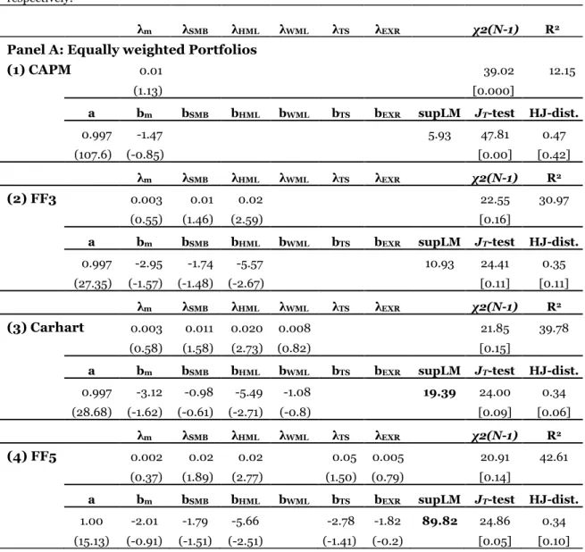
Table 2 Unconditional estimations with Fama-MacBeth (1973) and SDF-GMM regressions
The Table reports Fama-MacBeth (1973) price of risk estimations and factor sensitivities using the SDF-GMM methodology for the sample period from July, 1994 till May, 2009. The Table is divided into two panels.. Each panel is further divided into 4 distinct parts to report the corresponding factor premiums λj
and SDF factor sensitivities bj for (1) CAPM, (2) FF3, (3) Carhart and (4) FF5 models respectively. The
t-values for the estimates from both regressions are given in (). The first two rows of each partition provide the FM based factor risk premiums and t-values computable from the time series of cross-sectional estimates in the 2nd stage FM regressions. The χ2 (N-1) statistic and the average R2 are presented as
performance measures for the FM regressions. The χ2 statistic is distributed with N-1 degrees of freedoms
tests if the cross-sectional pricing errors are jointly zero. The 5th and 6th row in the partition present the
parameters of the respective model SDF with GMM t-values. The Andrews (1993) parameter stability test, Hansen (1982) over identification test and the Hansen and Jagannathan (1997) distance specification measures for the SDF-GMM estimations are notated with supLM, JT-test and δHJ. The significant supLM
test statistics at 5% critical values as given in the Andrews (1993) Table 1 are presented in bold. The p-values for the null hypothesis δHJ=0 are calibrated with Jagannathan and Wang (1996) simulation method.
The small/large p-values against/for the null hypotheses are given in [] for the noted test statistics respectively.
λm λSMB λHML λWML λTS λEXR χ2(N-1) R2 Panel A: Equally weighted Portfolios
(1) CAPM 0.01 39.02 12.15
(1.13) [0.000]
a bm bSMB bHML bWML bTS bEXR supLM JT-test HJ-dist.
0.997 -1.47 5.93 47.81 0.47
(107.6) (-0.85) [0.00] [0.42]
λm λSMB λHML λWML λTS λEXR χ2(N-1) R2
(2) FF3 0.003 0.01 0.02 22.55 30.97
(0.55) (1.46) (2.59) [0.16]
a bm bSMB bHML bWML bTS bEXR supLM JT-test HJ-dist.
0.997 -2.95 -1.74 -5.57 10.93 24.41 0.35
(27.35) (-1.57) (-1.48) (-2.67) [0.11] [0.11]
λm λSMB λHML λWML λTS λEXR χ2(N-1) R2
(3) Carhart 0.003 0.011 0.020 0.008 21.85 39.78
(0.58) (1.58) (2.73) (0.82) [0.15]
a bm bSMB bHML bWML bTS bEXR supLM JT-test HJ-dist.
0.997 -3.12 -0.98 -5.49 -1.08 19.39 24.00 0.34 (28.68) (-1.62) (-0.61) (-2.71) (-0.8) [0.09] [0.06]
λm λSMB λHML λWML λTS λEXR χ2(N-1) R2
(4) FF5 0.002 0.02 0.02 0.05 0.005 20.91 42.61
(0.37) (1.89) (2.77) (1.50) (0.79) [0.14]
a bm bSMB bHML bWML bTS bEXR supLM JT-test HJ-dist.
1.00 -2.01 -1.79 -5.66 -2.78 -1.82 89.82 24.86 0.34 (15.13) (-0.91) (-1.51) (-2.51) (-1.41) (-0.2) [0.05] [0.10]
12
Table 2 (Continued)
λm λSMB λHML λWML λTS λEXR χ2(N-1) R2 Panel A: Value weighted Portfolios
(1) CAPM 0.01 20.40 14.51
(1.75) [0.37]
a bm bSMB bHML bWML bTS bEXR supLM JT-test HJ-dist.
0.997 -3.79 16.95 30.61 0.34
(41.77) (-2.19) [0.04] [0.71]
λm λSMB λHML λWML λTS λEXR χ2(N-1) R2
(2) FF3 0.01 0.01 -0.001 15.33 35.50
(2.39) (1.55) (0.14) [0.57] []
a bm bSMB bHML bWML bTS bEXR supLM JT-test HJ-dist.
0.997 -4.59 -1.80 -1.49 26.92 21.76 0.29 (30.98) (-2.47) (-1.75) (-0.86) [0.19] [0.27]
λm λSMB λHML λWML λTS λEXR χ2(N-1) R2
(3) Carhart 0.014 0.01 -0.000 0.01 13.09 43.09
(2.52) (1.34) (-0.04) (1.61) [0.67]
a bm bSMB bHML bWML bTS bEXR supLM JT-test HJ-dist.
0.997 -4.82 -0.95 -1.52 -1.45 54.38 16.78 0.27 (29.25) (-2.53) (-1.65) (-0.93) (-1.33) [0.40] [0.31]
λm λSMB λHML λWML λTS λEXR χ2(N-1) R2
(4) FF5 0.01 0.01 -0.001 0.03 0.002 15.14 44.73
(0.54) (1.61) (-0.14) (1.11) (0.34) [0.44]
a bm bSMB bHML bWML bTS bEXR supLM JT-test HJ-dist.
0.997 -4.37 -1.69 -1.51 -0.79 -1.56 213.49 21.17 0.29 (26.44) (-2.1) (-1.57) (-0.83) (-0.3) (0.17) [0.13] [0.17]
Vaihekoski (2004) described low average dispersion across size portfolios, different to results in this study. The non-conformity could be owing to different sample periods or due to inclusion of delisted stocks. The most compelling reason for the observational differences is the use of logarithmic returns in his work rather than the simple relative returns used in this study. The continuously compounded returns are not linearly additive across the portfolio components, which is a well-reported drawback (Campbell, Lo, & Mackinlay, 1997).8
8 Campbell, Lo, and Mackinlay (1997) noted that this issue is minor at shorter time horizons, such as
daily time intervals. However, the portfolio returns calculated with log returns are downwardly biased in the range of 0.5 percent to 1.5 percent per month on average from the reported size-BM and industry
13
We further estimate the significance in the difference of means between the EW and VW portfolios by the t-test.9 The significant differences show that both the portfolios constructed
with alternating weighing schemes follow independent return paths overtime. The statistical significance of the difference in mean returns strengthens our expectation to look for specification errors of APM using EW and VW portfolios separately, given the peculiar market dynamics.
4. Estimations and Discussion 4.1. Unconditional models
The results for the unconditional models using EW portfolios are presented in panel A of Table 4. The work horse SDF estimations display the negative correlation of the market factor with the pricing kernel, which, in theory, is positively compensated risk. However, the estimates suffer from large sampling errors, and the 𝜒2-test rejects the null. The specification has highest HJ-distance and the parameter stability test rejects the null at 5 percent critical values. The value factor remains persistent in affecting the SDF and commanding a positive premium across FF3 and Crahart specification for EW test portfolios. The estimates for remaining risk factors are theoretically plausible however insignificant. The fit of the Carhart model is boosted with stable model parameters, least HJ pricing errors among the unconditional models. Furthermore, the FF3 specification among multi factor specifications suffers from parameter instability.
We augment the FF3 model with the term structure of interest rates and exchange rate risk, and label it FF5. The specification has smallest HJ-distance (34 percent) comparable to that of the Carhart model and has the highest R2 with stable model parameters. The results with VW
portfolios (Table 4 panel B) and the important divergence than the estimations using EW test portfolios is non-prevalence of the value factor and significance of market factor which affects
portfolios. The bias implies that logarithmic returns underreport the gains and over-report the losses of the constituent stocks in the respective portfolios.
9Following an anonymous referee, we pooled the stock data from New Zealand, Hong Kong and the
Netherlands and create 10 EW and VW size portfolios. Simple differences in means show stark dissimilarities in the returns of small and high capitalization portfolios than their EW counterparts. The t-statistic for the differences in mean is t-statistically different from zero for 7 out of 10 size portfolios. Unreported results are available upon request.
14
the pricing kernel and commands a significant risk premium across all the unconditional models. Moreover, the size factor influences in the FF3 model and is borderline significant at 10 percent in FF% specification, whereas the momentum remain unable to relate with the model SDF. Furthermore, the macro factors remain trivial for the VW portfolios.
The dissimilarity in evidence displays the differences in the returns generating processes for the average firm effect (EW) and the fate of invested capital respectively (VW). Such that average firm effect is better explained by value factor, but growth in inveted wealth is better explained by the market factor. Nevertheless, for capitalized portfolios, the CAPM is still unable to suppress cross-sectional mispricing, unlike the portfolio-based models.
4.2. Conditional CAPM
Hodrick and Zhang (2001) noted that the conditional models are attractive for surrogating the time varying risk premiums that are otherwise unavailable with the unconditional testing. However, the conditional tests more often suffer from parameter stability and for employing additional degrees of freedom (Ghysels, 1998). The model parameters increase geometrically with the number of conditioning variables. Therefore, given the small sample we condition only the single factor CAPM specification.
The SDF-GMM and price of risk estimations for the EW and VW portfolios are presented in Table 5 and Table 6 respectively. The role of scaling variables is to improve the misspecification of the unconditional CAPM compared to the competing multi-factor models. Generally, the joint zero mispricing null for the FM regressions is rejected across all the specifications except for the illiquidity-scaled CAPM as is shown in Table 5. Moreover, the estimate for the market beta risk is always positive yet insignificant. The first instrument used for the conditional CAPM specification is TS. The results suggest the term structure scaled model does not suppress the cross-sectional mispricing and so does a EXR scaled CAPM model. Important results are such that the DY scaled model has a R2 value comparable to that of
FF3 model and the positive compensation with increasing PER provides predictions contrary to conventional wisdom (Campbell & Shiller, 1988).
15
The price of risk estimations using January dummy show a large R2 value compared to the
FF3 model, but the January dummy neither influences the pricing kernel nor reduces the Table 3 Fama-MacBeth (1973) and Conditional SDF-GMM regressions (I)
The Table reports the conditional CAPM estimations for the EW portfolios with Fama-MacBeth (1973) procedure and SDF-GMM regressions during the sample from July, 1994 till May, 2009. The Table is divided into 9 sub panels. Each panel is numbered under heading IV-CAPM, where IV is the instrument variable used for the condition the unconditional CAPM. The factor risk premiums λIV, λm, and λIV.m, are
the premiums for the conditioning variables, market factor and interaction term of both respectively for the scaling variable as labeled in each sub panel. Similarly, the estimates under bIV, bm, and bIV.m manifest
the SDF factor sensitivities in the corresponding scaled CAPM specification. The t-values for the estimates from both regressions are given in ().The first two rows of each partition provide the FM based factor risk premiums and t-values computable from the time series of cross-sectional estimates in the 2nd stage FM
regressions. The χ2 (N-1) statistic and the average R2 are presented as performance measures for the FM
regressions. The χ2 statistic is distributed with N-1 degrees of freedoms tests if the cross-sectional pricing
errors are jointly zero. The 5th and 6th row in the sub panel present the parameters of the respective model
SDF with GMM t-values respectively. The Andrews (1993) parameter stability test, Hansen (1982) over identification test and the Hansen and Jagannathan (1997) distance specification measures for the SDF-GMM estimations are notated with supLM, JT-test and δHJ. The supLM test failing to reject the null
hypothesis of no structural shifts in the model parameters are presented in bold with the tabulated p-values in Andrews (1993) Table 1. The p-p-values for the null hypothesis δHJ=0 are calibrated with
Jagannathan and Wang (1996) simulation method. The small/large p-values against/for the null hypotheses are given in [] for the noted test statistics respectively.
λTS λm λTS.m χ2(N-1) R2
(1) TS-CAPM 0.02 0.004 0.01 36.93 27.3
(0.54) (0.51) (1.47) [0.00]
a bTS bm bTS.m supLM JT-test HJ-dist.
1.03 -3.07 -0.54 -25.21 47.31 47.16 0.45
(15.75) (-1.36) (-0.30) (-0.81) [0.00] [0.05]
λEXR λm λEXR.m χ2(N-1) R2
(2) EXR-CAPM 0.000 0.004 -0.001 28.28 28.42
(-0.02) (0.61) (-2.13) [0.04]
a bEXR bm bEXR.m supLM JT-test HJ-dist.
1.02 9.83 0.04 258.54 1252.80 33.94 0.40
(20.43 (0.81) (0.02) (2.05) [0.01] [0.14]
λLGB λm λLGB.m χ2(N-1) R2
(3) DY-CAPM -0.001 0.002 -0.004 36.79 29.27
(-1.58) (0.32) (0.41) [0.00]
a bDY bm bDY.m supLM JT-test HJ-dist.
1.00 247.60 -1.59 -925.75 32.34 47.47 0.45
(17.99) (0.84) (-0.80) (-0.42) [0.00] [0.03]
λPER λm λPER.m χ2(N-1) R2
(4) PER-CAPM 0.003 0.001 0.000 38.16 28.34
(1.22) (0.22) (0.34) [0.00]
a bPER bm bPER.m supLM JT-test HJ-dist.
1.00 1.53 -1.19 -138.36 27.05 34.70 0.46
16
Table 3 (Continued)
λJan λm λJan χ2(N-1) R2
(5) Jan.-CAPM 0.02 0.00 0.01 37.36 31.17
(0.32) (0.57) (1.35) [0.00]
a bJan bm bJan.m supLM JT-test HJ-dist.
1.02 -0.08 -0.70 -7.22 4.98 46.02 0.46
(20.97) (-0.12) (-0.40) (-1.12) [0.00] [0.01]
λILLIQ λm λILLIQ.m χ2(N-1) R2
(6) ILLIQ-CAPM 0.04 0.01 -0.001 22.14 30.24
(1.45) (1.59) (-1.90) [0.18]
a bILLIQ bm bILLIQ.m supLM JT-test HJ-dist.
1.07 -10.56 -4.78 168.25 9.45 19.44 0.35
(10.88) (-1.36) (-1.51) (1.96) [0.30] [0.39]
mispricing. Moreover, the SDF-GMM estimation suffers from parameter instability. Assuming 𝐼𝐿𝐿𝐼𝑄𝑚,𝑡as the expected market illiquidity, the positive premium highlights an overall compensation for bearing the average state of market illiquidity, although it is insignificant.10
The interaction term between market factor and expected illiquidity is negative and is significant with conventional t-values. The illiquidity scaled CAPM performs well for the EW portfolios and has the lowest 𝛿𝐻𝐽 among the scaled specifications however suffers from parameter instability as indicated by the Andrews (1993) supLM test.
The model parameters are stable for the conditional CAPM specifications using VW portfolios except for the PER scaled specification, as reported in Table 6. The other notable generalization is the significance of premia on market beta risk across all the scaled market model specifications, contrary to the evidence in Table 5. The simplifications for the scaled CAPM are consistent with the estimations of the unconditional models using VW test assets.
The TS-CAPM significantly prices the term structure risk and the interaction term. The significance of the term premium highlights that investors demand higher returns on stocks for positive increases in the TS. However, the term risk factor does not affect the pricing kernel
10 We assume lagged 𝐼𝐿𝐿𝐼𝑄
𝑚 as the expected market liquidity for its high persistence to generalize explanations for the expected state of market illiquidity.
17
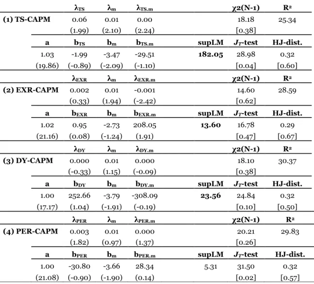
Table 4 Fama-MacBeth (1973) and Conditional SDF-GMM regressions (II)
The Table reports the conditional CAPM estimations for the EW portfolios with Fama-MacBeth (1973) procedure and SDF-GMM regressions during the sample from July, 1994 till May, 2009. The Table is divided into 9 sub panels. Each panel is numbered under heading IV-CAPM, where IV is the instrument variable used for the condition the unconditional CAPM. The factor risk premiums λIV, λm, and λIV.m, are
the premiums for the conditioning variables, market factor and interaction term of both respectively for the scaling variable as labeled in each sub panel. Similarly, the estimates under bIV, bm, and bIV.m manifest
the SDF factor sensitivities in the corresponding scaled CAPM specification. The t-values for the estimates from both regressions are given in ().The first two rows of each partition provide the FM based factor risk premiums and t-values computable from the time series of cross-sectional estimates in the 2nd stage FM
regressions. The χ2 (N-1) statistic and the average R2 are presented as performance measures for the FM
regressions. The χ2 statistic is distributed with N-1 degrees of freedoms tests if the cross-sectional pricing
errors are jointly zero. The 5th and 6th row in the sub panel present the parameters of the respective model
SDF with GMM t-values respectively. The Andrews (1993) parameter stability test, Hansen (1982) over identification test and the Hansen and Jagannathan (1997) distance specification measures for the SDF-GMM estimations are notated with supLM, JT-test and δHJ. The supLM test failing to reject the null
hypothesis of no structural shifts in the model parameters are presented in bold with the tabulated p-values in Andrews (1993) Table 1. The p-p-values for the null hypothesis δHJ=0 are calibrated with
Jagannathan and Wang (1996) simulation method. The small/large p-values against/for the null hypotheses are given in [] for the noted test statistics respectively.
λTS λm λTS.m χ2(N-1) R2
(1) TS-CAPM 0.06 0.01 0.00 18.18 25.34
(1.99) (2.10) (2.24) [0.38]
a bTS bm bTS.m supLM JT-test HJ-dist.
1.03 -1.99 -3.47 -29.51 182.05 28.98 0.32
(19.86) (-0.89) (-2.09) (-1.10) [0.04] [0.60]
λEXR λm λEXR.m χ2(N-1) R2
(2) EXR-CAPM 0.002 0.01 -0.001 14.60 28.59
(0.33) (1.94) (-2.42) [0.62]
a bEXR bm bEXR.m supLM JT-test HJ-dist.
1.02 0.95 -2.73 208.05 13.60 16.78 0.29
(21.16) (0.08) (-1.24) (1.91) [0.47] [0.67]
λDY λm λDY.m χ2(N-1) R2
(3) DY-CAPM 0.000 0.01 0.000 18.10 30.37
(-0.33) (1.15) (-0.09) [0.38]
a bDY bm bDY.m supLM JT-test HJ-dist.
1.00 252.66 -3.79 -308.09 23.56 24.84 0.32
(17.17) (1.04) (-1.91) (-0.19) [0.10] [0.50]
λPER λm λPER.m χ2(N-1) R2
(4) PER-CAPM 0.003 0.01 0.000 20.21 29.83
(1.82) (0.97) (1.37) [0.26]
a bPER bm bPER.m supLM JT-test HJ-dist.
1.00 -30.80 -3.66 28.34 5.31 31.50 0.32
18
Table 4 Continued
λJan λm λJan.m χ2(N-1) R2
(5) Jan.-CAPM 0.14 0.01 0.01 13.35 30.56
(2.22) (2.03) (1.61) [0.71]
a bJan bm bJan.m supLM JT-test HJ-dist.
1.13 -1.54 -3.20 -0.42 41.53 16.35 0.27
(19.60) (-2.40) (-1.62) (-0.05) [0.50] [0.84]
λILLIQ λm λILLIQ.m χ2(N-1) R2
(6) ILLIQ-CAPM 0.01 0.02 -0.0003 15.70 29.04
(0.41) (2.87) (-0.50) [0.55]
a bILLIQ bm bILLIQ.m supLM JT-test HJ-dist.
1.04 2.98 -4.43 87.84 65.12 19.13 0.30
(21.05) (0.49) (-2.24) (1.66) [0.32] [0.76]
significantly and have higher HJ distance. The scaled model with exchange rate changes explains larger variations in the VW portfolio returns than the EW counterpart. The price for euro/dollar fluctuations is positive yet insignificant. The result shows (implicitly) large capitalization Finnish firms are better hedged against currency fluctuations than the EW portfolios of small size firms. Importantly, the exchange rate-scaled specification has marginally lower HJ distance than the FF3 model and is second only to the Carhart model for the VW portfolios. The specifications with DY and PER are not attractive enough to affect the capitalized portfolio returns.
The most compelling performance is documented for the January-scaled CAPM using the VW portfolios. The estimations document a difference in the premiums for the month of January and the other months of the year. The evidence is consistent with Heston et al. (1999) for the European stocks. However, the implications are not similar to the U.S. market, as reported in Denial and Titman (1997), because the higher returns in January display more correspondence to the large capitalization stocks (the short side of size effect) than the BM effect. Importantly, the specification reduces the mispricing to similar levels, as with the best performing Carhart model. The results for ‘January effect’ from the Finnish market are contrary to the US evidence: using EW test portfolios (the best chance for value stocks, and small size
19
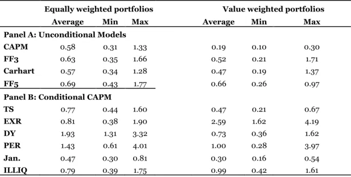
Table 5 Dynamic Model Performances
Table reports the results from linear projections of the pricing errors 𝛼̂𝑖,𝑡+1= 𝑀𝑡+1(𝑏̂)𝑅𝑖,𝑡+1onto a
set of conditioning vector 𝑧𝑡= (𝑇𝑆 𝐸𝑋𝑅 𝐷𝑌 𝑃𝐸𝑅 𝐼𝐿𝐿𝐼𝑄)′ as proposed by Farnsworth et al. (2002).
The model SDF,𝑀𝑡+1(), series is calculated using the one step SDF-GMM parametric solutions, 𝑏̂,
used in the estimation of HJ-distance measure. 𝑇𝑆 is the lagged difference between long rate series
and one month EURIBOR series, 𝐸𝑋𝑅 is the change in euro against USD at time 𝑡 and 𝐷𝑌 is the
aggregated market dividend yield. The 𝑃𝐸𝑅 is the price to earnings ratio for the market index and
𝐼𝐿𝐿𝐼𝑄 is aggregated market’s price impact to the euro volume traded. The Farnsowrth et al. (2002) diagnostic estimates of fitted pricing errors are presented under panel A and B respectively. The
first vertical partition of the Table presents the results using EW portfolios and the 2nd half with the
VW portfolios. The average standard deviation of projected pricing errors along with the minimum and maximum estimates using 20 excess portfolio returns and risk free rate proxy are given against each model tagged row. The lower average shows a particular model performs better in capturing the time series variability of asset returns in comparison to the results reported for other tested models.
Equally weighted portfolios Value weighted portfolios
Average Min Max Average Min Max
Panel A: Unconditional Models
CAPM 0.58 0.31 1.33 0.19 0.10 0.30
FF3 0.63 0.35 1.66 0.52 0.21 1.71
Carhart 0.57 0.34 1.28 0.47 0.19 1.37
FF5 0.69 0.43 1.77 0.66 0.26 0.97
Panel B: Conditional CAPM
TS 0.77 0.44 1.60 0.47 0.21 0.67 EXR 0.81 0.38 1.90 2.59 1.62 4.19 DY 1.93 1.31 3.32 0.73 0.36 1.62 PER 1.43 0.61 4.01 1.00 0.28 3.97 Jan. 0.47 0.30 0.81 0.30 0.16 0.54 ILLIQ 0.79 0.39 1.75 0.99 0.42 1.61
stocks) January dummy does not influence model SDF. However, for VW test portfolios the January dummy influences SDF. The lagged illiquidity interaction with market factor significantly influences the pricing kernel at 10 percent critical values, as shown in the Table 5. The over identification test statistic has large p- values and is unable to reject the null. However, the model is comparable to better performing models in terms of HJ-distance, if not the best.
Overall, the estimations for the VW portfolio highlight the fact that the market factor is persistent in influencing the specification pricing kernels with plausible risk compensations. Besides the implicit significance of the January effect for large capitalization firms, other important factor risks include EXR and ILLIQ-scaled market factors for both EW and VW
20
Table 6 Factor combinations based likelihood-ratio test
Table reports the Cochrane (1996) based likelihood ratio statistic establishing given an unrestricted model factors f1, are a restricted model factors f2 important for pricing assets. The LR test simplifies the idea if the restricted factors are not important for asset pricing then the GMM based minimized objective function 𝐽𝑇 compared to corresponding 𝐽𝑇estimate for the general model should not rise much. In order to employ the χ2-difference test we augment each model (excluding FF3) factors with the Fama and French (1993) model
risk factors, i.e., SMB and HML. Then we compare the performance of the augmented model with the restricted model that the regression estimates for SMB and HML are zero. The listed models in the column 1 of the Table represent the restricted model. Panel A reports the statistic for unconditional models for both EW and VW models in separate vertical partitions. Similarly, the performance of the conditioning variables is analyzed in Panel B. All the GMM estimations are done using general model weighting matrix. The significant increases in the restricted model minimized objective function show the restricted model factors outperform the SMB and HML factors or vice a versa. The test statistic is chi-square distributed with 2 (# of restrictions) degrees of freedom.
Equally weighted portfolios Value weighted portfolios
χ2(2) p-value χ2(2) p-value
Panel A: Unconditional Models
CAPM 23.40 0.00 8.86 0.01 Carhart 21.21 0.00 1.95 0.19 FF5 16.50 0.00 7.40 0.01
Panel B: Conditional CAPM
TS 23.24 0.00 8.80 0.01 EXR 11.65 0.00 1.38 0.25 DY 24.78 0.00 5.29 0.04 PER 13.44 0.00 8.03 0.01 Jan. 21.57 0.00 1.83 0.20 ILLIQ 0.65 0.36 3.30 0.10
portfolios. The results show that the misspecification of the static CAPM can be improved if the parameters of the scaled SDF are allowed to vary through time. However, the scaled CAPM specifications usually fail to capture the average tendency of the firms, except for the illiquidity-scaled CAPM. The dismal performance of the conditional-CAPM for EW portfolios highlights the lowness of conditioning variables in the predictability regressions (Table 3). However, the employed information variables performed much better for the capitalized portfolios, compared to the EW portfolios, in suppressing cross-sectional mispricing. Moreover, the varying risk explanations and differences in HJ-distances emphasize the otherwise shortcoming of generalized evidence for markets such as Finland.
21
4.3. Additional tests
In order to test the stability of the SDF-GMM estimations, we perform additional diagnostic tests. The first robustness test focuses on the time series predictability of the spreads on the test assets as proposed by Farnsworth et al. (2002). The results for the dynamic model performance are reported in Table 5. The linear projections show that the January-scaled CAPM is most successful in capturing the time variations in EW portfolio returns among all the tested specifications, followed by the Carhart model and the unconditional CAPM. The second diagnostic checks if a set of factors are important for pricing assets compared to another set of risk factors. Hansen’s (1982) 𝐽𝑇 statistic rejects the null hypothesis against a nonspecific alternative. Cochrane (1996) suggested testing a model against a specific alternative and proposed a likelihood-ratio (LR) test.
The LR test (Table 6) for EW portfolio returns shows that all the nested models are rejected against the pricing ability of the SMB and HML, excluding the ILLIQ-CAPM specification. The significance of the test statistic is highly robust (1 percent level) for the restricted unconditional and conditional specifications. The results with the LR test shows SMB and HML drives away the unsuccessful model SDF, except the ones that have fared well in suppressing the cross-sectional mispricing and therefore report the stability of the results in the sections 4.1 and 4.2. We also estimate all the models, excluding industry portfolios for robustness: the main evidence remains consistent (results available upon request).
5. Conclusions
This study accounts for the peculiar characteristics of small stock markets in analyzing the specification errors of asset-pricing models. Stock markets such as Finland are severely affected by carrying proportionally large capitalizations weights from one or a few firms and/or a small number of listed stocks. We hypothesize that because of the peculiar structure of small markets, the usual evidence with VW or EW portfolios will lack the overall picture for the economic wide risks. The horse race specification error testing among the tested APM for the Finnish
22
market follows Hodrick and Zhang (2001) and Schrimpf et al. (2008) for the U.S. and the German stock markets respectively. Furthermore, the results in the study pass a far stricter test for using different characteristic portfolios as suggested by Lewellen et al. (2010) in the related literature.
We report that performance of the unconditional CAPM specification could be improved if the parameters of the SDF are allowed to vary through time using certain conditioning variables. The size and value risk significantly affect the pricing kernel for the EW portfolios, whereas for the value weighted test assets market factor influences the model SDF persistently. Overall, the Carhart model produces the lowest HJ-distance among all tested models for both types of weighted portfolios. Similar evidence in suppressing mispricing is also reported by the FF5 model and the Jan.-CAPM for EW and VW portfolios respectively. Additionally, the diagnostic checks consolidate the evidence for better performance of the Carhart model.
The diverging persistence of risks elucidates the need for accounting the average stock sensitivity (EW) and the overall growth in the invested wealth (VW) separately for a market like Finland. The empirical results show deviation in the significant risk factors becomes prevalent for using a simple technique of EW and VW test assets. We conclude the benchmark evidence from asset pricing test for these markets should not be taken for granted and more investigative caution should be adopted when analyzing what are the risks that underlie stochastic changes in the return generating processes for all the firms in the cross-section. The results highlight the need for specification error testing from independent financial markets to report the impact of varying dynamics at play in atypical markets.
REFERENCES
Amihud, Y., 2002. Illiquidity and stock returns: Cross-section and time-series effects, Journal of Financial Markets, 5, 31-56.
Andrews, D., 1993. Tests for parameter instability and structural change with unknown change point, Econometrica, Vol. 61, 1993, 821–856.
23
Berglund, T. and Knif, J., 1999, Accounting for the accuracy of beta estimates in CAPM tests on assets with time-varying risks, European Financial Management, 5, 29–42.
Campbell, J.Y., Lo, A.W., and MacKinlay, A. C., 1997. The Econometrics of financial markets, USA: Princeton University Press.
Campbell, J.Y., and Shiller, R.J., 1988. Stock prices, earnings and expected dividends, Journal of Finance, 43,661–676.
Carhart, M., 1997. On persistence of mutual fund performance, Journal of Finance, 52, 57–82. Cochrane, J.H., 1996. A cross-sectional test of an investment-based asset pricing model, Journal
of Political Economy, 104, 572–621.
Daniel, K. and Titman, S., 1997. Evidence on the characteristics of cross sectional variation in stock returns, Journal of Finance, Vol. 52, 1–33.
Durack, N., Durand, R. D. and Maller, R., 2004. A best choice among asset pricing models? The conditional CAPM in Australia, Accounting and Finance, Vol. 44, 139–162.
Fama, E.F., and French, K.R., 1993. Common risk factors in the returns on stocks and bonds, Journal of Financial Economics, 33, 3–56.
Fama, E.F., and French, K.R., 1992. The cross-section of expected stock returns, Journal of Finance, 47, 427–465.
Fama, E.F., and MacBeth, J.D., 1973, Risk, return and equilibrium: Empirical tests, The Journal of Political Economy, 81, 607–636.
Farnsworth, H., Ferson, W., Jackson, D. and Todd, S., 2002. Performance evaluation with stochastic discount factors, Journal of Business, 2002, 473–503.
Fletcher, J. and Kihanda, R. J., 2005. An examination of alternative CAPM-based models in UK stock returns, Journal of Banking and Finance, 29, 2995–3014.
Ghysels, E., 1998. On stable factor structures in the pricing of risk: do time-varying betas help or hurt?, Journal of Finance, 53, 549–573.
Hansen, L.P., 1982. Large sample properties of generalized method of moment estimators, Econometrica, 50, 1029–1054.
24
Hansen, L.P., Heaton, J., and Yaron, A., 1996. Finite-sample properties of some alternative GMM estimators, Journal of Business and Economic Statistics, 14, 262–280.
Hansen L.P., and Jagannathan R., 1997. Assessing specification errors in stochastic discount factor models, Journal of Finance, 52, 557–590.
Heston, S. L., Rouwenhorst, K. G. and Wessels, R. E., 1999. The role of beta and size in the cross-section of European stock returns’, European Financial Management, Vol. 5, 9– 27.
Hodrick, R. J. and Zhang, X., 2001. Evaluating the specification errors of asset pricing models, Journal of Financial Economics, 62, 327–376.
Ilmanen, M. and Keloharju, M., 1999. Shareownership in Finland, Finnish Journal of Business Economics, 48, 257–285.
Jagannathan, R. and Wang, Z., 1996. The conditional CAPM and the cross-section of expected returns, Journal of Finance, 51, 3–53.
Kan, R., and Robotti, C., 2008.Specification tests of asset pricing models using excess returns, Journal of Empirical Finance, 15, 816–838.
Lally, M., and Swidler, S., 2008. Betas, market weights and the cost of capital: The example of Nokia and small cap stocks on the Helsinki stock exchange, International Review of Financial Analysis, 17, 805–819.
Lewellen, J., Nagel, S. and Shanken, J., 2010. A skeptical appraisal of asset pricing tests Journal of Financial Economics, 96, 175–194.
Lettau, M., and Ludvigson, S., 2001. Resurrecting the (C) CAPM: a cross-sectional test when risk premia are time-varying, Journal of Political Economy, 109, 1238–1287.
Loughran, T., 1997. Book-to-market across firm size, exchange, and seasonality: is there an effect? Journal of Financial and Quantitative Analysis, 32, 249–268.
25
Pätäri, E.J., Leivo, T.H., and Honkapuro, J.V.S, 2010. Enhancement of value portfolio performance using data envelopment analysis, Studies in Economics and Finance, 27,223–246.
Schrimpf, A., Schröder, M and Stehle, R., 2007. Cross-sectional Tests of Conditional Asset Pricing Models: Evidence from the German Stock Market, European Financial Management, 13, 880–907.
Shanken, J., 1992. On the estimation of beta-pricing models, Review of Financial Studies, 5, 1– 33.
Vaihekoski, M., 2009. Pricing of liquidity risk: Empirical evidence from Finland, Applied Financial Economics, 19, 1547–1557.
Vaihekoski, M., 2004. Portfolio construction for tests of asset pricing models, Financial Markets, Institutions & Instruments, 13, 1–39.
Vassalou, M., 2003. News related to future GDP growth as a risk factor in equity returns, Journal of Financial Economics, 68, 47–73.
Virk, N.S., 2012. Stock returns and macro risks: Evidence from Finland, Research in International Business and Finance, 26, 47–66.