Development and Applications of Machine Learning
Methods for Hyperspectral Data
Felix M. Riese
Doctoral Thesis Karlsruhe, 2020
Development and Applications of
Machine Learning Methods for
Hyperspectral Data
Doctoral Thesis
for the fulfillment of the requirements for the academic degree
Doctor of Engineering (Dr.-Ing.)
Accepted by
the KIT Department of Civil Engineering, Geo and Environmental Studies of the Karlsruhe Institute of Technology (KIT)
Submitted by
Felix M. Riese
born in Stuttgart, Germany
Day of examination 19 May 2020
Main referee Prof. Dr.-Ing. habil. Stefan Hinz
Institute of Photogrammetry and Remote Sensing (IPF) Karlsruhe Institute of Technology (KIT)
Co-referee Prof. Dr. Jocelyn Chanussot
Grenoble Images Speech Signal and Control (GIPSA) Grenoble Institute of Technology (INP)
Felix M. Riese
Development and Applications of Machine Learning Methods for Hyperspectral Data
Doctoral Thesis
Day of examination: 19 May 2020 Referees:
Prof. Dr.-Ing. habil. Stefan Hinz Prof. Dr. Jocelyn Chanussot
Karlsruhe Institute of Technology (KIT)
Department of Civil Engineering, Geo and Environmental Studies Institute of Photogrammetry and Remote Sensing (IPF)
Kaiserstr. 12 76131 Karlsruhe
This document is licensed under a Creative Commons
Attribution-ShareAlike 4.0 International License (CC BY-SA 4.0), if not stated otherwise:
„
Stay hungry. Stay foolish.—Steve Jobs (Co-Founder of Apple Inc.)
Abstract
Hyperspectral remote sensing of the Earth relies on data from passive optical sensors that are mounted on platforms such as satellites and Unmanned Aerial Vehicles (UAVs). Hyperspectral data includes information to identify materials and to monitor environmental variables, such as soil texture, soil moisture, chlorophyll a, and land cover. Data analysis methods are necessary to retrieve information from hyperspectral data. One powerful tool in the analysis of hyperspectral data is Machine Learning (ML), a subset of Artificial Intelligence. ML models can solve non-linear correlations and are scalable on increasing dataset sizes. Every dataset and every ML estimation task brings new challenges that require innovative solutions. The aim of the studies presented in this thesis is the development and applications of ML methods on hyperspectral remote sensing data. These studies address the following three main challenges: (I) datasets with only a few labeled datapoints, (II) the limited potential of shallow ML approaches on hyperspectral data, and (III) the challenge of dataset shift between training and test dataset.
The studies on the challenge (I) result in the development and publication of a Self-Organizing Map (SOM) framework for unsupervised, supervised, and semi-supervised learning. The SOM is applied to a hyperspectral dataset in the (semi-)supervised regression of soil moisture, outperforming a Random For-est (RF) regressor. The SOM framework shows adequate performance in the (semi-)supervised classification of land cover. It provides additional visualization capabilities to improve the understanding of the underlying dataset. In the studies addressing the challenge (II), three innovative 1-dimensional Convolutional Neural Network (CNN) architectures are developed. The CNNs are applied in the context of a soil texture classification to a freely available hyperspectral dataset. Their performance is compared with two existing CNN approaches and a RF classifier. Two main findings can be summarized. Firstly, the CNN approaches show significantly better performance than the applied shallow approach RF. Secondly, adding the information about hyperspectral band numbers to the input layer of a CNN improves the performance on the individual classes. The studies on the challenge (III) are based on a UAV dataset, acquired on five different measurement areas in Peru in 2019. Dataset shift is detected with qualitative methods and with unsupervised ML approaches, such as Principal Component Analysis and Autoencoder. Based
on the results, a supervised regression of soil moisture is performed on different combinations of measurement areas. Additionally, to study the effects of dataset shift on the regression, the dataset is augmented with Monte Carlo methods. The applied SOM regressor is relatively robust against soil moisture sensor noise and performs well on small datasets, while the applied RF performs best on the full dataset. Dataset shift makes this regression task difficult; some combinations of measurement areas form a significantly better training dataset than others. To conclude, the presented studies tackling the three main challenges show promising results. The developed ML methods can be further enhanced in future research.
Zusammenfassung
Die hyperspektrale Fernerkundung der Erde stützt sich auf Daten passiver optischer Sensoren, die auf Plattformen wie Satelliten und unbemannten Luftfahrzeugen montiert sind. Hyperspektrale Daten umfassen Informationen zur Identifizierung von Materialien und zur Überwachung von Umweltvariablen wie Bodentextur, Bo-denfeuchte, Chlorophyllaund Landbedeckung. Methoden zur Datenanalyse sind erforderlich, um Informationen aus hyperspektralen Daten zu erhalten. Ein leis-tungsstarkes Werkzeug bei der Analyse von Hyperspektraldaten ist das Maschinelle Lernen, eine Untergruppe von Künstlicher Intelligenz. Maschinelle Lernverfahren können nichtlineare Korrelationen lösen und sind bei steigenden Datenmengen skalierbar. Jeder Datensatz und jedes maschinelle Lernverfahren bringt neue Heraus-forderungen mit sich, die innovative Lösungen erfordern. Das Ziel dieser Arbeit ist die Entwicklung und Anwendung von maschinellen Lernverfahren auf hyperspektra-le Fernerkundungsdaten. Im Rahmen dieser Arbeit werden Studien vorgestellt, die sich mit drei wesentlichen Herausforderungen befassen: (I) Datensätze, welche nur wenige Datenpunkte mit dazugehörigen Ausgabedaten enthalten, (II) das begrenzte Potential von nicht-tiefen maschinellen Lernverfahren auf hyperspektralen Daten und (III) Unterschiede zwischen den Verteilungen der Trainings- und Testdatensätzen. Die Studien zur Herausforderung (I) führen zur Entwicklung und Veröffentlichung eines Frameworks von Selbstorganisierten Karten (SOMs) für unüberwachtes, über-wachtes und teilüberüber-wachtes Lernen. Die SOM wird auf einen hyperspektralen Datensatz in der (teil-)überwachten Regression der Bodenfeuchte angewendet und übertrifft ein Standardverfahren des maschinellen Lernens. Das SOM-Framework zeigt eine angemessene Leistung in der (teil-)überwachten Klassifikation der Land-bedeckung. Es bietet zusätzliche Visualisierungsmöglichkeiten, um das Verständnis des zugrunde liegenden Datensatzes zu verbessern. In den Studien, die sich mit Her-ausforderung (II) befassen, werden drei innovative eindimensionale Convolutional Neural Network (CNN) Architekturen entwickelt. Die CNNs werden für eine Boden-texturklassifikation auf einen frei verfügbaren hyperspektralen Datensatz angewen-det. Ihre Leistung wird mit zwei bestehenden CNN-Ansätzen und einem Random Forest verglichen. Die beiden wichtigsten Erkenntnisse lassen sich wie folgt zu-sammenfassen: Erstens zeigen die CNN-Ansätze eine deutlich bessere Leistung als der angewandte nicht-tiefe Random Forest-Ansatz. Zweitens verbessert das
Hinzu-fügen von Informationen über hyperspektrale Bandnummern zur Eingabeschicht eines CNNs die Leistung im Bezug auf die einzelnen Klassen. Die Studien über die Herausforderung (III) basieren auf einem Datensatz, der auf fünf verschiedenen Messgebieten in Peru im Jahr 2019 erfasst wurde. Die Unterschiede zwischen den Messgebieten werden mit qualitativen Methoden und mit unüberwachten maschinel-len Lernverfahren, wie zum Beispiel Principal Component Analysis und Autoencoder, analysiert. Basierend auf den Ergebnissen wird eine überwachte Regression der Bodenfeuchte bei verschiedenen Kombinationen von Messgebieten durchgeführt. Zusätzlich wird der Datensatz mit Monte-Carlo-Methoden ergänzt, um die Auswir-kungen der Verschiebung der Verteilungen des Datensatzes auf die Regression zu untersuchen. Der angewandte SOM-Regressor ist relativ robust gegenüber dem Rau-schen des Bodenfeuchtesensors und zeigt eine gute Leistung bei kleinen Datensätzen, während der angewandte Random Forest auf dem gesamten Datensatz am besten funktioniert. Die Verschiebung der Verteilungen macht diese Regressionsaufgabe schwierig; einige Kombinationen von Messgebieten bilden einen deutlich sinnvolle-ren Trainingsdatensatz als andere. Insgesamt zeigen die vorgestellten Studien, die sich mit den drei größten Herausforderungen befassen, vielversprechende Ergebnis-se. Die Arbeit gibt schließlich Hinweise darauf, wie die entwickelten maschinellen Lernverfahren in der zukünftigen Forschung weiter verbessert werden können.
Acknowledgement
I am writing and handing in this thesis during the time of the Coronavirus disease in 2019 and 2020. I am thankful for the people in the health system and in jobs of systemic importance who contribute towards stopping this crisis.
I am deeply grateful for the three very intense Ph.D. years. I feel lucky to be surrounded by so many inspiring and supportive people that I was able to meet along the way. While this thesis is my work, my research would not have been possible without the people I met. I can not acknowledge every person that has inspired and supported me during my Ph.D., but I will mention the most significant ones. First of all, I want to thank Stefan Hinz for supervising my Ph.D. at the Institute of Photogrammetry and Remote Sensing (IPF) of the Karlsruhe Institute of Technology (KIT), for giving me the freedom to pursue my research interests, and for being an absolute enabler. Stefan enabled me to give talks at different international conferences, to participate in the open-source community, and to spend time abroad on different occasions. These learning opportunities are truly valuable.
Secondly, I want to thank Sina Keller for being my direct supervisor. She invested countless hours discussing research and giving feedback. Sina inspired me with her strong drive and motivation to publish our research, and she was in charge of the TRUST project’s acquisition and management. Thanks to Sina, I changed my field of research and started my research at the IPF, which turned out to be a great experience. Sina resolved many blockers that came up during my Ph.D.; and with her help, I already had data within the first month of my Ph.D. to start my initial research. I have been fortunate to have Sina as my supervisor!
Thirdly, I want to thank my direct office colleagues Johanna Guth, Philipp Maier, and Tobias Guth, from the IPF. The combination of deep focus, intense discussions, and relaxed coffee breaks on our balcony made me enjoy my time at the institute even more. Furthermore, I thank Chris Michel for the useful discussions and his feedback on my research. I want to thank Jens Leitloff for keeping each other up-to-date with Machine Learning research, for his critical feedback on my research, for his outside-the-box ideas, and for our two shared talks at the PyCon and the M3 conference.
I am grateful for the opportunity to go to Australia and visit the company FluroSat in Sydney. The Graduate School for Climate and Environment (GRACE) at the KIT, with Andreas Schenk and Ilse Engelmann, funded my stay abroad and several external trainings. I thank Anastasia Volkova, the CEO of FluroSat, for heapsof amazing experiences I made during my visit. Further, I thank Juan Delard de Rigoulières Mantelli, Victor Proto, Leandro Giovannini, Thomas Sauvajon, and the whole team. Next, I want to thank Jocelyn Chanussot for being my co-referee, despite his incredi-ble workload and the external circumstances. I thank Heike Birkel for the perfect administrative support over the three years. Special thanks to Sven Wursthorn, who kept the IPF infrastructure running and the servers working around the clock. The successful measurement campaign in Peru would not have been successful without Samuel Schroers, Philipp Wagner, and Julian Bocanegra.
The work of this thesis benefited a lot from open-source software. I am thankful for the developers, for example, of Python, Python packages such as scikit-learn,
pandas, NumPy, matplotlib, as well as LATEX.
I want to thank my colleagues and friends from the Collège des Ingénieurs. Namely, I thank Elmar Mitterreiter and Florian Schäfer for their motivating support and their feedback on my research. Furthermore, I want to thank my friends for their support during my Bachelor’s, Master’s, and Ph.D. in Karlsruhe for mak-ing this time unforgettable. Special thanks to Timothy Gebhard and Carl De-gitz for their feedback on my research.
I am grateful for the unlimited support of my parents Susanne and Matthias Riese, and my sister Annika Riese.
I thank my partner Teresa for her support and her humor. Meeting her was a big highlight of my three Ph.D. years.
Thank you! Merci! Gracias! Grazie! Obrigado! Cheers mates! Danke!
Felix M. Riese Karlsruhe, June 2020
Contents
1 Introduction 1
1.1 Background . . . 1
1.2 Challenges and Overall Aim . . . 2
1.3 Outline and Main Contributions . . . 3
2 Hyperspectral Estimation Framework 7 2.1 Introduction . . . 7 2.2 Fundamentals . . . 8 2.3 Target Variables . . . 11 2.4 Sensor Level . . . 13 2.5 Data Level . . . 17 2.6 Feature Level . . . 22 2.7 Model Level . . . 25
2.8 Summary, Applications, and Extension . . . 36
3 Semi-Supervised Self-Organizing Maps for Regression and Classification 39 3.1 Introduction . . . 39
3.2 Related Work . . . 41
3.3 Unsupervised SOMs for Clustering . . . 43
3.4 Supervised SOMs for Regression and Classification . . . 48
3.5 Semi-Supervised SOMs for Regression and Classification . . . 52
3.6 Soil Moisture Regression . . . 53
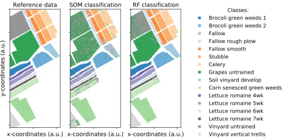
3.7 Land Cover Classification . . . 57
3.8 Conclusions and Outlook . . . 68
4 1D Convolutional Neural Networks for Hyperspectral Data 71 4.1 Introduction . . . 71
4.2 Related Work . . . 72
4.3 The LUCAS Soil Dataset . . . 74
4.4 Supervised Classification Models . . . 76
4.5 Results . . . 79
4.6 Discussion . . . 81
5 Dataset Shift in Hyperspectral Regression 85
5.1 Introduction . . . 85
5.2 Related Work . . . 86
5.3 The ALPACA Dataset . . . 87
5.4 Detection of Dataset Shift . . . 93
5.5 Effects of Dataset Shift on Supervised Regression . . . 100
5.6 Conclusions and Outlook . . . 108
6 Conclusions and Outlook 111 6.1 Conclusions . . . 111
6.2 Enhancements and Outlook . . . 116
Bibliography 117 List of Abbreviations 137 List of Figures 139 List of Tables 141 A List of Publications 143 B Variable Naming Conventions 147 C Supplementary Material 149 C.1 Supplementary Material of Chapter 3 . . . 149
C.2 Supplementary Material of Chapter 4 . . . 151
Introduction
1
„
Prediction, not narration, is the real test of ourunderstanding of the world.
—Nassim Nicholas Taleb (Statistician, Author)
1.1
Background
Vision is of utmost importance for humans. The human eye covers the electromag-netic spectrum from about 380 nm to 750 nm, referred to as the Visible Spectrum (VIS), in three different types of retinal cells [1, 2, 3]. Each type of retinal cell corre-sponds to a specific spectral band, characterized by the mean wavelength and band-width. The combination of these three spectral bands enables humans to distinguish between millions of colors and, therefore, to differentiate visually between materials. Humans can recognize, for example, roads, grass, and bare soil from color and spatial patterns. They perceive roads asgrey, grass asgreen, and bare soil asbrown. The Red–Green–Blue (RGB) color model is an adaptation of the three-spectra model of the human eye. For example, the majority of today’s consumer-grade cameras are based on passive, optical RGB sensors. Hyperspectral sensors extend this color model and the human vision by (i) increasing the number of spectral bands from three to about 10 to 1000 bands, (ii) decreasing the width of the spectral bands to a few Nanometers, and (iii) extending the spectral range into the infrared spectrum [2]. Depending on the type of hyperspectral sensor, it covers the Visible and Near-Infrared (VNIR), Short-Wavelength Near-Infrared (SWIR), or Thermal Near-Infrared (TIR) spectrum. The increased amount of information about the electromagnetic spectrum, compared to human vision and RGB cameras, improves the identification and differentiation of materials and monitoring of physical processes.
Hyperspectral remote sensing of the Earth applies hyperspectral sensors from satel-lites, airplanes, and Unmanned Aerial Vehicles (UAVs) [4, 5]. With these platforms,
hyperspectral data can be acquired over large areas and in short time scales. Hy-perspectral remote sensing derives information about, for example, soil texture and soil moisture, chlorophyllaconcentrations in inland waters, and changes in land cover and vegetation classes [6, 7, 8, 9]. This large variety of possible applica-tions makes hyperspectral remote sensing a valuable tool in many research fields of environmental sciences such as hydrology, ecology, and geology [2, 10]. In hyperspectral remote sensing, technological advances of the last decades have significantly lowered the costs of data acquisition with satellites and UAVs [11]. These technological advances have substantially increased computing power and data storage capabilities (big data). The resulting growth of data availability re-quires scalable data analysis tools. The increased computing power makes it pos-sible for Machine Learning (ML), which is a subset of Artificial Intelligence (AI), to become a standard data analysis tool in many research fields such as hyper-spectral remote sensing [10, 12, 13, 14, 15, 16].
ML methods can perform tasks such as supervised classification and regression with non-linear correlations [17]. For these tasks, ML models are built based on given training datasets consisting of input data and labels. The ML model learns patterns in the dataset. The aim in ML estimation is to train a ML model that generalizes to new input data. This means that the ML estimation can infer meaningful outputs between untrained input data or test datasets [18]. In the example of soil moisture regression from hyperspectral data, a hyperspectral image of a measurement area is the input data. The labels, referred to as ground truth or reference data, can be in situ soil moisture measurements.
1.2
Challenges and Overall Aim
This thesis focuses on ML estimations, such as the previous example of soil moisture regression from hyperspectral data. During several field experiments, heterogeneous datasets are acquired on different scales, in different countries, and with different hyperspectral sensors. Every dataset and every corresponding estimation task brings along new challenges that require new innovative, methodological solutions [10]. Three main challenges are the focus of this thesis:
(I) ML model training on datasets with only a few labeled datapoints,
(II) the limited potential of shallow ML approaches on hyperspectral data, and (III) the challenge of distribution differences between training and test dataset.
The overall aim of this thesis is to improve the quality of ML estimations based on hyperspectral data. This aim is achieved by (a) developing ML methods for hyper-spectral data to address the three main challenges, (b) applying innovative methods in current ML research to the field of hyperspectral remote sensing, and (c) providing these datasets, software, and evaluation scripts freely accessible to everyone.
1.3
Outline and Main Contributions
In the following, the structure of this thesis is outlined, and the main contribu-tions in every chapter are summarized. Figure 1.1 illustrates an overview of the structure, divided into six chapters and an appendix. Appendix A lists all pub-lications published within the scope of this thesis.
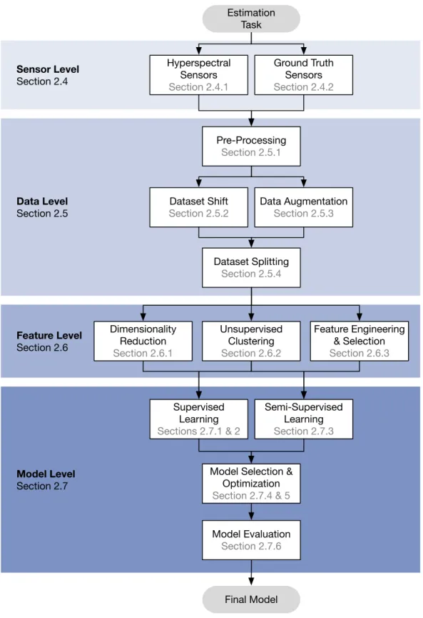
Chapter 2 – Framework The full range of the ML estimation based on hyperspec-tral data is presented as a hyperspechyperspec-tral estimation framework. The framework structures the process from a given estimation task to the final estimation in four levels. (i) The sensor level describes the acquisition of hyperspectral data and corresponding ground truth point data. (ii) The data level covers pre-processing, the challenge of dataset shift, data augmentation, and dataset splitting. (iii) The feature level includes the unsupervised dimensionality reduction, unsupervised clustering, feature engineering as well as feature selection. (iv) The model level consists of supervised learning, semi-supervised learning, model selection, the optimization of hyperparameters, and model evaluation metrics. The hyperspectral estimation framework is presented in Chapter 2. Each challenge is tackled with the presented framework and with strategies presented in Chapters 3 to 5.
Chapter 3 – Challenge (I) The acquisition of hyperspectral remote sensing data with modern satellite and UAV technology is getting increasingly affordable over large areas [19]. At the same time, the acquisition of reference data is still expensive in time and resources. Therefore, datasets often include significantly more hyper-spectral data than reference data. Both hyperhyper-spectral data and reference data are needed for proper training of ML models. This is the first challenge addressed in this thesis. In Chapter 3, a framework of Self-Organizing Maps (SOMs) is introduced as a semi-supervised ML approach. SOMs are underrepresented in today’s research [20]. This chapter fills this gap with the following four main contributions:
• the publication of a hyperspectral field campaign dataset,
• the development and publication of a (semi-)supervised SOM framework, • the application of this framework in the regression of soil moisture, and
• the application of this framework in the classification of land cover.
Chapter 4 – Challenge (II) The second challenge is the limited potential of shallow ML models on high dimensional data. Shallow learners such as Random Forest and Support Vector Machine show adequate performance in hyperspectral applications. They often depend on feature engineering or dimensionality reduction, which adds inductive bias. Inductive bias can support the generalization of the ML model but also limit its potential [21]. Deep learning approaches, such as Convolutional Neural Networks (CNNs), are one solution for this challenge. In the field of hyperspectral remote sensing, CNNs are mostly applied on 2-dimensional (2D) images rather than on 1-dimensional (1D) spectra. The studies presented in Chapter 4 fill this gap in hyperspectral remote sensing research with the following two main contributions:
• the development and publication of deep 1D CNN architectures, and • the application of these models on an existing soil texture dataset.
Chapter 5 – Challenge (III) The third challenge is dataset shift in hyperspectral datasets. In general, dataset shift occurs if the distributions of the input data and labels of a training dataset differ from the distributions of a test dataset. A consequence of dataset shift for ML estimation is the ability to generalize to new input data [22]. Dataset shift is a common challenge in ML research and hy-perspectral remote sensing, but researchers mostly ignore it. Chapter 5 fills this gap with the following four main contributions:
• the publication of a hyperspectral UAV dataset,
• the detection of dataset shift with unsupervised ML approaches, • the development of a data augmentation method, and
• the study of the effects of dataset shift on supervised soil moisture regression.
Chapter 6 – Conclusions and Outlook The findings of this thesis are summarized in Chapter 6. The conclusion is followed by an outlook of extensions of the pre-sented studies and proposed future studies.
Chapter 1 Challenges of ML estimation
with hyperspectral data (I)
ML model training on datasets with a few
labeled datapoints (II) Limited potential of shallow ML models on hyperspectral data (III) Dataset shift in hyperspectral datasets Chapter 2
Hyperspectral Estimation Framework
Chapter 3 Semi-Supervised Self-Organizing Maps Chapter 4 1D Convolutional Neural Networks Chapter 5 Detection and Effects
of Dataset Shift
Chapter 6 Conclusions and Outlook
Figure 1.1: Overview of the logical structure of this thesis. In Chapter 1, three main
challenges are introduced in the estimation based on hyperspectral data. A hyperspectral estimation framework is the basis for the subsequent studies and is described in Chapter 2. Three studies are presented which address the three main challenges in Chapters 3 to 5. A conclusion of results and an outlook is given in Chapter 6.
Hyperspectral Estimation
Framework
2
„
The signal is the truth. The noise is whatdistracts us from the truth.
—Nate Silver (Statistician, Political Forecaster)
This chapter includes material from
Felix M. Riese and Sina Keller. “Supervised, Semi-Supervised, and Unsu-pervised Learning for Hyperspectral Regression”. In: Hyperspectral
Im-age Analysis: Advances in Machine Learning and Signal Processing. Ed. by
Saurabh Prasad and Jocelyn Chanussot. Cham: Springer International Publishing, 2020. Chap. 7, pp. 187–232. Reprinted with permission. It is cited as [7] andmarked in blue.
2.1
Introduction
Hyperspectral data, in general, requires different handling compared to other data when applying Machine Learning (ML). Hyperspectral data is high-dimensional, its spectral bands can be highly correlated, and the amount of ground truth for supervised estimation tasks is often small. In this chapter, a hyperspectral estimation framework is introduced, which covers the ML estimation based on hyperspectral data from the data acquisition to the final estimation. The focus lies on data-driven ML models since they are capable of dealing with non-linear estimation tasks (e.g. [23]). The terms hyperspectral regressionandhyperspectral classificationare introduced for the regression or classification solely based on hyperspectral data. The structure of this chapter is illustrated in Figure 2.1. At first, the fundamentals of hyperspectral regression and classification with different learning techniques and definitions of technical terms are presented in Section 2.2. The target variables
for the ML estimations, applied in this thesis, are described in Section 2.3. After the fundamentals, the four levels of the framework are introduced: sensor level, data level, feature level, and model level. On the sensor level in Section 2.4, hyperspectral data is combined with ground truth. The data level in Section 2.5 is structured into four parts: pre-processing, dataset shift, data augmentation, and dataset splitting. This level is followed by the feature level in Section 2.6, divided into dimensionality reduction, clustering, and feature engineering, as well as feature selection. The fourth level is the model level in Section 2.7. Two supervised models are presented, semi-supervised learning is summarized, and the model selection, optimization as well as evaluation are addressed.
2.2
Fundamentals
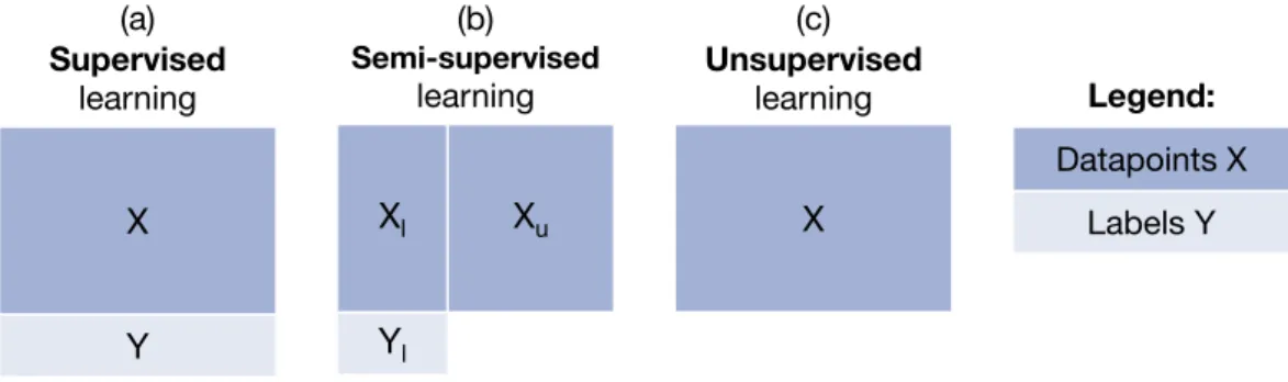
In recent years, the hyperspectral remote sensing community mainly focused on clas-sification tasks. Clasclas-sification refers to the estimation of discrete classes, for example, to distinguish between land cover classes likewater,vegetation,road, andbuilding. Both classification and regression are about building predictive models. The differ-ence is that, in classification, the target space is discrete (e.g., land cover classes), whereas in regression, the targets are continuous (e.g., soil moisture). [7, Sec. 7.2] In the context of ML regression, different approaches can be applied depending on the objective and the availability of reference data. In Figure 2.2, these different approaches are visualized schematically. We can distinguish [... three] cases. In case (a), reference data, meaning labels containing the ground truth, is available for all (hyperspectral) input datapoints. In this context, supervised learning models are suitable. A supervised model is able to learn from all available input-output data pairs. In case (b), we have an incompletely labeled dataset. That is, some of the samples are missing the correct ground truth labels. In this context, we can rely on semi-supervised learning models. They learn from the complete input-output pairs as well as from the datapoints without labels. [...] Finally, in the case (c) when no labels are available, unsupervised learning can be applied. Unsupervised learning is useful, for example, for dimensionality reduction and clustering. [7, Sec. 7.2] The mathematical notation conventions used in this chapter are consistent with [24] [and are listed in Table B.1]: X = (x1,. . .xn) is a set of n input datapoints xi ∈ X for all i∈[n] := {1,. . .n}. Every datapoint xi consists of m input features. In hyperspectral regression [and classification], the input features represent the m hyperspectral bands and it is X ⊂ Rm. In supervised learning, case (a), yi ∈ Y
Model Level Section 2.7 Supervised Learning Sections 2.7.1 & 2 Semi-Supervised Learning Section 2.7.3 Model Selection &
Optimization Section 2.7.4 & 5 Model Evaluation Section 2.7.6 Feature Level Section 2.6 Dimensionality Reduction Section 2.6.1 Unsupervised Clustering Section 2.6.2 Feature Engineering & Selection Section 2.6.3 Final Model Data Level Section 2.5 Pre-Processing Section 2.5.1 Dataset Shift Section 2.5.2 Dataset Splitting Section 2.5.4 Sensor Level Section 2.4 Hyperspectral Sensors Section 2.4.1 Ground Truth Sensors Section 2.4.2 Estimation Task Data Augmentation Section 2.5.3
Figure 2.1: Hyperspectral estimation framework divided into the sensor level, the data
X Y Xl Yl Xu (a) Supervised learning (c) Unsupervised learning (b) Semi-supervised learning X Datapoints X Labels Y Legend:
Figure 2.2: Depending on the availability of labels for our training data, we can distinguish
three types of learning algorithms: (a) supervised learning, (b) semi-supervised learning, and (c) unsupervised learning. (adapted with permission from [7])
with Y = (y1,. . ., yn) are the labels of the datapoints xi and the training set is given as pairs (xi, yi). In semi-supervised and active learning, cases (b) and (c), the dataset X is divided into two parts. The first part consists of the datapoints Xl := (x1,. . ., xl) with the corresponding labels Yl := (y1,. . ., yl) and the second parts consists of the datapoints Xu := (xl+1,. . ., xl+u) without any labels. It is l + u = n. Again, we have yi ∈ Y for i = 1,. . ., l. For regression, the labels are continuous in the cases (a) to (c) which meansY ⊂ R. Note that also
more-dimensional labels can be used in regression. In the d-more-dimensional case, it is Y ⊂ Rd. Within the scope of this chapter, we will stick to 1-dimensional (1D)
labels, meaning d = 1. [For classification, the labels are discrete in the cases (a) to (c).] We refer to this combination of hyperspectral input data and desired output data asdatapoint. In the unsupervised case (d), the dataset only consists of input datapoints X without any labels. [7, Sec. 7.2]
In the field of hyperspectral remote sensing and in the analysis of hyperspectral data, there are many applications for ML. [...] A general overview of remote sensing image processing with a focus on traditional ML models and physical models is given in [10]. Most current studies address ML classification with hyperspectral data (e.g., overview in [13]) whereas only few studies focus on hyperspectral regression (e.g., [5, 4]). The ML models used for the respective regression [and classification] tasks are described in Sections 2.7 and 2.7.3. [7, Sec. 7.2]
Depending on the hyperspectral regression [or classification] task, we need to select an appropriate ML model [17]. At best, the selected ML model is able to learn all relevant nuances of the training dataset (low bias) and is able to generalize well on unknown datasets (low variance). Accomplishing low bias and low variance at the same time is impossible. Thus, a trade-off between bias and variance [25, 26, 27] has to be addressed while selecting an appropriate model (see Section 2.7.4).
When an ML model is characterized by a low bias (high variance), it is able to adapt well to the training dataset which also includes noise. Such an ML model tends towards overfitting. An ML model with low variance is more robust against noise and outliers. Such an ML model is not able to adapt well to the nuances of the training dataset which is called underfitting. [7, Sec. 7.2]
2.3
Target Variables
The ML applications presented in this thesis focus on the estimation of three variables: soil moisture, soil texture, as well as land cover and land use. In the following, these three target variables are defined, and their relevance is described. Soil moisture is described in Section 2.3.1, soil texture is described in Section 2.3.2, and land cover and land use are described in Section 2.3.3.
2.3.1
Soil Moisture
Soil moisture is defined as the water contained in the part of the soil surface, which is unsaturated [28]. One measure of soil moisture is volumetric soil moisture, meaning the volume of water in a specific volume of soil. Therefore, soil moisture values are dimensionless and commonly provided in percentage. Soil moisture is an essential variable in hydrological, ecological, and climatological systems [28, 29]. Precise data about the soil moisture distribution helps in the modeling of these systems. In hydrology, the soil moisture dynamics of a river catchment gives a measure of the saturation of the soil. With the knowledge about the degree of soil saturation, the amount of infiltration and runoff from the water of a rainfall event, for example, can be estimated [28]. In climatology, soil moisture is a crucial variable in the global wa-ter and energy cycle since the wawa-ter and heat exchange between the Earth’s surface, and the atmosphere depends on the soil moisture [30]. In ecology and, especially, in ecosystems with limited water availability, knowledge about soil moisture helps in plant irrigation management, drought forecasting, and crop yield [31]. Soil moisture on the soil surface is spatially and temporally highly variable. The variability mainly depends on topography, soil texture, organic matter content, soil macroporosity, vegetation density and type, land use as well as climatologi-cal and meteorologiclimatologi-cal factors such as precipitation and solar radiation [32, 33, 28]. The water transmission and retention of the soil, for example, depends on
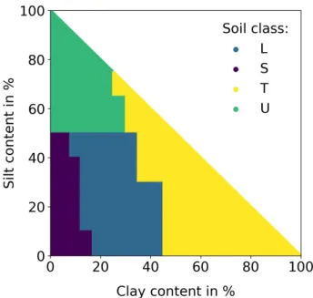
Figure 2.3: Main classes of soil texture according to Bodenkundliche Kartieranleitung ed. 5 (KA5): L (mainly loam), S (mainly sand), T (mainly clay), and U (mainly silt).
the soil texture: soils with larger particle sizes have a lower capacity to hold water than soils with smaller particle sizes [34].
2.3.2
Soil Texture
Soil is the composition of soil particles with various sizes. These soil parti-cles can be classified according to their diameters into clay (< 0.002 mm), silt (0.002 mm to 0.05 mm), and sand (0.05 mm to 2 mm). The relative content of clay, silt, and sand is referred to as soil texture. It can be classified, for example, according to the Bodenkundliche Kartieranleitung ed. 5 (KA5) taxonomy [35] or the United States Department of Agriculture (USDA) soil taxonomy [36]. Within the scope of this work, the KA5 taxonomy is used. The KA5 soil classes are listed in [35] with their clay, silt, and sand contents. Figure 2.3 illustrates the four KA5 main classes. Soil texture is a vital soil property for hydrology and agriculture [37, 38]. The ability to store water depends on the soil texture, which directly influences the availability of water for crops in agriculture. Smaller particle sizes, meaning a higher clay content, leads to higher water and nutrient holding capacity and to less oxygen. Overall, soil texture influences the soil response to environmen-tal conditions like droughts and rainfall.
2.3.3
Land Cover and Land Use
Land cover is defined as the material that covers the Earth’s surface. Examples for land cover classes areforest land,water, andwetland. Land use is the human’s use and modifications of the Earth’s surface. Exemplary land use classes arecropland,
orchards,residential buildings, andindustrial buildings. Since land cover and land
use classes overlap, both terms are used synonymously [39].
Changes in land cover significantly impact ecological systems; they affect global warming, erosion of soils, and biodiversity [40]. Further, information about changes in land cover and land use is essential for governments to monitor and manage countries and cities.
2.4
Sensor Level
For the estimation based on hyperspectral data, this data needs to be acquired with appropriate sensors. The first level of the presented hyperspectral estimation framework is, therefore, the sensor level. Datasets for the estimation of hyper-spectral data consist of data from a hyperhyper-spectral sensor and, depending on the application, of ground truth data. An overview of the hyperspectral sensors ap-plied in this work is presented in Section 2.4.1. The ground truth data is mostly acquired point-wise. In this work, the estimation of soil moisture, soil texture, and land cover is studied based on hyperspectral data. In Section 2.4.2, the most relevant measurement techniques are presented.
For the datasets used in this work, hyperspectral data and ground truth data are com-bined on different scales. In Chapter 3, the Karlsruhe Lysimeter (KarLy) soil moisture dataset on a small field scale is presented and applied [41, 42]. The Land Use/Cover Area Frame Survey (LUCAS) dataset is used in Section 4.3 for the estimation of soil texture [43, 44, 45]. This dataset includes data from soil samples all over Europe. The Aerial Peruvian Andes Campaign (ALPACA), introduced and used in Chapter 5, consists of hyperspectral Unmanned Aerial Vehicle (UAV) data combined with soil moisture in situ measurements on field scale. An additional dataset is used in further studies [46, 23, 47] for the estimation of soil moisture: the Field experiment dataset of surface-subsurface infiltration dynamics acquired by hydrological, remote sensing, and geophysical measurement techniques (HydReSGeo) [48].
2.4.1
Hyperspectral Sensors
Hyperspectral sensors are passive, optical sensors. These sensors are designed for their particular purposes and applications. Depending on the number of bands and the width of the bands, a sensor can be considered monospectral, multispec-tral, or hyperspectral. Sensors with one band are consideredmonospectral, sensors with approximately 2 to 15 relatively wide bands are considered multispectral, and sensors with approximately 100 to 1000 narrow bands are considered
hy-perspectral. Within the scope of this thesis, several different hyperspectral and
multispectral sensors are applied. The sensors are differentiated by the platform on which they are mounted, the spectral range, spectral resolution (number and width of bands) as well as the output type. The following platforms are consid-ered: a static tripod, a handheld sensor, UAV, airplane, and satellite. Additionally, hyperspectral sensors can be applied in a laboratory setup.
Three spectral ranges are considered: Visible and Near-Infrared (VNIR) from ap-proximately 400 nm to 1400 nm, Short-Wavelength Infrared (SWIR) from approx-imately 1400 nm to 3000 nm, and Thermal Infrared (TIR) from approxapprox-imately 3 µm to 15 µm. The output format of the sensors can be a single spectrum (spec-trometer), line data (line scanner), and images (snapshot). A qualitative overview of the four primary hyperspectral sensors applied in this work regarding the spatial, temporal, and spectral resolutions is shown in Figure 2.4. The spatial resolution refers to the sensor’s pixel size, the temporal resolution refers to the number of measurements that are possible during a specific time interval, and the spectral resolution refers to the number and width of the bands. The more bands and the smaller the width of the bands, the larger the spectral resolution gets. All applied sensors and their properties are listed in Table 2.1.
2.4.2
Ground Truth Measurements and Sensors
This work focuses on the estimation of soil moisture, soil texture, and land cover. The relevance of these variables is explained in Section 2.3. The ground truth of these variables comes from direct observation instead of inference. While the ground truth of land cover is generated manually by experts, the ground truth of soil moisture and soil texture requires specific sensors. This section provides an overview of mea-surement techniques for soil moisture and soil texture. In comparison to area-wide hyperspectral sensors, these ground truth measurements are performed point-wise.
T able 2.1 : Overview of the hyperspectral sensors applied within the scope of this thesis. Sensor name Sensor Sensor type Spectral range Number Own studies platform in nm of bands Hyperspectral Devices RO X T ripod Spectrometer 400 to 950 769 [9] Cubert UHD 285 T ripod Snapshot 450 to 950 125 Chapter 3 and (50 × 50 pixels) [42, 41, 23, 6, 7, 48, 49] ASD FieldSpec 4 Handheld Spectrometer 350 to 2500 2151 [46, 48, 49] FOSS XDS Rapid Content Analyzer Laboratory Spectrometer 400 to 2500 4200 Chapter 4 and [8] A VIRIS Airplane Line scanner 400 to 2500 224 Chapter 3 and [6] ESA Sentinel-2 Satellite Line scanner 420 to 2370 13 [50, 51] Headwall Hyperspec SWIR U A V Line scanner 900 to 2500 170 Chapter 5 FLIR T au 2 640 T ripod Snapshot 7500 to 13 500 1 [23, 52, 48] (640 × 512 pixels)
Spectral resolution Spatial resolution Temporal resolution Headwall Hyperspec SWIR Cubert UHD 285 Foss XDS Rapid Content Analyzer AVIRIS
Figure 2.4: Qualitative overview of the hyperspectral sensors mentioned in this work in
regards to the spatial, temporal and spectral resolutions.
Soil moisture can be measured, for example, point-wise with gravimetric meth-ods, with nuclear methmeth-ods, electromagnetic measurement techniques, tensiometer methods, and hygrometric methods [53]. The measurements are either performed directly at the measurement site (in situ) or performed indirectly by analyzing a soil sample in the laboratory. In contrast, area estimations are performed regionally on one area per measurement. Area estimations with remote sensing techniques can only measure soil moisture of the upper few centimeters of the soil. A more detailed overview of soil moisture estimation from remote sensing can be found in [54]. Since every soil moisture measurement technique comes with its limitations, there is not a single superior measurement technique [55]. In the following, the gravimetric method, are described as well as the two electromagnetic measurement techniques, which are applied in the presented studies in Chapters 3 and 5: Time Domain Reflectometry (TDR) sensors and capacitive sensors.
Gravimetric methods are based on drying a soil sample in the laboratory. The weight of the soil sample before and after the drying process is measured. The difference of both weights refers to the water content in the soil sample and, therefore, to its soil moisture. This measurement technique is invasive since it requires a soil sample. Therefore, it is mostly used as a baseline and for the calibration of other methods. Electromagnetic measurement techniques for soil moisture include resistive sensors,
capacitive sensors, TDR sensors, and frequency domain sensors [55]. These meth-ods are based on the electromagnetic characteristics of water and, therefore, soil moisture. Capacitive sensors measure soil moisture by measuring the capacitance between electrodes in the soil. TDR sensors emit an electric pulse into an electrode located in the soil. The reflection of this pulse correlates with the soil moisture around the TDR sensor. TDR sensors are widely applied since they are non-invasive and easy to apply [56]. A quality assessment of TDR sensors is presented in [57]. Further details and other methods can be found in [28].
The soil texture of a soil sample can be determined with a laboratory method, re-ferred to as Particle Size Analysis (PSA) [58]. In the PSA, the different particle sizes within the soil sample are separated from each other. The resulting distribution can be used with a taxonomy such as the KA5 taxonomy [35] or USDA soil taxon-omy [36], as described in Section 2.3.2. This laboratory method is applied in the dataset used in the studies of Chapter 4, as described in [44, 43].
Land cover and land use ground truth can be acquired in a field survey, resulting in a land cover map. The exact classes have to be set beforehand. The number of different classes depends on the application of the dataset to be acquired.
2.5
Data Level
In the following, the data level as the second level of the presented hyperspec-tral estimation framework is described. The data level is divided into four parts: pre-processing, dataset shift, data augmentation, and dataset splitting. In Sec-tion 2.5.1, the pre-processing is described focusing on collecting, validating, and preparing the data. The second part of the data level addresses the challenges of dataset shift in Section 2.5.2. This includes possible approaches to cope with dataset shift. Data augmentation is presented in Section 2.5.3, including basic image manipulations, Monte Carlo (MC) augmentation, and Generative Adver-sarial Networks (GANs). The data level is concluded by several approaches of dataset splitting in Section 2.5.4. [7, Sec. 7.3]
2.5.1
Pre-Processing
The first part of the presented hyperspectral [... estimation framework] is pre-processing [10, 59]. We divide the pre-pre-processing into three steps: reading in data, preparing data, and validating data. First, we need to read in the data. In
Python, datasets can be conveniently read in using existing and established software packages such asPandas [60] or TensorFlow[61]. [7, Sec. 7.3.1]
The second step of pre-processing is the validation of the data. We highly recommend to explore the dataset before further processing [...]. The exploration procedure could include a check of the value range of the input features and the target variable. The data validation can be achieved by an analysis of the datasets statistics and by a visualization of the dataset. Thus, we obtain an overview of the used dataset. Additionally, we recognize possible challenges in the dataset such as outliers, missing values or labels as well as dataset shift at an early stage. The latter is addressed in detail in Section 2.5.2. A useful example to motivate the investigation of the dataset with statistical methods and visualizations is given in [62]. [7, Sec. 7.3.1] The last step of pre-processing is the preparation of the data. Depending on the results of the data validation and the applied ML models (see Sections 2.7 and 2.7.3), the dataset might need to be normalized or transformed. The data normalization makes the training less dependent on the scale of the input data. Typical nor-malization techniques scale the numerical data, for example, linearly between 0 and 1, or around 0 with a standard deviation of 1. Additionally, it might be neces-sary to transform categorical data to numerical values since some ML models like Artificial Neural Networks (ANNs) (see Section 2.7.2) only work with numerical data. A common way to achieve this isone hot encoding. Each categorical feature is represented by one entry in a binary vector. [7, Sec. 7.3.1]
2.5.2
Dataset Shift
Most ML models rely on the Independent and Identically Distributed (i.i.d.) as-sumption. The i.i.d. assumption refers to the independent collection of the training dataset and new, unknown datasets (see Section 2.5.4) which are identically distributed. [7, Sec. 7.3.2]
In this context, the term training dataset refers to the dataset that is available during the training of the ML model. For example, in hyperspectral regression of soil moisture, the hyperspectral data as well as the ground truth labels of soil moisture should cover all (in reality) possible values. Otherwise, dataset shift occurs and the estimation performance might suffer [22, 63]. In general, three main types of dataset shift exist: [7, Sec. 7.3.2]
• Covariate shift [64, 65] is defined as a change of the input feature distribution P(X). It is the best studied type of dataset shift in the literature. For exam-ple in hyperspectral regression of soil moisture, rainfall events between two measurement days affect the input feature distribution of this two-day dataset. • Prior probability shift [66, 63] is defined as a change of the target variable
distribution P(Y) without a change in X. This change mostly occurs in the application of generative models. For example, in the hyperspectral regression of soil moisture, the distribution of soil moisture can vary due to the underlying soil structure while the soil surface remains unchanged.
• Concept shift [67] or concept drift is a change in the relationship between the input data and the target variable. The concept shift is the most challenging type of dataset shift to handle. For example, in hyperspectral regression of chlorophyll a concentration, the relationship between hyperspectral input data and chlorophyll aconcentration as target variable can change due to undetectable hydrochemical processes. [...]
Several causes of dataset shift exist. One cause is the sample selection bias. Sample selection bias can occur in the scope of different data measurements. In hyperspectral regression [or classification], it often occurs as a result of the parallel use of different hyperspectral sensors and changes of the measuring site. Another cause for dataset shift [... are] non-stationary environments. Non-stationary environments appear when the training environment differs from the test environment. This distinction can be temporal or spatial. Since hyperspectral satellites record data at different locations and during different seasons, dataset shift commonly occurs. [7, Sec. 7.3.2] Various ways exist to deal with the challenges of dataset shift. In most ML stud-ies for hyperspectral regression [or classification], dataset shift is simply ignored. In this case, the applied model is static with regards to the dataset shift. Such models can be used further as a baseline model allowing the detection of dataset shift and enabling the evaluation of approaches aiming at the reduction of the effects of dataset shift. [7, Sec. 7.3.2]
A first approach to reduce the effects of dataset shift is to re-fit or update the ML model to new data. In the case of time series, this means re-fitting or up-dating the ML model on more recent data. In the case of 2-dimensional (2D) areal data, this means re-fitting on more training areas. Another approach is to re-weight the training dataset based on temporal (time series) or spatial (2D data) features. For example, training data of time series can be re-weighted so that newer datapoints are more important in the training than preceding ones.
Fur-ther, the ML model can be set up to inherently learn temporal changes to reduce the bias of seasonality and timing. [7, Sec. 7.3.2]
2.5.3
Data Augmentation
Limited dataset size, in general, is a challenge for ML models. Especially for deep architectures of ANNs and for estimations based Convolutional Neural Networks (CNNs), a large dataset size is crucial (see Section 2.7.2). Sensor uncertainties and noise are other challenges in the estimation based on hyperspectral data. In this section, three data augmentation approaches are presented: data augmentation with basic image manipulations, MC data augmentation, and GANs. An overview of data augmentation approaches in deep learning is presented in [18, 68]. Data augmentation with basic image manipulations includes flipping, rotating, and translation of images as well as color space transformations [68]. That way, one image of a dataset can be used several times in the training of a ML model. Current ML Python packages such asTensorFlow[61] already come with built-in image manipulation methods. In [69], the implementation of these manipulation methods is provided for multispectral satellite data.
Monte Carlo (MC) data augmentation is based on the generation of random samples according to distributions which depend on the experiment at hand. For example, a normal distribution of sensor uncertainty is often assumed to simulate sensor noise in the data augmentation. The normal distribution results from the central limit the-orem (e.g. [70]). The probability density for the normal distribution p(x) is defined, with the meanµand the varianceσ2 of the measured soil moisture values x, as
p(x) = √ 1 2πσ2exp – (x –µ)2 2σ2 ! . (2.1)
For MC data augmentation, the generation of pseudo data, a random data generator is needed. In general, it is recommended to apply existing, well-tested random data generators. Within the scope of this work, a random generator from the Python libraries SciPy and NumPy [71] is used, which is based on PCG64 [72]. In reference [47], the augmentation of soil moisture data from two sources is studied in the estimation of soil moisture from hyperspectral data. Two differ-ent MC augmdiffer-entation datasets, augmdiffer-entation over time and space, are included.
An overview of hyperspectral data augmentation is presented in [73]. MC data augmentation is applied in Section 5.5.1.
Generative Adversarial Networks (GANs) [74] are an upcoming ML model which was introduced for unsupervised data augmentation. GANs consist of two ANNs: a generator network and a discriminator network. The generator network learns to generate new data samples. In combination with the existing (real) training data, these new (fake) samples constitute the input data for the discriminator network. The discriminator network learns to differentiate between real and fake input data. During the training of a GAN, both networks learn to improve their performance re-garding their respective task. Finally, a trained GAN is able to generate new training data which can be used to augment the existing training dataset [...]. [7, Sec. 7.6.1] A detailed overview on GANs is presented in [75]. In hyperspectral regres-sion, GANs are not commonly used so far, although there are different ap-plications in classification. For example, the implementation of GANs and their applications on open hyperspectral classification datasets is presented in [76]. A more complex approach combining GANs with Semi-Supervised Learning (SSL) is presented in [77]. [7, Sec. 7.6.1]
2.5.4
Dataset Splitting
To evaluate the generalization abilities of an ML model, the full available dataset needs to be split into smaller datasets. In general, dataset splitting should meet the i.i.d. assumption (see Section 2.5.2). [... There are two commonly applied types of dataset splitting.] In the first type, the full dataset is split into two subsets:training
and test. In the second type, the three subsets training,validation, and test are generated. In both split types, the training dataset is used repeatedly to train the ML model. The test dataset is used only once to evaluate the final ML model. The split types differ with respect to the way the ML models are optimized (see Section 2.7.5). In the 3-subset split, the validation dataset is repeatedly used for the evaluation of the generalization abilities of the ML model in the optimization process. In the 2-subset split, the training dataset is used for both training and evaluation in the optimization process by applying a k-fold cross-validation. Within the k-fold cross-validation, the training dataset is randomly partitioned into k subsets of similar size. One of the k subsets is then used for the evaluation of the ML model, while the remaining k – 1 subsets are used for the training of the ML model. This selection is repeated so that every subset is used once as validation subset. Note that it is not trivial to apply k-fold cross-validation on time series due to possible casual relationships. [7, Sec. 7.3.3]
After deciding on the number of dataset subsets, the splitting approach needs to be defined. [...] They are described in detail in [78] with their respective strengths and weaknesses. The most commonly applied splitting approach is a random split or ran-dom sampling (e.g., [79]). The subsets are ranran-domly sampled which leads to subsets with relatively similar target variable distributions. However, for spatially or tem-porarily correlated data like 2D hyperspectral image data or time series, a pixel-wise random split can lead to biased subsets. Since a significant number of datapoints in one subset have direct spatial or temporal neighbors, the datapoints are highly cor-related in between the subsets. Training on one datapoint and evaluating the model performance on a neighboring datapoint leads to highly biased results. [7, Sec. 7.3.3] In [7], further splitting approaches are presented and discussed: systematic splitting, patch splitting and stratified splitting. Within the scope of this thesis, we rely on random splitting as discussed in the relevant sections.
2.6
Feature Level
The feature level is the third level of the presented hyperspectral estima-tion framework. It consists of unsupervised dimensionality reduction (Sec-tion 2.6.1), unsupervised clustering (Sec(Sec-tion 2.6.2), and feature engineering as well as feature selection (Section 2.6.3).
2.6.1
Dimensionality Reduction
Since correlations and redundancies between input features can occur, the virtual dimensionality of a dataset is often smaller than the given dimensionality [80]. The
termdimensionality reductionrefers to the reduction of the dimension m of the input
data to a smaller dimension mr≤m toward the virtual dimensionality. In addition, the termcompressionfocuses on the reduction of the dimension m of the data to the smallest possible mmin≤mr ≤m. In most cases after applying dimensionality reduction, it is only possible to reconstructsimilardata, not the original input data. The topic of dimensionality reduction and compression in general is reviewed in detail in [81, 82]. Note that the termfeature extraction is often used instead of dimensionality reduction (see e.g., [83]). [7, Sec. 7.4.1]
A more recent overview of dimensionality reduction approaches is presented in [16]. The authors provide an overview of state-of-the-art dimensionality reduction
proaches, divided into shallow and deep approaches. Overall, they compare 15 ap-proaches in terms of their impact on the accuracy of the exemplary classification task.
We discuss in the following the most relevant approaches of dimensionality reduction in hyperspectral regression [... and classification]. A commonly applied approach is the Principal Component Analysis (PCA) [84]. The PCA transforms the input data orthogonally based on the variance along newly found axes. These new axes are referred to as principal components. The principal components are sorted by decreas-ing variance. That is, the first principal component has the largest variance. There-fore, the set of the first few principal components contain most of a dataset’s variance and at best, most of the information contained in the dataset. [...] [7, Sec. 7.4.1]
Autoencoder (AE) [85] is an ANN approach for dimensionality reduction. An AE consists of an input layer of input dimension m, followed by several hidden layers with smaller dimension mhidden< m and an output layer of size m. The dimension reduction of input to hidden layers is calledencoding. In the encoding, the AE finds a lower-dimensional representation of the input data. The dimension increase of the encoded data in the original dimension m is calleddecoding. The AE is trained in an unsupervised manner with the hyperspectral data for both input and (desired) output data. Then, the encoding part of the trained AE can be used for dimensionality reduction on the (hyperspectral) input data. In sum, the full AE with encoding and decoding can also be used for noise removal (denoising) of the hyperspectral input data. More details about ANN are presented in Section 2.7.2. Since an AE consist of many free parameters, large training datasets are necessary for the training. Note that only the number of hyperspectral input datapoints needs to be large for the AE. The dataset that includes ground truth labels can be small. Since the combination of large input data and small ground truth data is characteristic for multi- and hyperspectral satellite data, AE is well-suited in this context. [...] [7, Sec. 7.4.1]
Finally, we list two additional dimensionality reduction approaches. The t-Distributed Stochastic Neighbor Embedding (t-SNE) [86] is a non-linear approach which reduces high-dimensional input data to a dataset with the dimension mr∈{2, 3}. Therefore, this approach is well suited not only for dimensionality reduction but for the visualiza-tion of a dataset as well. A recently presented dimensionality reducvisualiza-tion approach is called Uniform Manifold Approximation and Projection (UMAP) [87]. UMAP is com-parable with the t-SNE algorithm incorporating several advantages in terms of speed and performance. Since UMAP is a relatively new approach, it has to be investigated further in context of hyperspectral regression [and classification]. [7, Sec. 7.4.1]
2.6.2
Unsupervised Clustering
Clustering a dataset means the grouping datapoints with respect to a pre-defined similarity metric. Datapoints are clustered, mostly in an unsupervised manner, based on the input features such as hyperspectral bands.
The original publication [7] describes and compares the k-means clustering [88], the Density-Based Spatial Clustering of Applications with Noise (DBSCAN) al-gorithm [89], and unsupervised Self-Organizing Map (SOM) [90]. We omit this part because Chapter 3 introduces a framework of unsupervised, super-vised, and semi-supervised SOMs in detail [6].
2.6.3
Feature Engineering and Feature Selection
Feature Engineering In Sections 2.6.1 and 2.6.2, we apply dimensionality reduc-tion and clustering to generate new features. In contrast to these data-driven approaches, feature engineering is based on prior knowledge. The generated fea-tures can be categorized as spectral feafea-tures or spatial feafea-tures. The engineering of spectral features is inspired by physical processes. Spectral features are com-monly characterized by a ratio or the normalized difference of hyperspectral bands. The most popular example in hyperspectral regression [and classification] is the Normalized Difference Vegetation Index (NDVI) [91] which corresponds to pho-tosynthesis processes. Spatial features are often generated based on contextual information of neighboring pixels (datapoints). Examples for spatial features are objects, edges, and contours. They are generally created by the application of filters. Note that spatial features can only be generated [... for] hyperspectral images when their corresponding spatial resolution is adequate. [...] [7, Sec. 7.4.3]
In recent years, the application of (manual) feature engineering has decreased in hyperspectral regression [and classification]. Deep ANNs, which are able to learn new low-level and high-level features automatically (see Section 2.7.2), are the main reason for this development. Admittedly, incorporating domain knowledge into data-driven ML models might still improve their performance. Especially, the estimation of physical parameters in hyperspectral regression can be improved by including domain knowledge if such knowledge is available. An overview of the domain knowledge integration into ML models is given in [92] including a review and a consistent taxonomy on previous research. The authors distinguish between four possible approaches to include prior knowledge into ML models [92]: [7, Sec. 7.6.2]
• Integration of the knowledge into the training data by feature engineering (see Section 2.6.3) and simulations (see Section 2.5.3).
• Integration of the knowledge into the hypothesis space, for example by choos-ing an appropriate ML model such as CNNs for 2D hyperspectral data in the case of locality and translation invariance (see Section 2.7.2).
• Integration of the knowledge into the training algorithm, for example by modifying the loss function.
• Integration of the knowledge into the final hypothesis, for example by including physical constraints on the output variable.
Domain knowledge is included in a data-driven ML model, mainly to increase the model’s ability to generalize on new, unknown data. The domain knowledge itself adds a bias to the ML model, which is referred to asinductive bias(e.g. [21]).
Feature Selection In contrast to feature engineering, feature selection describes the process of selecting a subset of all available input features which can be used as input data for supervised ML models. In context of hyperspectral regression [and classifi-cation], the termband selectionis often used instead of the term feature selection. The main advantage of feature selection over feature engineering or dimensionality reduction is that the features (hyperspectral bands) are physically meaningful. For example, principal components can not be interpreted physically (see Section 2.6.1). Therefore, feature selection applied on data of one sensor can be transferred to data of another sensor with slightly different hyperspectral bands. [...] [7, Sec. 7.4.3] An overview of feature selection is presented in [93]. A review on several ap-plications of feature engineering and feature selection in the context of remote sensing image processing is provided in [10]. [...] The use of feature selec-tion and feature engineering depends on the dataset as well as on the applied supervised ML model. [7, Sec. 7.4.3]
2.7
Model Level
Hyperspectral regression and classification is based on mapping hyperspectral in-put data with desired outin-put data with a specific ML model. Two supervised ML approaches are presented in the following: tree-based models (Section 2.7.1) and ANNs (Section 2.7.2). An overview of semi-supervised learning based on hyper-spectral data is given in Section 2.7.3. The selection of an appropriate ML model
is addressed in Section 2.7.4, followed by the hyperparameter optimization (Sec-tion 2.7.5) and the model evalua(Sec-tion metrics (Sec(Sec-tion 2.7.6). This chapter is followed by Chapter 3, which is about a specific type of ML model, the supervised SOMs. Afterward, deep 1D CNNs are introduced and applied in Chapter 4.
2.7.1
Tree-based Models
Tree-based regression is based on Decision Trees (DTs). DTs consist of a root node and leave nodes connected by branches. The basic idea is to split the training dataset at every branch into subsets based on the input features, for example hyperspectral bands. In the best case, this split leads to leafs at the end of the branches containing similar values of the respective physical parameter to be estimated. The algorithm of DT regression is defined as follows [94] [7, Sec. 7.5.1.2]:
1. Start with the root node.
2. Start with the most significant input feature (hyperspectral band) of the training data, for example according to the Gini impurity.
3. Divide the input data with a (binary) cut c1 on that input feature xi, for example according to the Gini impurity.
4. Divide data along the next best feature on cut cjfor j = 2, 3,. . . which are calculated similarly to step 3.
5. Stop if a condition is met, for example, maximum number of nodes, maximum depth, or maximum purity.
6. Then, the ground truth labels of the datapoints are averaged for every individ-ual leaf. Finally, every leaf contains one output value.
DTs can also be applied for the classification of discrete target variables. The algorithm changes in step 6. The averaging of the ground truth labels over every individual leaf is replaced, for example, by a majority vote.
In the context of regression, the trained DT is applied for the estimation of the physical parameter. Every input datapoint is mapped onto a leaf containing the respective output value. In steps 2 and 4, the DT algorithm finds the most important feature at each branch in order to divide the dataset into more homogeneous subsets. For this reason, most software implementations of the DT algorithm return a trained estimator and an importance ranking of each input feature. This ranking is called feature importance. In the case of regression with hyperspectral data, the importance ranking refers to the hyperspectral bands. The implementation of the feature importance differs depending on the applied software. For example, the
feature importance can be based on the permutation of the respective values of each input feature. The bigger the influence of an input feature on the regression [or classification] performance, the more important it is. [7, Sec. 7.5.1.2]
[...] To address the issue of overfitting of a single DT, an ensemble of trees can be used. In the following, we focus on two ensembling techniques: bagging and boosting. The main idea of bootstrap aggregation, or bagging, is to average over a number of estimators trained on slightly different training datasets. In case of tree-based regression, the average is calculated over multiple DTs with different setups or training datasets. The trees are trained in parallel. Random Forest (RF) is one implementation of bagging with DTs [95]. Its algorithm is defined in the initialization (step 1) and three repeated steps (steps 2 to 4) [7, Sec. 7.5.1.2]:
1. Initialization: Set the number of trees B, the number of features is m.
2. Bootstrap: Sample learning batch containing n datapoints with replacement from a dataset with n datapoints. There should be n1 ≈ 2/3n different samples.
3. Feature bagging: At every node, a random subset of mbag = √m features are used for the splitting. This leads to a decreasing correlation between the different trees.
4. Regression [or classification]: See DT algorithm above.
Every tree only uses between 60 % to 70 % of the datapoints for the training process. The remaining 30 % to 40 % of the datapoints can be used to evalu-ate the estimation performance of the respective trees. The regression error of these trees on their ignored datapoints is called out-of-bag error and is a good estimate for the generalization error of the ML model. This reduces the need for an extra validation dataset. [7, Sec. 7.5.1.2]
Extremely Randomized Trees (ET) are a modification of the RF algorithm [96]. Compared to the RF algorithm, the splitting process for each node is modified. Randomized thresholds are calculated for each feature of the random subset. Finally, the best threshold is used for the split in the respective node. This modification leads to less variance and increases the bias [of the model]. [...] [7, Sec. 7.5.1.2] Boosting is another technique to improve the regression based on DTs [97, 98]. It relies on learning multiple estimators which are incrementally generated and improved. Gradient Tree Boosting (GTB) as an example of a boosting algorithm applies a gradient descent optimization [99, 100]. Shallow trees are fitted iteratively on the negative gradient of the loss function. [7, Sec. 7.5.1.2]


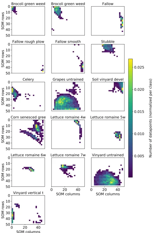
![Figure 3.7: Overview of the Salinas Airborne Visible Infrared Imaging Spectrometer (AVIRIS) dataset with 16 classes and a spatial resolution of 3.7 m [189]](https://thumb-us.123doks.com/thumbv2/123dok_us/9791530.2470949/72.892.241.632.106.416/overview-salinas-airborne-visible-infrared-imaging-spectrometer-resolution.webp)