Random Forest Algorithm for Land Cover Classification

Scholar Works at UT Tyler

Computer Science Faculty Publications and

Presentations

School of Technology (Computer Science &

Technology)

3-18-2016

Random Forest Algorithm for Land Cover

Classification

Arun D. Kulkarni

University of Texas at Tyler, [email protected]

Barrett Lowe

Follow this and additional works at:

https://scholarworks.uttyler.edu/compsci_fac

Part of the

Computer Sciences Commons

This Article is brought to you for free and open access by the School of Technology (Computer Science & Technology) at Scholar Works at UT Tyler. It has been accepted for inclusion in Computer Science Faculty Publications and Presentations by an authorized administrator of Scholar Works at UT Tyler. For more information, please [email protected].

Recommended Citation

Kulkarni, Arun D. and Lowe, Barrett, "Random Forest Algorithm for Land Cover Classification" (2016).Computer Science Faculty Publications and Presentations.Paper 1.

_______________________________________________________________________________________

Random Forest Algorithm for Land Cover Classification

Arun D. Kulkarni and Barrett Lowe

University of Texas at Tyler, Tyler, TX 75799, USA

[email protected]

Abstract— Since the launch of the first land observation satellite Landsat-1 in 1972, many machine learning algorithms have been used to classify pixels in Thematic Mapper (TM) imagery. Classification methods range from parametric supervised classification algorithms such as maximum likelihood, unsupervised algorithms such as ISODAT and k-means clustering to machine learning algorithms such as artificial neural, decision trees, support vector machines, and ensembles classifiers. Various ensemble classification algorithms have been proposed in recent years. Most widely used ensemble classification algorithm is Random Forest. The Random Forest classifier uses bootstrap aggregating for form an ensemble of classification and induction tree like tree classifiers.

A few researchers have used Random Forest for land cover analysis. However, the potential of Random Forest has not yet been fully explored by the remote sensing community. In this paper we compare classification accuracy of Random Forest with other commonly used algorithms such as the maximum likelihood, minimum distance, decision tree, neural network, and support vector machine classifiers.

Keywords- Random Forest, Induction Tree, Supervised Classifiers, Multispectral Imagery

__________________________________________________*****_________________________________________________

I. INTRODUCTION

Multispectral image classification has long attracted the attention of the remote-sensing community because classification results are the basis for many environmental and socioeconomic applications. Classification of pixels is an important step in analysis of Thematic Mapper (TM) imagery. Scientists and practitioners have made great efforts in developing advanced classification approaches and techniques for improving classification accuracy. However, classifying remotely sensed data into a thematic map remains a challenge because many factors, such as the complexity of the landscape in a study area, selected remotely sensed data, and image processing and classification approaches may affect the success of classification [1]. There are many methods to analyze Landsat TM imagery. These include parametric statistical methods or non-parametric soft computing techniques such as neural networks, fuzzy inference systems and fuzzy neural systems. Conventional statistical methods employed for classifying pixels in multispectral images include the maximum likelihood classifier, minimum distance classifier, and various clustering techniques. The maximum likelihood classifier assumes normal density functions for reflectance values and calculates the mean vector and covariance matrix for each class using training data sets. The classifier uses Bayes’ law to calculate posterior probabilities. In maximum likelihood classification, each pixel is tested for all possible classes and the pixel is assigned to the class with the highest posterior probability [2].

It is well established that neural networks are a powerful and reasonable alternative to conventional classifiers. Studies comparing neural network classifiers and conventional classifiers are available. Neural networks offer a greater degree of robustness and tolerance compared to conventional classifiers. With neural networks, once a neural network is trained it directly maps the input observation vector to the output category. Thus for large images neural networks are more suitable. Many researchers have used neural networks to classify pixels in multispectral images. Chen et. al [3] have

used dynamic learning neural networks for land cover classification of multispectral imagery. Foody [4] has used multi-layer perceptron (MLP) and Radial Basis Function Networks (RBN) for supervised classification. Huang and Lippmann [5] have compared neural networks with conventional classifiers. Eberlein et al. [6] have used neural network models for data analysis by a back-propagation (BP) learning algorithm in a geological classification system. Cleeremans et al. [7] have used neural network models with a BP learning algorithm for Thematic Mapper data analysis which was available on previous versions of Landsat. Decatur [8] has used neural networks for terrain classification. Kulkarni and Lulla [9] have developed three models: a three -layer feed forward network with back-propagation learning, a three-layer fuzzy-neural network model, and a four-layer fuzzy-neural network model. The models were used as supervised classifiers to classify pixels based on their spectral signatures. They considered two Landsat scenes. The first scene represents the Mississippi river bottomland area, and the second scene represents the Chernobyl area. Clustering algorithms such as the split-merge [10], fuzzy K-means [11], [12], and neural network based methods have been used for multispectral image analysis. Kulkarni and McCaslin [13] have used neural networks for classification of pixels in multispectral images and knowledge extraction.

Support vector machines (SVMs) is a supervised non-parametric statistical learning method. The SVM aims to find a hyper-plane that separates training samples into predefined number of classes [14]. In the simplest form, SVMs are binary classifiers that assigns the given test sample to one of the two possible classes. The SVM algorithm is extended to non-lineally separable classes by mapping samples in the feature space to a higher dimensional feature space using a kernel function. SVMs are particularly appealing in remote sensing field due to their ability to successfully handle small training datasets, often producing higher classification accuracy than traditional methods [15]. Mitra et al. [16] have used a SVM for classifying pixels in land use mapping.

_______________________________________________________________________________________

Decision trees represent another group of classification algorithms. Decision trees have not been used widely by the remote sensing community despite their non-parametric nature and their attractive properties of simplicity in handling the non-normal, non-homogeneous and noisy data. Hansen et al. [17] have suggested classification trees as an alternative to traditional land cover classifiers. Ghose et al. [18] have used decision trees for classifying pixels in IRS-1C/LISS III multispectral imagery, and have compared performance of the decision tree classifier with the maximum likelihood classifier.

More recently ensemble methods such as Random Forest have been suggested for land cover classification. The Random Forest algorithm has been used in many data mining applications, however, its potential is not fully explored for analyzing remotely sensed images. Random Forest is based on tree classifiers. Random Forest grows many classification trees. To classify a new feature vector, the input vector is classified with each of trees in the forest. Each tree gives a classification, and we say that the tree “votes” for that class. The forest chooses the classification having the most votes over all the trees in the forest. Among many advantages of Random Forest the significant ones are: unexcelled accuracy among current algorithms, efficient implementation on large data sets, and an easily saved structure for future use of pre-generated trees [19]. Gislason et al. [20] have used Random Forests for classification of multisource remote sensing and geographic data. The Random Forest approach should be of great interest for multisource classification since the approach is not only nonparametric but it also provides a way of estimating the importance of the individual variables in classification. In ensemble classification, several classifiers are trained and their results combined through a voting process. Many ensemble methods have been proposed. Most widely used such methods are boosting and bagging [18].

The outline of the paper is as follows. Section 2 describes decision trees and Random Forest algorithm. Section 3 provides implementation of Random Forest and examples of classification of pixels in multispectral images. We compare performance of the Random Forest algorithm with other classification algorithms such as the ID3 tree, neural networks, support vector machine, maximum likelihood, and minimum distance classifier. Section 4 provides discussion of the findings and concludes.

II. METHODOLOGY

A. Decision Tree Classifiers

Decision tree classifiers are more efficient than single-stage classifiers. With a decision tree classifier, decisions are made at multiple levels. Decision tree classifiers are also known as multi-level classifiers. The basic concerns in a decision tree classifier are the separation of groups at each non-terminal node and the choice of features that are most effective in separating the group of classes. In designing a decision tree classifier it is desirable to construct the optimum tree so as to achieve the highest possible classification accuracy with the minimum number of calculations. A binary tree classifier is considered a special case of a decision tree classifier. Appropriate splitting conditions vary among applications. A node is said to be a terminal node when it contains only one class decision. Three widely used methods in designing a tree are entropy, gini, and twoing. In the first method entropy is

used as a basic measure of the amount of information. The expected information needed to classify an observation vector D is given by:

 

 

log

Info D

p

p

 



where pi is the probability that an observation vector in D belongs to class Ci [21]. This is the most widely used splitting condition as it attempts to divide the classes as evenly as possible giving the most information gain between child and parent nodes. Some applications may require that the data be split by the largest homogeneous group possible. For this the gini information gain is used. Gini impurity is the probability that a randomly labelled class, taking into account class distribution and priors, is incorrectly labelled. Information gain using the gini index is defined as:

 



where pi is the probability that an observation vector in D belongs to class Ci . Another method used for splitting is twoing, which uses a different strategy to find the best split among cases [22]. It gives strategic splits by, at the top of the tree, grouping together classes that are largely similar in some characteristic. The bottom of the tree identifies individual classes. When twoing, classes are grouped into two super classes containing an as equal as possible number of cases. The best split of the super classes is found and used as the split at the current node. This results in a reduction of class possibilities among cases at each child node and a reduction in impurity. The splitting of data at each node is recursive and continues until a stopping condition is met. An ideal leaf node is one that contains only records of the same class. In practice reaching this leaf node may require an excessive number of splits that are costly. Splitting too much results in nothing more than a lookup table and will perform poorly for noisy data while splitting too little prevents error in training data from being reduced, increasing the error of the decision tree [23]. The decision to continue splitting can be based on previously mentioned information gain. The stopping condition could also be satisfied by thresholding the depth of children of a certain node. Another common method is to threshold the number of existing cases at the leaf node. If there are fewer cases than some threshold, splitting does not occur [18].

A variation of the basic decision tree is the ID3 tree, which has been found to be not only efficient but extremely accurate for large datasets with many attributes. The idea behind ID3 trees is that given a large training set, only a portion is used to grow a decision tree. The remaining training cases are then put down the tree and classified. Misclassified results are used to grow the tree further and the process repeats. When all remaining cases in the training set are accurately classified the tree is complete. This method will grow an accurate tree much more quickly than growing a tree using the entire training set however it should be noted that this method cannot guarantee convergence on a final tree. In Quinlan’s original ID3 representation, entropy was used as a splitting condition and total node purity was used as a stopping condition. The information gain is defined as the difference between the original information requirement and the new information requirement obtained after partitioning on attribute A as shown below [21].

_______________________________________________________________________________________

 

 

 

 

 

where

Gain A

Info D

Info

D

D

Info

D

Info D

D











Info(D) can be computed using one of equations shown above depending on the desired method of splitting. InfoA(D) is computed using Equation (3), where represents the weight of the ith split and n is the number of discrete values of attribute A. The attribute A with the highest information gain, Gain(A), is chosen as the splitting attribute at node N. The process is recursive. Using this, Quinlan [24] was able to build efficient and accurate trees very quickly without using the entirety of large training sets reducing construction time and cost. C4.5 is a supervised learning algorithm that is descendent by Quilan [24]. C4.5 allows the usage of both continuous and discrete attributes. The algorithm accommodates data sets with incomplete data and also able to assign different weights to different attributes that can be used to better model the data set. Multiple trees can be built using C4.5 from ensembles of data to implement Random Forest.

B. Random Forest

Breiman [25] introduced the idea of bagging which is short for “bootstrap aggregating”. The idea is to use multiple versions of a predictor or classifier to make an ultimate decision by taking a plurality vote among the predictors. In bagging, it has been proved that as the number of predictors increases, accuracy also increases until a certain point at which it drops off. Finding the optimal number of predictors to generate will yield the highest accuracy. Pal and Mather [26] have assessed the effectiveness of decision tree classifier for land cover classification. They were able to increase classification accuracy of remotely sensed data by bagging using multiple decision trees. Random Forests are grown using a collaboration of the bagging and ID3 principles. Each tree in the forest is grown in the following manner. Given a training set, a random subset is sampled (with replacement) and used to construct a tree which resembles the ID3 idea. However, every case in this bootstrap sample is not used to grow the tree. About one third of the bootstrap is left out and considered to be out-of-bag (OOB) data. Also, not every feature is used to construct the tree. A random selection of features is evaluated in each node. The OOB data are used to get a classification error rate as trees are added to the forest and to measure input variable (feature) importance. After the forest is completed a case can be classified by taking a majority vote among all trees in the forest resembling the bootstrap aggregating idea.

The error rate of the forest is measured by two different values. A quick measurement can be made using the OOB data but, of course, a set of test cases can be put through to forest to get an error rate as well. Given the same test cases, the error rate depends on two calculations: correlation between any two trees in the forest and the strength, or error rate, of each tree. If we have M input variables select m of them at random to grow a tree. As m increases correlation and individual tree accuracy also increase and some optimal m will give the lowest error rate. Each tree will be grown by splitting on m variables.

Random Forest can also measure variable importance. This is done using OOB data. Each variable m is randomly permuted and the permuted OOB cases are sent down the tree again. Subtracting the number of correctly classified cases using permuted data from the number of correctly classified cases using non-permuted data gives the importance value of variable m. These values are different for each tree but the average of each value over all trees in the forest gives a raw importance score for each variable [27]. We have implemented Random Forest using a software package in R language and analyzed Landsat images. Implementation and results from our analysis are in the next section.

III. IMPLEMENTATIONANDRESULTS

In this research work, we utilized the Random Forest package of the Comprehensive R Archive Network (CRAN) implemented by Liaw and Wiener [28] and ERDAS Imagine software (version 14) to implement the classifiers. We considered two Landsat scenes. Both scenes were obtained by Landsat-8 Operational Land Imager (OLI). We selected subsets of the original scenes of size 512 rows by 512 columns. In order to train each classifier we selected four classes: water, vegetation, soil, and forest. Two training sets for each class, consisting of 100 points each, were selected interactively by displaying the raw image on the computer screen and selecting a 10 x 10 homogeneous area. The classifiers were trained using the training samples and reflectance data for bands 1 through 7. Spectral bands for Landsat OLI are shown in Table 1 [29]. In order to test the classifiers’ accuracy, we selected forty test samples and used the spectral signatures as mean vectors for the four classes. Our Random Forest contained 500 trees In order to compare results of Random Forest with other algorithms we analyzed both scenes with other classifiers such as the ID3 tree, neural networks, minimum distance, and maximum likelihood classifiers. We have assessed the accuracy of the classifiers using the confusion matrix as described by Congalton [30].First, confirm that you have the correct template for your paper size. This template has been tailored for output on the US-letter paper size. If you are using A4-sized paper, please close this template and download the file for A4 paper format called “CPS_A4_format”.

A.Yellowstone Scene

The first scene is of Yellowstone National Park at 44 34 5.4761 N latitude and 110 27 36.1818 W longitude acquired on 18 October, 2014. The scene is shown as a color composite of bands 5, 6, and 7 in Figure 1. Forest, Water, Field, and Fire Damage were chosen as classes for this scene. We cross-referenced the satellite image with forest fire history from the Yellowstone National Park website confirming that damage from fires named Alum, Dewdrop, and Beach, occurring in 2013, 2012, and 2010, respectively [31]. It can also be seen that, over time, the reflectance of the fire damage area changes slightly. When training Random Forest for this scene, 200 samples were taken from the Alum fire and 200 samples from the Dewdrop and Beach fires combined to represent the Fire Damage class. The Random Forest classifier was trained with 200 samples from the field, forest, and water classes and 400 samples from the fire damage class. Bands 1 through 7 were used and spectral signatures were found by taking the band means of each class and are shown in Figure 2. The random forest classifier contained 500 trees. The value for m was

_______________________________________________________________________________________

chosen as 6. The classified output scene using Random Forest is shown in Figure 3. The ID3 three is shown in Figure 4.

Table 1. Landsat 8 OLI bands

Bands Wavelength

(micrometers) Band 1 - Coastal aerosol 0.43 - 0.45 Band 2 - Blue 0.45 - 0.51 Band 3 - Green 0.53 - 0.59 Band 4 - Red 0.64 - 0.67 Band 5 - Near Infrared (NIR) 0.85 - 0.88 Band 6 - SWIR 1 1.57 - 1.65 Band 7 - SWIR 2 2.11 - 2.29

Figure 1. Yellowstone Scene (Raw)

Figure 2. Spectral Signatures (Yellowstone scene)

Figure 3. Classified output with Random Forest

Figure 4 ID3 Tree for Yellowstone scene

B. Mississippi Scene

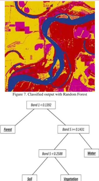
The second scene is of the Mississippi bottomland at 34 19 33.7518 N latitude and 90 45 27.0024 W longitude and acquired on 23 September, 2014. The Mississippi scene is shown similarly in bands 5, 6, and 7 in Figure 5. Training and test data were acquired in the same manner as the Yellowstone scene. Classes of water, soil, forest, and agriculture were chosen and spectral signatures are shown in Figure 6. The scene was also classified using neural network, support vector machine, minimum distance, maximum likelihood and ID3 classifiers. The classified output from Random Forest is shown in Figure 7, and the ID3 tree is shown in Figure 8.

Figure 5. Mississippi Scene (Raw)

_______________________________________________________________________________________

Figure 7. Classified output with Random Forest

Figure 8. ID3 Tree for Mississippi Scene IV. CONCLUSIONS

In this research we developed simulation for Random Forest and analyzed two Landsat scenes acquired with Landsat-8 OLI. The scenes were analyzed using ERDAS Imagine and the R package by Liaw and Wiener [23]. It can be seen from Table 2 that the performance of Random Forest was better than all other classifiers in terms of overall accuracy and kappa coefficient. Table 3 shows that Random Forest was outperformed by the neural network and support vector machine. This could be due to impure training sets. Random Forest works well given large homogeneous training data and is relatively robust to outliers.

As the Yellowstone scene contained dips in elevation, the reflectance of the bands altered as valleys became shadows. We found that training the forest with the shadowed areas increases the classification error of the forest. Generally, with a large number of training samples, Random Forest performs better [22]. The Mississippi scene was trained with homogeneous samples. This led to high accuracy of Random Forest that outperformed all other classifiers.

Table 2. Classification Results (Yellowstone Scene)

Classifier Overall Accuracy Kappa Coefficient Random Forest 96% 0.9448 ID3 Tree 92.5% 0.8953 Neural Networks 98.5% 0.9792 Support Vector Machine 99% 0.9861 Minimum Distance Classifier 100% 1.0 Maximum Likelihood Classifier 92.5% 0.8954

References

[1] D. Lu and G. Weng, “A survey of image classification methods

and techniques for improving classification performance”, Int. Journal of Remote Sensing, vol. 28, no. 8, 2004, pp 823-870.

[2] D. A. Landgrebe, “Signal Theory Methods in Multispectral

Remote Sensing”, John Wiley, Hoboken, NJ, 2003.

[3] K. S. Chen, Y. C. Tzeno, C. F. Chen, and W. I. Kao. Land cover classification of multispectral imagery using dynamic learning neural network. Photogrammetric Engineering and Remote Sensing, vol. 81. 1995, pp. 403-408.

[4] G. M. Foody. Supervised classification by MLP and RBN neural networks with and without an exhaustive defined set of classes. International Journal of Remote Sensing, vol. 5, 2004, pp 3091-3104.

[5] W. Y. Huang and R. P. Lippmann, “Neural Net and Traditional

Classifiers,” in Neural Information Processing Systems, 1988, pp. 387–396.

[6] S. J. Eberlein, G. Yates, and E. Majani, “Hierarchical multisensor analysis for robotic exploration,” in SPIE 1388, Mobile Robots vol.. 578, 1991, pp. 578–586.

[7] A. Cleeremans, D. Servan-Schreiber, and J. L. McClelland, “Finite State Automata and Simple Recurrent Networks,” Neural Computation, vol. 1, no. 3, 1989, pp. 372–381.

[8] S. E. Decatur, “Application of neural networks to terrain

classification,” in International Joint Conference on Neural Networks, 1989, vol. 1, pp. 283–288.

[9] A. D. Kulkarni and K. Lulla, “Fuzzy Neural Network Models

for Supervised Classification: Multispectral Image Analysis,” Geocarto International, vol. 14, no. 4, 1999, pp. 42–51.

[10] R. H. Laprade, “Split-and-merge segmentation of aerial

photographs,” Computer Vision, Graphics, and Image Processing, vol. 44, no. 1, 1988, pp. 77–86.

[11] R. J. Hathaway and J. C. Bezdek, “Recent convergence results

for the fuzzy c-means clustering algorithms,” Journal of Classification, vol. 5, no. 2, 1988, pp. 237–247.

[12] S. K. Pal, R. K. De, and J. Basak, “Unsupervised feature

evaluation: a neuro-fuzzy approach.,” IEEE transactions on neural networks / a publication of the IEEE Neural Networks Council, vol. 11, no. 2, 2000, pp. 366–76..

[13] A. Kulkarni and S. McCaslin, “Knowledge Discovery From

Multispectral Satellite Images,” IEEE Geoscience and Remote Sensing Letters, vol. 1, no. 4, 2004, pp. 246–250.

[14] G. Mountrakis, J. Im, C. Ogole, “Support vector machines in

remote sensing: A Review: Int. Journal of Photogrammetry and Remote Sensing, vol. 60, 2011, pp 247-259.

[15] P. Mantero, G. Moser, S. B. Serpico, “ Partially supervised classification of remote sensing images through – SVM-based probability density estimation, IEEE Transaction on Geoscience and Remote Sensing, vol. 43, no. 3, 2005, pp 559-570.

[16] P. Mitra, B. Uma Shankar, and S. K. Pal, “Segmentation of

multispectral remote sensing images using active support vector machines,” Pattern Recognition Letters, vol. 25, no. 9, 2004, pp. 1067–1074.

[17] R. M. Hansen, R. Dubayah, and R. DeFries, “Classification

trees: an alternative to traditional land cover classifiers”, International Journal of Remote Sensing, vol. 17, 1990, pp 1075-1081.

[18] M. K. Ghose, R. Pradhan, and S. Ghose, “Decision tree

classification of remotely sensed satellite data using spectral separability matrix,” International Journal of Advanced

_______________________________________________________________________________________

Computer Science and Applications, vol. 1, no. 5, 2010, pp. 93–101.

[19] L. Breiman, “Random Forests,” Machine Learning, vol. 45, no.

1, 2001, pp. 5–32.

[20] P. O. Gislason, J. A. Benediktsson, and J. R. Sveinsson. “Random forest for land cover classification”, Pattern Recognition Letters, vol. 27, 2006, pp 294-300.

[21] J. Han, M. Kamber, and J. Pei, Data Mining: concepts and techniques, 3rd ed. Waltham, MA: Morgan Kaufmann, 2012.

[22] L. Breiman, J. H. Friedman, R. A. Olshen, and C. J. Stone, Classification and Regression Trees. Belmont, CA: Wadsworth International Group, 1984.

[23] R. O. Duda, P. E. Hart, and D. G. Stork, Pattern Classification, 2nd ed. New York, NY: John Wiley & Sons, Inc., 2001, pp. 394–434.

[24] J. R. Quinlan, “Induction of Decision Trees,” Machine

Learning, vol. 1, no. 1, 1986, pp. 81–106.

[25] L. Breiman, “Bagging predictors,” Machine Learning, vol. 24,

no. 2, 1996, pp. 123–140.

[26] M. Pal and P. M. Mather, “Decision Tree Based Classification

of Remotely Sensed Data,” 22nd Asian Conference on Remote Sensing, 2001.

[27] L. Breiman and A. Cutler, “Random Forests,” 2007. [Online].

Available:

https://www.stat.berkeley.edu/~breiman/RandomForests/. [Accessed: 08-Aug-2014].

[28] A. Liaw and M. Wiener, “Classification and Regression by

randomForest,” R News, vol. 2, no. 3, 2002, pp. 18–22.

[29] B. Lowe and A. D. Kulkarni. “Multispectral image analysis

using Random Forest”, International Journal on Soft Computing (IJSC), vol. 6, no.1, 2015, pp 1-14.

[30] R. G. Congalton, “A review of assessing the accuracy of

classifications of remotely sensed data,” Remote Sensing of Environment, vol. 37, no. 1, 1991, pp. 35–46.

[31] “Wildland Fire Activity in the Park,” 2014. [Online].

Available:

http://www.nps.gov/yell/parkmgmt/firemanagement.htm. [Accessed: 10-Nov-2014].