CLASSES OF BYZANTINE FAULT-TOLERANT
ALGORITHMS FOR DEPENDABLE
DISTRIBUTED SYSTEMS
ISBN 90-365-1081-3
Copyright
1998 by A. Postma
All rights reserved. No part of this publication may be reproduced, stored
in a retrieval system, or transmitted, in any form or by any means,
elec-tronic, mechanical, photocopying, recording, or otherwise, without prior
written permission of the author.
CLASSES OF BYZANTINE FAULT-TOLERANT
ALGORITHMS FOR DEPENDABLE
DISTRIBUTED SYSTEMS
PROEFSCHRIFT
ter verkrijging van
de graad van doctor aan de Universiteit Twente,
op gezag van de rector magnificus,
prof. dr. F.A. van Vught,
volgens besluit van het College voor Promoties
in het openbaar te verdedigen
op vrijdag 20 februari 1998 te 15.00 uur.
door
André Postma
geboren op 19 augustus 1968
te Aalst-Waalre
Dit proefschrift is goedgekeurd door de promotor:
Prof. Dr. Ir. Th. Krol
TABLE OF CONTENTS
Page
1.
Introduction
1
Abstract 1
1.1.
Dependable computer systems
1
1.1.1. Dependability attributes 2
1.1.2. The impairments to dependability 3
1.1.2.1. Faults, errors, and failures 3
1.1.2.2. Fault and failure classification 3
1.1.3. Dependability measures 5
1.1.4. The means of dependability 7
1.1.5. Overview 11
1.2.
Fault detection techniques
11
1.2.1. Duplication 11
1.2.2. Error-detecting codes 12
1.2.3. Checksums 12
1.2.4. Self-checking and fail-safe logic 12
1.2.5. Watch-dog timers and bus timeouts 13
1.2.6. Consistency and capability checks 13
1.2.7. Processor monitoring 14
1.2.8. Program monitoring 14
1.3.
Fault-tolerance techniques
14
1.3.1. Masking redundancy techniques 15
1.3.1.1. N-modular redundancy 15
1.3.1.2. Error-correcting codes 16
1.3.1.3. Masking logic 17
1.3.1.4. N-version programming 17
1.3.2. Dynamic redundancy techniques 17
1.3.2.1. Reconfigurable duplication 17
1.3.2.2. Reconfigurable N-modular redundancy 18
1.3.2.3. Backup sparing 18
1.3.2.4. Graceful degradation 18
1.3.2.5. Forward and backward error recovery 19
1.4.
Evaluation of techniques to improve the reliability and
1.5.
Overview of this thesis
21
1.6.
References
22
2.
A System Model
25
Abstract 252.1.
Introduction
25
2.2.
System model
26
2.3.
Description of the Dependable Distributed Data Storage
System
28
2.4.
Resilience to Byzantine faults
32
2.4.1. A restricted Byzantine fault model for lock-step synchronous systems 33 2.4.2. A restricted Byzantine fault model for a distributed system in which
protection against malicious intruders is required 35
2.5.
Conclusion
37
2.6.
References
37
3.
Authenticated Byzantine Agreement Protocols
39
Abstract 39
3.1.
Introduction
40
3.1.1. Consensus protocols 41
3.1.2. Interactive consistency algorithms 43
3.1.3. Byzantine Agreement Protocols 44
3.1.4. Classification of Byzantine Agreement Protocols 47 3.1.4.1. Classification of BAPs according to the synchrony of the
system 47
3.1.4.2. Classification of deterministic BAPs according to message
authentication 49
3.1.5. Reduction of the communication overhead of an authenticated BAP 51 3.1.6. Guaranteeing Byzantine Agreement under less strict synchronicity
assumptions 53
assumptions 58
3.2.
Authenticated Byzantine Agreement Protocols based on
encoding messages into symbols of an erasure-correcting code
59
3.2.1. The Authenticated Dispersed Joined Communication algorithms 60
3.2.1.1. Definitions 61
3.2.1.2. Construction of ADJC-algorithms 64
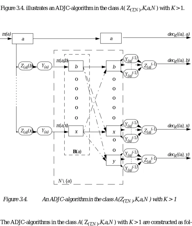
3.2.1.3. The existence of ADJC-algorithms in the classes
A(Z(T,N),K,a,N) 67
3.2.1.4. Behavioural properties of the ADJC-algorithms in the presence of at most Z(T,N) maliciously behaving processors 71 3.2.2. A class of Byzantine Agreement Protocols based on the
ADJC-algorithms 74
3.2.3. The construction of authenticated Byzantine Agreement Protocols
based on erasure-correcting codes 74
3.2.3.1. The Minimum Direction protocols 75
3.2.3.2. The Maximum Coding protocols 75
3.2.4. A comparison with existing BAPs 76
3.2.4.1. The criteria 76
3.2.4.2. The Lamport-protocol 76
3.2.4.3. The Dolev-protocol 76
3.2.4.4. The Minimum Direction protocol 77
3.2.4.5. The Maximum Coding protocol 78
3.2.4.6. Results 78
3.2.5. Conclusion 81
3.3.
Authenticated self-synchronizing Byzantine Agreement
protocols
81
3.3.1. Difference between authenticated self-synchronizing Byzantine Agreement Protocols and regular authenticated Byzantine Agreement
Protocols 81
3.3.1.1. Achieving protocol synchronization between correct
processors in a BAP 83
3.3.1.2. Path information 86
3.3.2. Informal description of an authenticated self-synchronizing BAP 88 3.3.2.1. Execution of an authenticated self-synchronizing BAP in
a system of correctly functioning processors only 88 3.3.2.2. Execution of an authenticated self-synchronizing BAP in
the presence of up to T maliciously behaving processors 90
3.3.3. The unforgeability properties 93
3.3.3.1. Valid messages 95
3.3.3.2. Generating a message 101
3.3.3.3. Relaying a message 101
3.3.3.4. Assumptions with regard to the authentication of messages 102 3.3.3.5. Satisfaction of the unforgeability properties 104 3.3.3.6. Final remarks on message authentication 109
3.3.4. Possible fault behaviour of faulty processors 110 3.3.5. Definitions with regard to the timeliness of valid messages 112 3.3.6. A description of an authenticated self-synchronizing BAP 113 3.3.7. A description of an optimized authenticated self-synchronizing BAP 116 3.3.8. Assumptions for authenticated self-synchronizing BAPs 119 3.3.9. Proofs for authenticated self-synchronizing BAPs 121 3.3.10. Proofs for optimized authenticated self-synchronizing BAPs 134 3.3.11. A comparison of authenticated self-synchronizing BAPs and
optimized authenticated self-synchronizing BAPs 143
3.3.12. Conclusion 145
3.4.
Authenticated self-synchronizing interactive consistency
algorithms
146
3.4.1. A description of an authenticated self-synchronizing ICA 146 3.4.2. A description of an optimized authenticated self-synchronizing ICA 157 3.4.3. A comparison of authenticated self-synchronizing ICAs and
optimized authenticated self-synchronizing ICAs 166
3.5.
References
168
4.
Distributed Cryptographic Function Application
Protocols
171
Abstract 171
4.1.
Introduction
172
4.1.1. Fault-tolerant data storage 172
4.1.2. Secure data storage 175
4.1.2.1. An introduction to cryptography 175
4.1.2.2. Protection of data against unauthorized reading by others 179 4.1.2.3. Protection of data against undetected mutilation by others 179 4.1.2.4. Protection of data against unauthorized reading and
undetected mutilation by others 183
4.1.3. Fault-tolerant and secure data storage 184
4.1.3.1. Different solutions for fault-tolerant and secure data storage 184 4.1.3.2. Evaluation of the proposed alternatives for fault-tolerant
and secure data storage 186
4.1.3.3. Recovery of lost or corrupted data fragments requires knowledge of the secret cryptographic function of the
cryptosystem applied for signing and verification 189 4.1.3.4. Distributed cryptographic function application protocols 190 4.1.3.5. A possible implementation of the recovery service 193 4.1.3.6. A possible implementation of the
4.1.4. Related work 200
4.1.4.1. Multisignature schemes 201
4.1.4.2. Secret sharing schemes 203
4.1.4.3. Threshold cryptography 205
4.1.5. Overview 207
4.2.
Distributed cryptographic function application protocols
based on a fault-tolerant multisignature scheme
208
4.2.1. Component cryptographic functions 209
4.2.2. Component cryptographic keys 210
4.2.3. Possible component cryptographic key distributions for DCFAPs based
on a fault-tolerant multisignature scheme 211
4.2.3.1. A component cryptographic key distribution which is
optimal with regard to the required number of processors 211 4.2.3.2. A component cryptographic key distribution which requires
a smaller number of different component cryptographic keys and a smaller number of copies of component cryptographic
keys 213
4.2.3.3. Comparison of the proposed component cryptographic key
distributions 215
4.2.4. Distributed cryptographic function application 218
4.2.4.1. Assumptions 220
4.2.4.2. Description of a PCFAP based on a fault-tolerant
multisignature scheme 223
4.2.4.3. Description of a DCFAP based on a fault-tolerant
multisignature scheme 232
4.2.5. Efficiency considerations on PCFAPs based on a fault-tolerant
multisignature scheme 237
4.2.5.1. Partial cryptographic function application protocols with
completed paths of minimal length only 238
4.2.5.2. A method to reduce the number of completed paths in
partial cryptographic function application protocols 240
4.2.6. Summary 243
4.3.
Distributed cryptographic function application protocols
based on function sharing
244
4.4.
Comparison of DCFAPs based on a fault-tolerant multisignature
scheme with DCFAPs based on function sharing
251
4.5.
Conclusion
252
5.
A Byzantine Fault-Tolerant Distributed
Diagnosis Algorithm
257
Abstract 257
5.1.
Introduction
257
5.2.
A distributed diagnosis algorithm with imperfect tests
258
5.2.1. Assumptions 260
5.2.2. Reduction rules 260
5.2.3. Classification of the remaining processors after having applied the
reduction rules 262
5.2.4. Examples of the use of the reduction rules 263
5.3.
Determining the maximum number of correct processors
removed from the service by the diagnosis algorithm
264
5.4.
Determining the maximum number of processors in the
service that are accused of being faulty
268
5.5.
Determining the minimally required number of processors
in the service
269
5.6.
Conclusion
269
5.7.
References
269
Appendix 5.1. Proof of correctness of the reduction rules
270
Appendix 5.2. Proof of consistency of the reduction rules
274
6.
Conclusion
279
Abstract 279
6.1.
Evaluation of results
279
6.1.1. Authenticated Byzantine Agreement Protocols 280 6.1.2. Distributed cryptographic function application protocols 282 6.1.3. A Byzantine fault-tolerant distributed diagnosis algorithm 283
6.2.
Suggestions for further research
284
6.3.
References
285
Abstract
287
Samenvatting
293
List of Publications
299
Acknowledgements
300
Biography
301
C H A P T E R 1
Introduction
“Perhaps all one can really hope for, all I am entitled to, is no more than this: to write it down. To report what I know. So that it will not be possible for any man ever to say again: I knew nothing about it.”
André Brink, A dry white season
Abstract
The omnipresence of computer systems in today’s society creates a need for highly dependable computer systems. In this chapter, dependability and its attributes (availa-bility, relia(availa-bility, safety, confidentiality, integrity, and maintainability) are defined. Depending on the applications considered, different emphasis may be placed on the different attributes of dependability. In dependable computing, the reliability and availability of computer systems have since long played an important role. Basically, there exist four techniques to improve the reliability and availability of a computer sys-tem: fault avoidance, fault detection, masking redundancy, and dynamic redundancy. It will be argued that repairable systems should be based on masking redundancy, in case the reliability and availability improvement should be a factor 100 or more, if compared to an equivalent system (i.e., satisfying the same specifications) in which no measures are taken in order to improve the reliability or availability of the system. In this thesis, we will present several new fault-tolerant protocols that may be imple-mented in a distributed fault-tolerant system based on masking redundancy.
1.1. Dependable computer systems
During the past few decades, the use of computer systems has taken a high flight. The ever increasing use of computers in almost every aspect of modern life makes us more and more dependent on the correct functioning of computers.
Practical experience has shown us that failures of computer systems which perform vital functions may have serious economic consequences, or may even endanger human lives. To illustrate this, Laprie (in [Lapr94]) mentions a few recent examples of nation-wide computer-caused or computer-related failures: the 15 January 1990 tele-phone service breakdown in the USA, the 26-27 June 1993 credit card authorization denial in France, and the 26-27 November 1992 London Ambulance Service failure. Whereas failure of the computer system in the first two examples had primarily eco-nomic consequences, the third example shows that failures may even lead to loss of human lives. From these examples, it will be clear that in several critical applications, it is very important to minimize the probability of the occurrence of a system failure.
2 1. INTRODUCTION
A system failure occurs when the actual system behaviour is inconsistent with the specified system behaviour. Roughly spoken, at a system failure, the system reacts on certain input in a way, different from what the user expects. Failures are caused by faults1 in the components or the software of the system. Faults may occur due to numerous causes, e.g., physical defects of electrical components, execution of incor-rectly designed programs, or operator mistakes.
In general, avoiding a system failure is of utmost importance in either of the following cases [Aviz76]:
❏ the real-time delays caused by manual repair after system failure are unacceptable (e.g., in systems with hard real-time constraints, like process control applications, guidance systems, air traffic control systems, and fly-by-wire)
❏ it is impossible to manually repair the system (e.g., in systems that have to be unmanned, like systems used for space exploration)
❏ the costs of lost time and maintenance are excessively high (e.g., in banking applications, life-critical support systems, and defense systems)
Basically, it can be concluded that there exists an increasing need for so-called depend-able computer systems. The concept of dependability was originally introduced by Laprie in [Lapr85] in an attempt to create a consistent terminology in the field of relia-ble computing. Dependability is defined as that property of a computer system such that reliance can be justifiably placed on it. Clearly, this is still a rather vague defini-tion. In general, it depends heavily on the requirements made for the application, whether or not reliance can justifiably be placed on a system.
The notion of dependability can more precisely be specified by distinguishing a number of aspects of dependability of a computer system, the relevance of which may differ for every application that is considered. In [Lapr85,Lapr92, Lapr95], Laprie has distinguished dependability attributes, impairments, measures, and means. The remainder of this section will be devoted to the aspects of dependability just men-tioned.
1.1.1. Dependability attributes
In [Lapr95], dependability is defined as that property of the computer system such that reliance can justifiably be placed on the service it delivers. The service delivered by a system is its behaviour as it is perceived by its user(s). A user is another system (phys-ical, human), which interacts with the former.
Dependability consists of the following so-called attributes (cited from [Lapr95]):
❏ availability (i.e., readiness for usage)
❏ reliability (i.e., continuity of service delivery)
❏ safety (i.e., non-occurrence of catastrophic consequences on the environment)
❏ confidentiality (i.e., non-occurrence of unauthorized disclosure of information)
❏ integrity (i.e., non-occurrence of improper alterations of information)
❏ maintainability (i.e., aptitude to undergo repairs and evolution)
Depending on the application(s) intended for the system, different emphasis may be
1. INTRODUCTION 3
put on the different attributes of dependability [Lapr95].
1.1.2. The impairments to dependability
Besides the attributes of dependability, Laprie also distinguishes between the so-called impairments to dependability: faults, errors, and failures. In Section 1.1.2.1., we give exact definitions of fault, error, and failure. These definitions are taken from [Lapr95]. In Section 1.1.2.2., several possible classifications of faults and failures are presented.
1.1.2.1. Faults, errors, and failures
A failure of the system occurs when the delivered service first deviates from that required by its specifications. An error is that part of the system state which is liable to lead to subsequent system failure. That means, if there is an error in the system state, then there exists a sequence of actions which can be executed by the system and which will lead to system failure, unless some corrective measures are employed [Jalo94, p.6]. The (adjudged or hypothesized) cause of an error is a fault. There are numerous reasons why a fault may occur, e.g., the occurrence of a physical defect, incorrect design, operator mistakes, unstable hardware, or an unstable environment.
1.1.2.2. Fault and failure classification
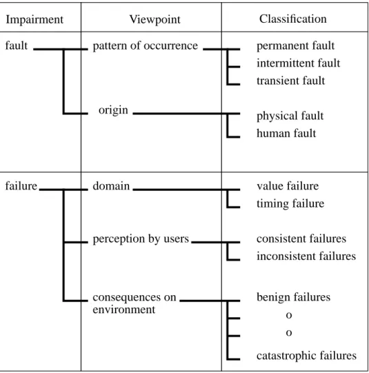
Both faults and failures can be characterized according to different viewpoints. The different viewpoints, as well as the different types of faults respectively failures that can be distinguished according to any of the viewpoints, are given in Figure 1.1. The characterization of failures in Figure 1.1. is taken from [Lapr95]. The classification of faults is taken from [SiSw92, pp.22-23].
According to the viewpoint of pattern of occurrence, in Figure 1.1., classes of perma-nent, intermittent, and transient faults are distinguished. In [SiSw92, p.22], these types of faults are defined as follows. A permanent fault is a fault that is continuous and sta-ble. In hardware, permanent faults reflect an irreversible physical change. An intermit-tent fault is a fault that is only occasionally present due to unstable hardware or varying hardware or software states. A transient fault is a fault resulting from tempo-rary environmental conditions. The major difference between intermittent faults and transient faults, is that intermittent faults may be detectable and repairable by replace-ment or redesign, whereas transient faults are incapable of repair because the hardware is physically undamaged [SiSw92, p.22].
From the viewpoint of origin of the faults, physical faults and human faults are distin-guished. In [SiSw92, p.22], these classes of faults are defined as follows. A physical fault is a fault which stems from physical phenomena internal to the system, such as threshold changes, shorts, opens, etc., or external changes, such as environmental, electromagnetic, vibration, etc. Human faults may be either design faults, which are committed during system design, modification, or establishment of operating proce-dures, or they may be interaction faults, which are violations of operating or mainte-nance procedures.
A different way to classify faults and failures, described in, e.g., [Cris91, BaMD93, Alst96], is to mathematically describe the fault behaviour of components, i.e., the behaviour that a component may exhibit once it is faulty. Every fault class is deter-mined by the fault behaviour that is allowed for faults in that fault class. The advantage
4 1. INTRODUCTION
of this approach is that the behaviour of the system can be mathematically described, while taking into account that several components may be faulty. Barborak et al. (in [BaMD93]) order the fault classes in a hierarchical way. The classes, from strongest to weakest, are fail-stop faults, crash faults, omission faults, timing faults, incorrect com-putation faults, authenticated Byzantine faults, and Byzantine faults. Each of the classes will be defined below. An interesting property is that a stronger class is a subset of a weaker class [BaMD93, p.182]. The stronger the fault model that is assumed, the easier becomes the solution that takes into account this fault behaviour [LaSP82, p.401]. The ordered fault classification depicted in Figure 1.2. is taken from [BaMD93, p.183].
The definitions of the various fault classes given below are taken from2 [BaMD93, pp.182-183].
The class of fail-stop faults contains any fault that occurs when a processor ceases operation and alerts other processors of this fault (originally defined in [ScSc83]). The
2. Except the definition for the class of omission faults, which was taken from [Cris91].
Figure 1.1. Fault and failure classification according to different view-points
Impairment Viewpoint Classification
fault pattern of occurrence permanent fault intermittent fault transient fault origin
physical fault human fault
failure domain value failure
timing failure perception by users consistent failures
inconsistent failures consequences on environment benign failures catastrophic failures o o
1. INTRODUCTION 5
class of crash faults consists of any fault that occurs when a processor loses its internal state or halts. The class of omission faults is defined as the class of faults that occur when a processor omits to respond to an input [Cris91]. The class of timing faults encompasses any fault that occurs when a processor fails to complete its task within the specified time frame, i.e. it completes its task either before or after its specified time frame or never [CASD95]. The class of incorrect computation faults contains any fault that occurs when a processor fails to produce the correct result in response to the correct inputs [LaMJ91] 3. The class of authenticated Byzantine faults contains any arbitrary or malicious fault, with that exception that faulty processors are not capa-ble of imperceptibly altering a message signed by a correct processor. Faulty proces-sors may collude with other faulty procesproces-sors [LaSP82]. The class of Byzantine faults contains every arbitrary or malicious fault that is possible in the system model [LaSP82]. This fault class can be considered the universal fault set [BaMD93, p.183].
1.1.3. Dependability measures
In literature, the dependability of the system can be quantified by many different func-tions, the so-called dependability measures. A number of these dependability meas-ures will be mentioned below. Which dependability measure is most adequate to
3. The incorrect computation fault class is a superset of the crash, omission and timing fault classes and a subset of the class of Byzantine failures. The first characteristic is true because a miscalculation may take place in time and space. Since the fault is consistent to all outside observers, though, the class of incorrect computation faults is a subset of the class of Byzan-tine failures [LaMJ91, BaMD93].
Figure 1.2. An ordered fault classification fail-stop crash omission timing incorrect computation authenticated Byzantine Byzantine
6 1. INTRODUCTION
express the required dependability of the system, depends on the specific application that is considered.
Below, dependability measures will be presented to express the reliability and the availability of the system. Quantifications of the other dependability attributes (i.e., safety, confidentiality, integrity, and maintainability) are hardly found in literature. We will not try to quantify them here either. Whether or not these dependability attributes play an important role, is highly application-dependent.
Usually, the reliability of a system is expressed as a function R(t), which is (infor-mally) defined as the probability that the system has not suffered from a system failure until time t (t > 0), provided that the system initially (i.e., at time 0) works correctly [Jalo94, p.34]. The mean time to failure (MTTF), or expected life [Jalo94. p.34] of a system can be expressed in terms of R(t) as follows:
The above dependability measures may be adequate, e.g., in non-repairable systems, i.e., systems in which faulty components are not repaired, like unmanned space mis-sions.
However, for telecommunication services, it is important that the fraction of time that the system is down is kept as small as possible, and thus, failed components should be repaired as quickly as possible. In this case, it is more adequate to express the required dependability of the system in terms of the availability of the system, i.e., the fraction of the time that the system is not out of operation [Krol91, p.17].
In [Jalo94, p.37], the instantaneous availability, A(t), of a component is defined as the probability that the component is functioning correctly at time t. In availability analy-sis, we are interested in probability at a certain instance of time. In the absence of repair or replacement, availability is simply equal to reliability. However, often, replacement is taken into account, and in this case, in availability analysis, we are interested in availability after a sufficiently long time. The limiting availability (com-monly referred to as the availability) of a system is the limiting value of A(t) as t approaches infinity.
Krol (in [Krol91, p.17]) mentions several other dependability measures: the mean time between failures (or MTBF), the mean time between down (MTBD), and the mean time to repair (MTTR). In [Krol91], these dependability measures are defined as fol-lows.
The mean time between failures is defined as the expected length of the time interval between the moment the system is started up or a previous failure has been repaired and the moment at which a (subsequent) failure appears. The mean time between down is defined as the expected length of the time interval between the moment the system is started up (possibly after a repair) and the moment at which the system loses its functionality due to the occurrence of a fault. The mean time to repair is defined as the expected length of the time interval between system down and system up.
MTTF R t( )dt 0
∞
∫
1. INTRODUCTION 7
The (limiting) availability can be expressed as a function of MTTF and MTTR as fol-lows [Triv82]:
Jalote (in [Jalo94, p.38]) notices that the above expression is not dependent on the nature of the probability distributions of lifetimes and repair times. In other words, this expression holds for probability distributions other than the exponential distribution as well.
The effect of the measures to improve the reliability of a system can be expressed in terms of a so-called reliability improvement factor [Krol91, p.18]. Let S be a system in which measures are taken to improve the reliability of the system, and let the resulting system be S’. Then, the reliability improvement factor is defined as the quotient of the MTBD of system S’ and the MTBD of system S.
1.1.4. The means of dependability
This section contains a description of the means of dependability, i.e., the techniques that can be used in order to improve the dependability of a computer system, or more specifically, to improve several important attributes of the dependability of a computer system. The reliability and availability of computer systems have since long played an important role in the field of reliable computing, and many techniques are known to improve the reliability and availability of a computer system. Therefore, in this sec-tion, we will focus on techniques that can be used to improve these two attributes of dependability.
Basically, there exist four different techniques to improve the reliability and availabil-ity of a system: fault avoidance, fault detection, masking redundancy, and dynamic redundancy. Each of these techniques will be discussed below.
A direct approach to improve the reliability and availability of the system is to try to prevent faults from occurring or getting introduced in the system. This approach is called fault avoidance or fault prevention [Lapr85, Lapr92, Lapr95].
In the approach of fault avoidance, a highly reliable and available system is obtained by eliminating as many faults as possible before the system is put into regular use. This is achieved by extensively testing the system software as well as the behaviour of all components needed for the system, and, while building the system, by applying only those components and software which exhibit correct behaviour during the tests. Such a system is a non-redundant system, i.e., it does not contain redundancy (i.e., it does not contain components or perform checks or other computations that are superfluous as long as all components in the system function correctly). A system failure may occur as soon as a fault occurs in one or more components of the system. Although enormous improvements have been made with regard to the technical quality of com-puter system components, it is obvious that failures of comcom-puter systems can never be ruled out completely [Powe91, p.9]. E.g., it is known that electrical components are subject to environmental conditions (causing them to wear out) and hence, such com-ponents will sooner or later fail to satisfy their specification. Upon system failure, the
A t( ) t→∞ lim MTTF MTTF+MTTR ---=
8 1. INTRODUCTION
system needs to be repaired. In the meantime, the system is down (i.e., not in opera-tion). For several critical applications, like the ones described above, it is highly important that the probability that a system failure occurs is being made as small as possible.
By means of applying fault prevention techniques, the reliability of the system can be improved by a factor 10 without exceptionally high costs [Krol91, p.18].
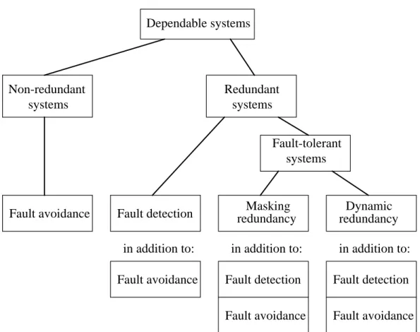
In order to improve the reliability and availability of the system beyond that what can be reached by applying fault prevention techniques, one should not only try to prevent faults from occurring or being introduced in the system, but, in addition, the system should be designed in such a way that the occurrence of faults during operation is taken into account. Thus, besides fault prevention techniques, techniques of fault detection, masking redundancy (also called static redundancy), and/or dynamic redundancy should be applied in the design of a dependable system. Application of either of these techniques requires the system to be a so-called redundant system, i.e., a system in which redundancy is applied. Whereas systems based merely on fault detection and/or fault avoidance can only guarantee that the specified service is pro-vided until a fault occurs, systems based on masking redundancy and/or dynamic redundancy may even continue to provide the correct service despite the occurrence of one or more faults in the system. The latter systems are therefore often called fault-tol-erant systems4. A schematic overview of dependable systems (analogous to [SiSw92, p.83]) is given in Figure 1.3.
In systems based on fault detection, redundancy is applied in order to detect faults. Usually, upon detection of faults, the system reports occurrence of a fault, after which the system is brought down, diagnosed, and manually reconfigured to allow a restart [SiSw92, p.82]. Some hardware techniques used for fault detection are duplication, error-detecting codes, checksums, self-checking and fail-safe logic, watch-dog timers and bus timeouts, consistency and capability checks, and processor monitoring. A soft-ware technique used for fault detection is program monitoring. Each of these tech-niques will briefly be discussed in Section 1.2. For more details on these techtech-niques, see, e.g. [SiSw92, pp. 96-138].
In fault-tolerant systems, redundancy is applied in order to tolerate faults. I.e., the sys-tem contains components (hardware redundancy), or performs checks or other com-putations (software redundancy) which are not required (i.e., redundant) as long as all components of the system function correctly. The redundancy aims to enable the sys-tem to continue to deliver the specified syssys-tem service despite the presence of faulty components in the system. This is in contrast with systems based on fault avoidance or fault detection techniques, in which a failure of a system component may lead to a sys-tem failure.
In most fault-tolerant systems, redundancy is applied in the form of both software
4. Systems that are based on fault detection techniques are usually not regarded as fault-tolerant systems [SiSw92, p.83], since these systems are not capable of tolerating any type of fault. In particular, a system based on fault detection techniques cannot tolerate permanent faults, although permanent faults may be detected by such a system. Transient and intermittent faults (see Section 1.1.2.2.) may only be tolerated by using retry techniques.
1. INTRODUCTION 9
redundancy (or time redundancy) and hardware redundancy (or component redun-dancy). Systems not containing hardware redundancy can not be made resilient to per-manent component failures5. By applying hardware redundancy, a system can be made resilient to permanent component failures.
In systems based on masking redundancy, redundancy is applied in order to mask fail-ures of components of the system. The system may continue to provide the specified service as long as the number of component failures stays below a predefined maxi-mum. Several hardware techniques used in systems based on masking redundancy are, e.g., N-modular redundancy, error-correcting codes, and masking logic. A software technique is N-version programming. A short investigation of each of these techniques will follow in Section 1.3.1. For more details, see, e.g., [SiSw92, pp. 138-169, and pp. 206-213].
In systems based on dynamic redundancy, upon component failures, the system is dynamically reconfigured so as to on-line replace the failed components by correctly functioning spare components. Several hardware techniques used in systems based on dynamic redundancy are, e.g., reconfigurable duplication, reconfigurable N-modular redundancy, backup sparing, and graceful degradation. Software techniques are, e.g.,
5. See Section 1.2.2. Dependable systems Non-redundant systems Redundant systems
Fault avoidance Fault detection redundancyMasking redundancyDynamic Fault-tolerant
systems
Figure 1.3. Schematic overview of dependable systems Fault avoidance Fault detection
Fault avoidance
Fault detection Fault avoidance in addition to: in addition to: in addition to:
10 1. INTRODUCTION
backward and forward error recovery. Section 1.3.2. provides a short introduction to each of these techniques. For more details, see, e.g., [SiSw92, pp. 169-201, and pp. 213-219].
In order to improve the reliability and availability of a system, often, a combination of techniques is used, i.e., the design of a dependable system involves application of tech-niques of fault-avoidance, fault-detection and fault-tolerance.
In a redundant system, treatment of faults that occur in the system may consist of a number of steps, discussed below. In these steps, the above-mentioned techniques of fault-detection and fault-tolerance may be used as indicated below.
According to [SiSw92, pp.80-82], fault treatment consists of the following steps: 1. Fault detection
In this initial step, it is detected that something unexpected has happened in the system. Many techniques to detect faults exist (see Section 1.2.). In general, an arbitrary period of time, called the fault latency, has passed between the occur-rence and the detection of a fault. It is even possible that some faults (e.g., tran-sient faults, see Section 1.1.2.2.) are never detected.
2. Fault diagnosis
In this step, diagnosis is performed in order to obtain information about the loca-tion and/or the nature of the detected fault. This step is necessary if the fault detection technique does not provide this information.
3. Reconfiguration
This step occurs in case the detected fault has led to a permanent component fail-ure. In a system based on dynamic redundancy, reconfiguration may be done on-line by reconfiguring the system such as to replace the failed component by a backup spare. Alternatively, the failed component may be switched off and the system capability degraded in a process called graceful degradation ([SiSw92, p.81]). In a system which is not based on dynamic redundancy, reconfiguration has to be done off-line. In a system based on masking redundancy, the system may be able to continue its specified service despite the presence of faults. If a critical task is performed, reconfiguration may be postponed until the critical task has finished.
4. Recovery
In this step, the effects of faults are eliminated, either by means of techniques of fault masking or retry. Fault masking techniques hide the effects of component failures by having redundancy provide for sufficient correct information. In retry techniques, in case the occurrence of a fault inhibits execution of a certain opera-tion, it is tried multiple times to execute this operation. For transient or intermit-tent faults (see Section 1.1.2.2.), this approach may be successful.
5. Restart
Once recovery has been finished, the system can be restarted. A hot restart (i.e., a resumption of all operations from the point of fault detection ([SiSw92, p.81]) is
1. INTRODUCTION 11
only possible if the fault did not cause permanent damage. Otherwise, a warm restart (i.e., some of the processes can be resumed without loss) or a cold restart (i.e., a re-initialization of the system) is required.
6. Repair
In this step, a failed component is replaced. In systems based on masking redun-dancy, the component can be replaced on-line (i.e., without interrupting system operation) if for a sufficiently long period of time, the component is not necessary for operation, e.g., if the component is temporarily idle. Otherwise, the compo-nent has to be replaced off-line. In systems based on dynamic redundancy, the component may be replaced on-line by a backup spare. In other systems, repair has to be done off-line.
7. Reintegration
In this step, the repaired component must be reintegrated into the system. For on-line repair, reintegration must take place without interrupting system operation. In non-redundant systems, only fault avoidance techniques can be applied, and human intervention is required in all steps of fault treatment given above. In redundant sys-tems, it is also possible to apply techniques of fault detection, masking redundancy and / or dynamic redundancy. In such a system, one or several of the fault treatment steps can be automated.
Since redundancy is applied in fault-tolerant systems, these systems are usually more expensive (in terms of hardware and/ or computation time) than systems which pro-vide the same functionality but which are not fault-tolerant. The more reliable and available we want to make the system, the more redundancy is required, and, inher-ently, the more expensive the system will be. In practice, the design of a fault-tolerant system is mainly determined by the allowed system costs and the performance, relia-bility and availarelia-bility that is required.
In this thesis, our focus will be on the design of algorithms that are used in fault-toler-ant systems, i.e., systems in which ultra-high dependability is required.
1.1.5. Overview
The rest of this chapter is structured as follows. Section 1.2. gives a more detailed dis-cussion of the fault avoidance techniques mentioned in Section 1.1.3. In Section 1.3., the previously mentioned fault-tolerance techniques are investigated. Section 1.4. eval-uates the techniques of Section 1.2. and 1.3. Finally, Section 1.5. provides an overview of the rest of this thesis.
1.2. Fault detection techniques
In this section, the fault detection techniques, as mentioned in Section 1.1.3., will sub-sequently be discussed.
1.2.1. Duplication
12 1. INTRODUCTION
component level or system-level). Duplication of a component (respectively, a system) consists of simply making a copy of the component (respectively, the system). Both copies have the same functionality. When a failure occurs in one of the copies, the two copies will no longer be the same, and a simple comparison will detect the fault. An advantage of using duplication is, that duplication successfully detects all single faults except that of the comparison element [SiSw92, p.97]. It is even possible to detect dou-ble faults, provided that the output of both copies is different. A disadvantage is that the method requires much redundancy. The cost of duplication is twice that of an equivalent simplex system, plus the cost of the comparison element [SiSw92, p.101]. The technique of duplication is applied in the commercially available systems from Tandem and Stratus.
1.2.2. Error-detecting codes
Error-detecting codes consist of systematically adding redundancy to information. Information is encoded into so-called code words, which are simply fixed-length sequences of bits. The code words contain redundant bits, which enables the set of code words of a certain length l (for some l > 1) to be only a subset of the set of all pos-sible words of length l, i.e., all pospos-sible sequences of bits of length l. Mutilations of code words can be detected, provided that the resulting word is not a code word. Many different coding techniques and error-detecting codes exist. An introduction to this subject can be found in [MaSl78, VaOo89].
1.2.3. Checksums
A cheap method of fault detection is checksumming. In fact, checksums are a form of error-detecting codes. The following description of a checksum is taken from [SiSw92, p.115]. The checksum for a block of s words is formed by adding together all of the words in the block modulo-n, where n is arbitrary. The block of s words and its check-sum together constitute a code word in a so-called linear separable code, i.e., a code in which the code words are formed by a concatenation of data bits and redundant bits, such that the two sequences of bits can be easily distinguished. The number of bits in the sum is usually limited. This quantity is compared with the checksum which was formed and stored at the moment the block was transmitted for the last time. Check-summing is cheap in terms of required redundancy. However, it has a number of disad-vantages. Main disadvantages are, that it takes a long time to detect faults (s additions and a comparison), the checksum must be updated on each write operation on the block, and the diagnostic resolution is low. Viz., in memories, the detected fault could be in the block of s words, the stored checksum, or the checking circuitry, whereas, in data transmission, the fault could be in the data source, the transmission medium, or the checking circuitry [SiSw92, p.115].
1.2.4. Self-checking and fail-safe logic
A disadvantage of the previously presented methods of duplication, error-detecting codes and checksums is that they all contain a single point of failure, i.e., a specific component in the system is not allowed to fail. The techniques of duplication and checksumming are vulnerable to a failure in the comparison element, whereas the tech-nique of error-detecting codes is vulnerable to a failure of the decoder. In order to avoid such single point of failures, self-checking logic has been introduced. See [SiSw92, p.124-130] for an overview.
1. INTRODUCTION 13
In [AnMe73, SiSw92], totally self-checking logic is defined as logic which is both self-testing and fault-secure. A self-testing circuit is defined as a circuit in which, for every fault from a prescribed set, the circuit produces a noncode output for at least one code input [Ande71, SiSw92]. A circuit is called fault-secure if, for every fault from a prescribed set, the circuit never produces an incorrect output for code inputs. A disad-vantage of application of totally self-checking logic is that much redundancy is required.
Alternatives in which fewer redundant elements are required, are partially self-check-ing logic, and fail-safe logic.
A circuit is partially self-checking if it is self-testing for a set N of normal inputs and a set Ft of faults, and it is fault-secure for a set I (a nonempty subset of N) and a set Fs of faults [SiSw91, p.126]. In partially self-checking logic, the required component redun-dancy is lower than that of duplication, be it, however, at the cost of an increased fault latency (i.e., undetected faults may exist for a while prior to detection).
A circuit is fail-safe, if, for every fault from a prescribed set, any input produces a ‘safe’ output, i.e., one of a preferred set of erroneous outputs [SiSw92, p.130]. Fail-safe techniques are thus not concerned with the detection of faults per se, and they can result in lower redundancy costs than self-checking techniques.
A disadvantage of applying the technique of self-checking or fail-safe logic is that it relies on only one of the gates in the circuit being defective. If all gates are integrated in an IC, this assumption applies to only a small percentage of possible faults [Krol91, p.23].
1.2.5. Watch-dog timers and bus timeouts
Watch-dog timers are used to keep track of the execution time needed by the system to perform a certain task. The timer is set before execution of a certain task by the system, indicating the maximum time that is allowed to perform this task. After having exe-cuted this task, the timer is reset. If the system works properly, it is always possible to timely reset the timer. However, if the system fails in some way, it may also fail to reset the timer, which may be detected as soon as the timer expires. Of course, the sys-tem may only partially fail, produce erroneous output and still be able to correctly reset its watch-dog timer. Since output data is not checked, not every failure is detected. However, the method is very effective, since many tasks fail in an infinite loop [Krol91, p.24], hence they fail to reset the watch-dog timer, and the failure can be detected.
In the method of bus timeouts, time limits are set for certain responses required by the bus protocol. E.g., when one device requires a response from another device, a failure to respond in time (which may indicate a possible failure) will be detected.
1.2.6. Consistency and capability checks
Consistency checks verify if inputs or computed results are reasonable. A simple example is a range check, i.e., a check whether an input or a computed result is within
14 1. INTRODUCTION
a valid range. Most computers use some form of consistency checking.
In capability checking, access to objects is limited to users with the proper authoriza-tion. Objects include memory segments and I/O devices; users might be processes or independent physical processors in a system [SiSw92, p.133]. One can think of read/ write protection of files as it is done in the UNIX operating system. Another method of capability checking is the use of passwords.
1.2.7. Processor monitoring
Besides duplication, processor monitoring may be an efficient way to detect logic con-trol failures and check standard microprocessors [SiSw92, p.134]. Processor monitor-ing techniques are classified accordmonitor-ing to the information monitored: control-flow checking techniques and assertion checking techniques.
Control-flow monitoring techniques detect sequence errors, i.e., errors which cause a processor to jump to an incorrect next instruction. Assertion checking techniques make use of properties of program data by periodically checking for program data. Assertion checking requires the user to identify invariant properties of program data and devise code that will check for these properties [SiSw92, p.136]. Examples of invariant properties include cases in which a value of a variable should always be within a particular range, the output value values of a function are related to the input values by the inverse of that function, and variable values in a set increase or decrease monotonically. Success of this method depends heavily upon the existence of invari-ants in an application.
1.2.8. Program monitoring
This software fault-detection technique consists of monitoring the execution of a piece of software step-by-step. For this purpose, so-called debuggers can be applied.
1.3. Fault-tolerance techniques
Two different fault-tolerance techniques can be distinguished: masking redundancy techniques and dynamic redundancy techniques. These techniques will be the subject of Section 1.3.1. and 1.3.2., respectively.
In systems based on masking redundancy, fault detection, fault localization and recov-ery are automatically performed by the system, and form a whole. In systems based on masking redundancy, failures are tolerated and do not cause system operation to be interrupted. Masking redundancy is used, e.g., in computers with error-correcting code memories or with majority-voted redundancy in a fixed configuration (i.e., the logical connections between circuit elements remain constant) [SiSw92, p.83].
In systems based on dynamic redundancy, it is possible to automatically perform fault detection, fault localization, reconfiguration, recovery and restarting. Dynamic redun-dancy covers those systems whose configuration can be dynamically changed in response to a fault, or in which masking redundancy, supplemented by on-line fault detection, allows on-line repair. Examples include multiprocessor systems that can degrade gracefully in response to processing element failures and triplicated systems
1. INTRODUCTION 15
that are designed for on-line repair [SiSw92, pp.83-84].
1.3.1. Masking redundancy techniques
In this section, the masking redundancy techniques mentioned in Section 1.1.3. are subsequently discussed.
1.3.1.1. N-modular redundancy
The concept of N-modular redundancy can be applied at all levels of system design. In N-modular redundancy, N (N > 2) copies of the original system (respectively circuit) are placed in parallel, and a majority vote is taken over the outputs of the copies. In this way, faulty behaviour of up toN / 2copies can be masked. Here, for any nonnega-tive integer value x,x is defined as the largest integer less than or equal to x. Usu-ally, N is chosen to be odd in order to avoid the uncertain state in which the output is a tie.
A well-known example of N-modular redundancy applied at system level is the so-called TMR-system (Triple Modular Redundant-system). In a TMR-system, the origi-nal system is triplicated (i.e., N = 3), and a majority vote is taken over the outputs. The majority vote is taken by a voter, which must also be triplicated in order to avoid a sin-gle point of failure. In Figure 1.4., a schematic representation of a TMR-system is given. It is easy to see that a failure in one of the three copies can be masked. The
masking is accomplished by means of a majority (two-out-of-three) vote on the system Figure 1.4. Schematic representation of a TMR-system
S S S S V V V single system TMR-system S = single system V = majority voter input input output output output output
16 1. INTRODUCTION
outputs.
Krol (in [Krol91, p.25]) mentions that, in general, the voters will be provided with additional hardware which records the fact that a fault has been masked and in which module it has occurred. In this way, fault localization can be automatically performed by the system.
Krol (in [Krol91, p.25-26]) also notices that the addition of redundancy must be done very carefully. Extra hardware increases the probability of defects, as a result of which the reliability may decrease instead of increase. To see this, consider the TMR-system sketched above. If a fault causes a failure of more than one of the three copies, the TMR-system will break down. It is therefore important to minimize the probability that such dependent faults occur. An approach to solve this problem is to subdivide the system into so-called fault isolation areas or fault containment units. Faults within a fault isolation area may be dependent, but faults in different fault isolation areas are independent.
However, for a TMR-system, it is very difficult to create a fault isolation area for each of the three subsystems, since, in practice, clock generators, supply voltages, and elec-tromagnetic pulses may be the cause of dependent faults, causing more than one sub-system to fail. In [Krol91, p.27], Krol shows that dependent faults may drastically decrease the reliability improvement factor.
1.3.1.2. Error-correcting codes
Error-correcting codes are the most commonly used means of masking redundancy [SiSw92, p.146]. Just like error-detecting codes, error-correcting codes are a means of systematically adding redundancy to information. Information is encoded into code words. The code words contain redundant bits in such a way that a limited number of faulty bits can always be corrected. How many faulty bits in a code word can be cor-rected depends on the so-called Hamming distance of the applied error-correcting code.
The Hamming distance of a code is the minimum number of bit positions in which any two words in the code differ [Jalo94, p.23]. Let d be the Hamming distance, D be the number of bit errors that can be detected, and C be the number of bit errors it can cor-rect, then the following relation is always true [Jalo94, p.23]:
d = C + D +1, with D≥C
This means that all codes with Hamming distance d > 2 can be applied for both error-correction and error-detection. Notice that, in the above relation, error-correction of bit errors implies that these errors are detected.
Let k be the number of symbols in a data word, and n be the number of symbols in a code word. From [MaSl78], we know that an error-correcting code capable of correct-ing up to T errors can be constructed if and only if n≥k + 2T. From [Krol91], we know that such a code always exists if the symbol size b satisfies b≥2log(n-1).
In regular binary codes like ASCII, the Hamming distance is 1 (i.e., the code contains code words that differ in only one bit position), hence, D = 0 and C = 0 (i.e., no
error-1. INTRODUCTION 17
detection and no error-correction is possible). Addition of a parity bit to each code word increases the Hamming distance to 2 (viz., if two original code words differ in one position, then the parity bits of these code words will also be different, creating a Hamming distance of 2). Codes with Hamming distance 2 can only detect single bit errors (i.e., D = 1).
A special kind of error-correcting codes are the so-called erasure-correcting codes. These codes are able to correct a number of erasures, i.e., erroneous bits of which the position in the code word is known. Let k be the number of symbols in a data word, and n be the number of symbols in a code word. From [VaOo89], we know that an erasure-correcting code capable of correcting up to T erasures can be constructed if and only if n ≥ k + T. From [Krol91], we know that such a code always exists if the symbol size b satisfies b≥2log(n-1). An example in which an erasure-correcting code can be used is a bus with a single parity bit in which a particular bit line is known to be failed.
Many different error-correcting codes have appeared in literature. For an overview, see, e.g., [MaSl78, VaOo89].
1.3.1.3. Masking logic
In contrast with the previous two techniques, masking logic includes fault masking at gate level. Masking logic usually requires massive use of redundant gates, hence, only few of the techniques are actually used [SiSw92, p.162]. All techniques employ redun-dant inputs to each gate. In this section, we will not further investigate masking logic, because of its sporadical use. For details about masking logic, see, e.g., [SiSw92, pp.161-169].
1.3.1.4. N-version programming
The concept of N-version programming (also called diverse programming or design diversity) consists of independently developing N versions of a program. The software versions are developed by independent design teams utilizing different design method-ologies, algorithms, compilers, run-time systems, and hardware components. An advantage is that the entire system may be more reliable than any single independently developed copy, although it is in general impossible to quantify the reliability improve-ment. The disadvantages are additional design costs, costs of concurrent execution, and potential sources of dependent faults. For more details, see, e.g., [SiSw92, pp.207-213].
1.3.2. Dynamic redundancy techniques
Dynamic redundancy techniques involve the reconfiguration of system components in response to failures [SiSw92, p.169]. The reconfiguration prevents failures from influ-encing system operation. In all dynamic redundancy techniques, reconfiguration and recovery are automatically performed by the system.
1.3.2.1. Reconfigurable duplication
The technique of duplication discussed in Section 1.2.1. can be used for fault detec-tion. However, a duplicated system is not fault tolerant, unless some adaptations are made to the system. The resulting system is called a reconfigurable duplicated system. In such a system, additional hardware is needed in order to detect which module is
18 1. INTRODUCTION
faulty in case the outputs of both systems are different. Upon localization of the faulty module, the system should be reconfigured, i.e., the faulty module is disconnected from the system, and the comparison element is disabled. The resulting simplex sys-tem still satisfies the syssys-tem specification. For more details, see [SiSw92, p.171-174].
1.3.2.2. Reconfigurable N-modular redundancy
The technique of N-modular redundancy discussed in Section 1.3.1.1. can be applied to tolerate a number of faulty modules. However, as discussed in Section 1.3.1.1., an N-modular redundant system is not capable of tolerating more than N / 2 faulty modules. By making some adaptations to the NMR-system, it is possible to have the system tolerate more than N / 2 faulty modules. The resulting system is called a reconfigurable N-modular redundant system. Basically, two different types of recon-figurable NMR-systems exist: systems based on hybrid redundancy, and systems based on adaptive voting. Both types of systems will be briefly discussed below. In systems based on hybrid redundancy, the technique of N-modular redundancy is combined with the technique of backup sparing (which will be discussed in the next section). The system is assumed to consist of (N+S) modules, N of which are active and S of which are passive (spare) modules. The system output is equal to the majority vote taken over the outputs of the N modules. If the outputs of the N modules are not all equal, but the output values of a majority of modules are still equal, then these mod-ules are assumed to be correct, and the other modmod-ules in the system are replaced by spare modules. As long as the number of faulty modules in the set of N active modules does not exceed T =N / 2 before reconfiguration can take place, the system can tol-erate the failure of up to P = (T + S) of its modules [SiSw92, p.175]. More details can be found in [SiSw92, pp.174-178].
Systems based on adaptive voting are N-modular redundant systems, in which the sys-tem output is determined by the weighted value of each of the output values of the modules. The weight factors are usually zero or one. For more details, see, e.g., [SiSw92, pp.178-182].
1.3.2.3. Backup sparing
A system based on backup sparing consists of (N+S) modules, N of which are active and S of which are passive modules. The system output is determined by taking a majority vote over the outputs of the N active modules. Upon failure of an active mod-ule, it is replaced by a spare module. The concept of backup sparing can also be com-bined with techniques other than N-modular redundancy. More details can be found in [SiSw92, pp.187-190].
1.3.2.4. Graceful degradation
The technique of graceful degradation differs from the previously discussed dynamic redundancy techniques in that in a gracefully degradable system, the redundant (spare) modules are also used for normal system operation, while in reconfigurable duplica-tion, reconfigurable N-modular redundancy, and backup sparing, the spare modules only perform useful work, if they have replaced a failed active module. As a conse-quence, upon failure of one or more modules of a gracefully degradable system, the performance and / or the functionality of the system will degrade, since the system function must in this case be carried out by fewer modules.
1. INTRODUCTION 19
1.3.2.5. Forward and backward error recovery
Forward and backward error recovery are the two major software dynamic redundancy techniques.
Forward error recovery (or roll-forward) attempts to continue operation with the cur-rent system state [SiSw92, p.213]. Forward error recovery is highly application-dependent and can only occasionally be applied, e.g., in a real-time control system in which a missed response to a sensor input can be tolerated.
Backward error recovery (or roll-back) uses previously saved correct state informa-tion as the starting point after a failure [SiSw92, p.213]. Basically, there exist four forms of backward error recovery: retry, checkpointing, journaling, and recovery blocks, each of which will be briefly discussed below.
Upon detection of an error, retry techniques aim at repairing the system, after which the operation affected by the error is retried [SiSw92, p.200]. If the error is transient, repair consists in pausing long enough for the transient error to disappear. If the error is permanent, then the system should be reconfigured. Reconfiguration can only remove the error, if it is possible to recover the system state before occurrence of the error. Checkpointing techniques consist of saving some subset of the system state at specific points (so-called checkpoints) during process execution. The information that must be stored is the subset of the system state (i.e., data, programs, machine state) that is nec-essary to the continued successful execution and completion of the process past the checkpoint [SiSw92, p.214]. Upon detection of an error, the system is repaired and the system and the process state is reset to the state stored in the latest checkpoint.
The journaling technique consists of making a copy of the initial state of the system, and storing all transactions that change the state of the system [SiSw92, p.216]. Upon detection of an error, the system can recover from this error by again starting from the initial state, and running through the transactions a second time. Journaling is consid-ered to be a simple but very inefficient backward error recovery technique.
Recovery blocks combine elements of checkpointing and backup alternatives, as such providing resilience to both software design faults and permanent and transient hard-ware faults [SiSw92, p.216]. The method minimizes the amount of state information backed up and releases the programmer from determining which variables should be checkpointed, and when. Each recovery block contains the variables global to that block that will be automatically checkpointed to a recovery cache if they are altered within the block. It is assumed that within a recovery block it is possible to choose among a set of different design alternatives (i.e., different versions of a program, obtained by applying the technique of N-version programming, described in Section 1.3.1.4.). Upon entry of a recovery block, the primary alternative is executed and, after that, subjected to an acceptance test in order to detect any errors in the result. If the test is passed, then the block is exited. If the primary alternative fails to pass the test, then the contents of the recovery cache pertaining to this recovery block are reinstated, and the next alternative is invoked, etc., until the test is passed or no alternatives are left, in which case an error is reported.
20 1. INTRODUCTION
1.4. Evaluation of techniques to improve the reliability and
availability of a system
In the previous sections, a number of techniques have been presented, that can be applied in order to improve the reliability and availability of a system. In this section, we will evaluate the applicability of the proposed techniques, in the case that ultra-high reliability and availability is required. Analogously to [Krol91, p.29-31], it will be argued that any repairable system in which a reliability improvement of at least a factor 100 is required, should be based on masking redundancy.
Recall from Section 1.1.3. that four basic techniques to improve the reliability and availability of a system can be distinguished: fault avoidance, fault detection, masking redundancy, and dynamic redundancy.
As already stated in Section 1.1.3., by applying fault avoidance techniques, it is possi-ble to improve the reliability and availability of a system by a factor 10. For systems in which such a reliability and availability improvement is sufficient, it is not very cost effective to apply redundancy in the system [Krol91, p.29].
Notice that mere application of fault detection techniques does not improve the relia-bility or availarelia-bility of a system. Hence, fault detection techniques should always be used in combination with other techniques in order to improve the reliability and availability of a system.
If the required reliability and availability improvement lies beyond that what can be reached by applying fault avoidance techniques, it is necessary to use techniques of masking and / or dynamic redundancy.
Although systems based on techniques of dynamic redundancy usually require less redundancy than equivalent systems based on masking redundancy, dynamically redundant systems have a number of disadvantages (mentioned below), as a result of which systems based on masking redundancy are to be preferred to dynamically redun-dant systems.
As stated in Section 1.3., in a dynamically redundant system, usually, the steps fault detection, fault localization, reconfiguration, recovery and restarting are automatically performed. This poses the following requirements on the system:
❏ Fault detection techniques should be applied in order to be able to detect faults.
❏ Upon fault detection, the application program is interrupted immediately, and a diagnosis algorithm is run in order to locate the system component(s) liable for the fault. After that, reconfiguration of the system is done automatically and on-line.
❏ Finally, recovery software is required in order to perform the recovery process, after which a restart can take place.
A disadvantage of such a system is that it is not always desirable or even allowed to immediately interrupt the application program executed by the system upon detection of a fault. Furthermore, the recovery software will usually interfere with the
applica-1. INTRODUCTION 21
tion software, as such increasing the complexity of the application software. Finally, the reliability and availability improvement depends highly on the so-called coverage (originally introduced in [BoCS69]), i.e., the ability to recover from a fault [Krol91, p.30]. The coverage is determined by the effectiveness of the diagnosis algorithm and the recovery software. Diagnosis algorithms often fail to find transient and intermittent faults.
All the above disadvantages can be circumvented by applying masking redundancy techniques instead of dynamic redundancy techniques in order to improve the reliabil-ity and availabilreliabil-ity of a system.
A main disadvantage of applying dynamic redundancy techniques is that upon detec-tion of a fault, the applicadetec-tion program is immediately interrupted. However, in order to limit the effects of a fault, it is advantageous to replace failed processors as soon as possible. So, it would be desirable to perform the steps fault localization, reconfigura-tion, recovery and restarting as soon as the application program has finished or may be interrupted. In this way, the recovery software need not interfere with the application software, or cause an immediate interrupt of the application program upon detection of a fault.
Summarizing, it may be concluded that any repairable system in which a reliability and availability improvement of at least a factor 100 is required, should be based on mask-ing redundancy. In such a system, there exists a need for diagnosis and recovery soft-ware, in order to be able to timely recover from faults. Execution of this recovery software should, however, not interfere with application programs executed by the sys-tem.
1.5. Overview of this thesis
In this thesis, a number of new fault-tolerant algorithms will be introduced, which are applicable in a distributed computer system based on masking redundancy. The applied system model will be the subject of Chapter 2. In that chapter, we will also present a vehicle, called the Dependable Distributed Data Storage System, in which all new algorithms presented in Chapters 3, 4, and 5, can conveniently be applied.
Chapter 3 presents several new solutions to the well-known Byzantine Agreement Problem. This problem is of key importance in the field of reliable computing, and has originally been formulated by Lamport et al. in [LaSP82]. A solution to this problem aims to guarantee interactive consistency, informally, agreement on input values within the correct processors in the system. In contrast to existing solutions to the problem, the solutions in this thesis are applicable in a distributed system, with uncertain me