Stochastic Dynamic Optimization Under Ambiguity

(1)

Stochastic Dynamic Optimization Under Ambiguity

by

Lauren N. Steimle

A dissertation submitted in partial fulfillment of the requirements for the degree of

Doctor of Philosophy

(Industrial and Operations Engineering) in the University of Michigan

2019

Doctoral Committee:

Professor Brian T. Denton, Chair Associate Professor Mariel Lavieri Professor Jon Lee

Professor Susan Murphy, Harvard University Associate Professor Ambuj Tewari

(2)

Lauren N. Steimle [email protected]

ORCID iD: 0000-0002-4073-6165

c

(3)

Dedication

(4)

Acknowledgements

I would like to thank those who provided their assistance in this research and their support throughout my time working on this dissertation. First and foremost, I would like to express enormous gratitude for my advisor, Dr. Brian Denton. Brian is everything that I could have asked for in a Ph.D. advisor. His guidance and support throughout my doctoral studies has been invaluable to me, and I hope to emulate him as I continue growing as a researcher, teacher, and mentor.

I would also like to thank those who have collaborated with me and provided feedback on the work in this dissertation. I am grateful for the guidance and support from Drs. Rodney Hayward, David Kaufman, Nilay Shah, and Jeremy Sussman. I am also thankful for the support of Vinayak Ahluwalia and Charmee Kamdar who have been an immense joy to work with. I give my appreciation to my committee members, Drs. Mariel Lavieri, Jon Lee, Susan Murphy, and Ambuj Tewari, for their valuable feedback and guidance, as well as the interesting discussions that we have had along the way.

I am grateful for the many mentors that I have had throughout my high school, un-dergraduate, and graduate careers. I am thankful for my teachers and mentors at Elgin Academy who not only nurtured my love of math and computer science, but also ensured that I would have the writing and communication skills that I would need throughout my higher education in engineering. I am incredibly appreciative of my undergraduate mentor, Dr. Arye Nehorai at Washington University in St. Louis, who encouraged me to pursue a Ph.D. and of Dr. Kathy King who supported me in my pursuit of entering a doctoral program. During my time in graduate school, I have been extremely fortunate to have been surrounded by a supportive group of faculty members. I especially want to thank Drs. Amy Cohn, Mark Daskin, Marina Epelman, Mariel Lavieri, Jon Lee, Monroe Key-serling, Larry Seiford, and Siqian Shen for providing their support, advice, and guidance throughout my graduate studies, as well as their general friendliness.

(5)

Oper-ations Engineering department more broadly who have provided a great environment to learn in.

I am also thankful for the friendships that have sustained me throughout the ups and downs of graduate school. I have grown so much personally in the past years because of my friends, and I am forever grateful for those who helped me truly come into my own.

Finally, I would like to thank my family. Their unwavering love and support has meant the world to me.

This work was supported by the National Science Foundation under grant numbers DGE-1256260 (Steimle) and CMMI-1462060 (Denton); any opinions, findings, and conclusions or recommendations expressed in this material are those of the authors and do not necessarily reflect the views of the National Science Foundation.

(6)

Chapter 4. Ambiguity-aware Multi-model Markov decision processes 90 4.1. Introduction . . . 90 4.2. Background . . . 93 4.3. Solution methods . . . 96 4.3.1. Max-min-MMDP . . . 96 4.3.2. Min-max-regret-MMDP . . . 97 4.3.3. PercOpt-MMDP . . . 99 4.3.4. (s,a)-rect-MMDP . . . 100 4.4. Case studies . . . 101

(8)

4.4.2. Case study: Cardiovascular disease management . . . 113 4.4.3. Discussion . . . 126 4.5. Conclusion . . . 128

Chapter 5. Summary and Conclusion 131

Appendix 138

(9)

List of Figures

2.1. An illustration of policy evaluation in terms of weighted value . . . 19 2.2. An example of an MMDP with WA > WN . . . 23 2.3. A Venn diagram illustrating the relationship between an MDP, MMDP,

and POMDP . . . 25 2.4. An example of reduction of QSAT to an adaptive MMDP . . . 28 2.5. An example of the reduction of 3-CNF-SAT to a non-adaptive MMDP . 36 2.6. An illustration of an MMDP for which the WSU approximation algorithm

does not generate an optimal solution to the non-adaptive weighted value

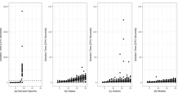
problem . . . 48 2.7. The solution times required to solve the non-adaptive problem using the

WSU and MIP solution methods for 100 random instances of various

prob-lem sizes . . . 55 2.8. An illustration of the state and action spaces of the CVD management MDP 58 2.9. The performance of the policies generated using the WSU approximation

algorithm in the CVD MMDP . . . 61 2.10. Medication usage in the CVD management MMDP . . . 65 3.1. An illustration of the machine maintenance problem with one repair option 84 3.2. Samples from the Dirichlet distributions used in the machine repair case

study . . . 85 4.1. An illustration of how an MMDP would be projected on an (s, a)-rectangular

ambiguity set. . . 101 4.2. Samples from the Dirichlet distributions used in the machine repair case

(10)

4.3. An illustration of the ambiguity-aware MMDP policies for the various for-mulations of the machine maintenance MMDP when the models are

gen-erated from a Dirichlet distribution with a concentration parameter of 10. 106 4.4. An illustration of the ambiguity-aware MMDP policies for the various

for-mulations of the machine maintenance MMDP when the models are

gen-erated from a Dirichlet distribution with a concentration parameter of 20. 107 4.5. An illustration of the ambiguity-aware MMDP policies for the various

for-mulations of the machine maintenance MMDP when the models are

gen-erated from a Dirichlet distribution with a concentration parameter of 100. 108 4.6. CDFs for the value functions and regret corresponding to each of the

MMDP policies in the machine maintenance MMDP. . . 111 4.7. A comparison of the MMDP policies as evaluated in the (s, a)-rect-MMDP,

MVP-MMDP, and the values in their corresponding worst-case models. . 112 4.8. A stylized diagram of possible transitions in the CVD MMDP . . . 115 4.9. Histograms of samples from the Dirichlet distributions used in the CVD

MMDP . . . 119 4.10. An illustration of the ambiguity-aware MMDP policies for the various

formulations of the cardiovascular disease management MMDP when the

Dirichlet distribution has a concentration parameter of α= 10 . . . 122 4.11. An illustration of the ambiguity-aware MMDP policies for the various

formulations of the cardiovascular disease management MMDP when the

Dirichlet distribution has a concentration parameter of α= 20 . . . 123 4.12. CDFs for the value functions and regret corresponding to each of the

MMDP policies in the MMDP for CVD management. . . 125 4.13. A comparison of the MMDP policies as evaluated in the MVP, the (s, a

(11)

List of Tables

2.1. Summary of the main properties and solution methods related to the

non-adaptive and non-adaptive problems for multi-model MDPs (MMDPs) . . . . 21 2.2. An explicit enumeration of the weighted value under every possible

deter-ministic policy for the non-adaptive weighted value problem. . . 49 2.3. The solution times for the CVD MMDP . . . 60 2.4. A comparison of WSU and nominal policies for CVD MMDP . . . 63 3.1. Measures of ambiguity and computational performance of the extensive

form, Branch-and-cut, and Branch-and-bound on the machine mainte-nance MMDP for various values of the concentration parameter, α, and

number of models |M| . . . 86 4.1. A summary of the formulations of the MMDP considered. . . 92 4.2. A summary of the complexity results related to ambiguity-aware MMDPs 94 4.3. A summary of the solution methods used to solve ambiguity-aware MMDPs 95

(12)

List of Acronyms

ACC/AHA American College of Cardiology/ American Heart Association. B&B branch-and-bound.

B&C branch-and-cut. BFS best-first search. BrFS breadth-first search.

CDF cumulative distribution function. CHD coronary heart disease.

CMDP contextual Markov decision process. CVD cardiovascular disease.

DFS depth-first search. DM decision maker.

EVPI expected value of perfect information. FHS Framingham Heart Study.

FIT fecal immunochemical testing. HDL high density lipoprotein. LP linear program.

(13)

MDP Markov decision process. MIP mixed-integer program.

MMDP multi-model Markov decision process. MVP mean value problem.

PercOpt percentile optimization. POMDP partially-observable MDP. QALY quality-adjusted life year. SBP systolic blood pressure. SOS special ordered set. TC total cholesterol.

VSS value of the stochastic solution. WSU Weight-Select-Update.

(14)

Abstract

Stochastic dynamic optimization methods are powerful mathematical tools for informing sequential decision-making in environments where the outcomes of decisions are uncertain. For instance, the Markov decision process has found success in many application areas that involve sequential decision-making under uncertainty, including the evaluation and design of treatment and screening protocols for medical decision making. However, the useful-ness of these models is only as good as the data used to parameterize them, and multiple competing data sources are common in many application areas, including medicine. Unfor-tunately, the recommendations that result from the optimization process can be sensitive to the data used and thus, susceptible to the impacts of ambiguity in the choices regarding the model’s construction.

To address the issue of ambiguity in Markov decision processes, we introduce the multi-model Markov decision process (MMDP) which generalizes a standard Markov decision process (MDP) by allowing for multiple models of the rewards and transition probabilities. Solution of the MMDP generates a single policy that considers the performance of the policy with respect to the diﬀerent models of the parameters. This approach allows for the decision maker (DM) to explicitly trade oﬀ conflicting sources of data. In this thesis, we study this problem in three parts.

In the first part, we study theweighted value problem (WVP)in which the DM’s objective is to find a single policy that maximizes the weighted value of expected rewards in each model. We identify two important variants of this problem: the non-adaptive WVP in which the DM must specify the decision-making strategy before the outcome of ambiguity is observed and theadaptive WVPin which the DM is allowed to adapt to the outcomes of ambiguity. We study the structural properties of these problems and establish important connections to partially-observable MDPs (POMDPs) and stochastic integer programs. To solve these problems, we develop exact methods and fast approximation methods supported by error bounds. Finally, we illustrate the eﬀectiveness and the scalability of our approach

(15)

using a case study in preventative blood pressure and cholesterol management that accounts for conflicting published cardiovascular risk models.

In the second part, we leverage the special structure of the non-adaptive WVP to de-sign exact decomposition methods for solving MMDPs with a larger number of models. We present a branch-and-cut (B&C) approach to solve a mixed-integer program (MIP) formulation of the problem and a custom branch-and-bound (B&B) approach. Both ap-proaches leverage the decomposable structure of the problem and allows for the solution of MMDPs with a larger number of models. Numerical experiments show that a customized implementation of B&B significantly outperforms B&C.

In the third part, we extend the MMDP beyond the WVP to consider other objective functions that are sensitive to the ambiguity arising from the existence of multiple mod-els. We summarize existing ambiguity-aware formulations and provide modifications to the B&B procedure to solve these alternate formulations. We compare the solution of the MMDP under these alternative objective functions and compare to a tractable approach for handling ambiguity in the transition probability matrices for MDPs that relies on an assumption that models can be selected independently for diﬀerent points in the planning horizon. We compare these formulations in two case studies related to MDPs of deterio-rating systems. We show that the solution to the mean value problem (MVP), wherein all parameters take on their mean values, can perform quite well with respect to several measures of performance under ambiguity. We also show that a common method for ad-dressing ambiguity can lead to overly aggressive actions. We illustrate that it is possible for this classical approach to perform worse than the policy resulting from the MVP in terms of performance in each MMDP model.

In summary, in this dissertation we present new methods for sequential decision-making under uncertainty in the presence of ambiguity. We consider the problem through the lens of MDPs and stochastic programming and present results for measuring the impact of ambiguity on performance. We analyze alternative forms of the problems, describe the complexity of the problems, develop solution methods, and identify properties of the op-timal solutions that provide insight into the eﬀects of ambiguity on opop-timal policies. Our findings suggest that model averaging may be a suitable approach when the ambiguous parameters are closely concentrated around their mean values. However, in other settings, the impact of ambiguity is much more substantial and our methods outperform the more traditional approaches in these settings. Although we illustrate our methods on decision-making for medical treatment and machine maintenance, the methods we present in this

(16)

thesis can be applied to other domains in which optimal sequential decision-making uncer-tainty is clouded by ambiguity.

(17)

Chapter 1 Introduction

Throughout our personal and professional lives, we all must make decisions. Often times, determining the best decisions can be quite complicated because we must weigh the short-term consequences of these decisions against the long-short-term consequences. Decisions can be further complicated because the future is clouded by uncertainty. While we are able to in-fluence what happens in the future, we are unable to completely control our destiny due to inherent randomness. Although many decision makers (DMs) wish to make decisions that best position themselves to achieve their future goals, these factors can leave DMs unsure how best to proceed. The field of stochastic dynamic optimization describes mathematical tools that can be used to inform decision-making in these challenging settings. Optimiza-tion describes the field of mathematics focused on selecting the best set of decisions among the alternatives as measured by an objective function. Dynamic optimization describes the methods used when these decisions are made sequentially over time such that deci-sions made now may influence the decideci-sions made in the future. Stochastic optimization describes the decision-making setting in which the environment evolves in part due to ran-domness and in part due to the decisions made. Hence, stochastic dynamic optimization can be succinctly described as the field of sequential decision-making under uncertainty. This field has been quite well-studied and has found success in helping DMs in many areas including inventory management, machine maintenance, finance, and healthcare [10, 56]

While standard stochastic dynamic optimization methods are powerful for informing sequential decision-making under uncertainty, these methods have often ignored another layer of uncertainty that faces DMs: the lack of knowledge around the uncertain environ-ment. That is, we may use mathematical models to represent uncertainty, but often times we do not know the best mathematical model to represent the uncertainty in how a system

(18)

evolves over time, which can limit the usefulness of the resulting recommendations. To understand how this limitation can impact decision-making, consider that we are oﬀered a bet that depends on the outcome of a flip of a weighted coin. If we know how the coin is weighted, we can evaluate the expected benefit of each outcome and weigh that outcome with how likely it is to occur. However, if the weight of the coin is unknown, our decision becomes much more diﬃcult as we no longer are certain about what the best mathematical model is to help us guide our decisions. For clarity, throughout this thesis, we will refer to uncertainty as the imperfect information about the future which can be characterized via a mathematical model. We refer to ambiguity as the imperfect information about the mathematical model itself.

In this thesis, we consider the impact of ambiguity on a particular stochastic dynamic optimization method: the Markov decision process (MDP). The MDP is a mathematical model of sequential decision-making under uncertainty, which models the decision-making process as a controlled stochastic system. The MDP generalizes a Markov chain wherein the DM can take actions to influence the transition dynamics of the system. Standard methods allow for the MDP to be solved quickly and provide the DM with a set of actions that maximize the expected value over the planning horizon. Unfortunately, the optimal course of action, as prescribed by the optimization of the MDP, is sensitive to the probabilities that describe the likelihood of transitions that characterize the stochastic process of the system’s progression through the possible states.

In the operations research literature, ambiguity in model parameters is typically handled through one of two paradigms: robust optimization and stochastic optimization. Robust optimization handles ambiguity in the parameters by assuming that the parameters are allowed to vary within anambiguity set(sometimes called an uncertainty set). The typical robust optimization approach is to determine the decisions that will perform the best under the worst-case realization of those parameters when they are allowed to vary within the ambiguity set. Robust optimization has been the standard approach for handling ambiguity in the transition matrices of MDPs. However, the literature has shown that the ambiguity sets require special structure in order to be solved quickly and relaxing this assumption can cause the resulting problems to become computationally intractable.

In this thesis, we present new results about ambiguity in MDPs through a stochastic optimization lens. In stochastic optimization, ambiguous parameters are typically modeled as random variables. In many cases, the ambiguous parameters are modeled as discrete random variables with finite support. When this is the case, the realization of these

(19)

parameters can be viewed as possible scenarios under which the system might operate. We will consider ambiguity in MDPs by allowing the transition probability and reward parameters of the MDP to be one of a finite set of models.

The theoretical contributions of this thesis were motivated by a specific application of MDPs to cardiovascular disease (CVD) management. The management of CVD is characterized by a series of sequential decisions regarding the best way to treat a patient. If a patient’s blood pressure and cholesterol levels are left uncontrolled, the patient is at higher risk of having a serious health event, such as a heart attack or stroke. Therefore, over the course of a patient’s adult life, it is suggested that a patient visit their doctor who can observe their blood pressure and cholesterol levels and help the patient make decisions regarding their health. Although lifestyle modifications are typically suggested as the first measure to lower blood pressure and cholesterol, they are frequently ineffective due to challenges associated with maintaining behavioral interventions. Thus, many US adults rely on medications to lower these risk factors which in turn lowers their risk of having a heart attack and stroke. Therefore, it is left to the doctor to make a difficult set of trade-offs. One must weigh the long-term benefit of starting a medication, which lowers a patient’s risk of having an adverse health event, with the immediate costs of starting a medication, such as the side effects and monetary costs incurred when taking the medication. However conflicting recommendations that can result from multiple reasonable models of a patient’s risk leading to ambiguity in the best course of treatment.

Summary of major contributions. In this thesis, we present methods for sequential decision-making under uncertainty in the presence of ambiguity. We summarize the main contributions from each chapter below.

Chapter 2 presents a new framework for addressing ambiguity in MDPs, which we refer to as the multi-model Markov decision process (MMDP). The main contributions of Chapter 2 are as follows:

• New Method for Handling Parameter Ambiguity in MDPs. An MMDP generalizes an MDP to allow for multiple models of the transition probabilities and rewards, each defined on a common state space and action space. In this model formulation, the places a weight on each of the models and seeks to find a single policy that will maximize the weighted value function.

• Optimal Policies for Two Cases of MMDPs. It is well-known that for standard MDPs, optimal actions are independent of past realized states and actions; optimal

(20)

policies are history independent. We show that, in general, optimal policies for MMDPs may actually be history dependent, making MMDPs more challenging to solve. With the aim of designing policies that are easily translated to practice, we distinguish between two important variants: 1) a case where the DM is limited to policies determined by the current state of the system, which we refer to as the

non-adaptive MMDP, and 2) a more general case in which the DM attempts to find an optimal history-dependent policy based on all previously observed information, which we refer to as theadaptive MMDP.

• Exact and Approximate Solution Methods. For medical decision making, the non-adaptive problem is more relevant due to its simplicity and is our primary focus. Un-fortunately, the well-known value iteration algorithm for MDPs cannot solve MMDPs to optimality. Fortunately, we are able to formulate a mixed-integer program (MIP) that produces optimal policies. We first test this method on randomly generated problem instances and find that even small instances are diﬃcult to solve; moreover, we find that the diﬀerences in objective values between the solutions of the adap-tive and the non-adapadap-tive problems are small at best. For larger problem instances though, as one might find in medical decision making applications, models are com-putationally intractable. Therefore, we introduce a fast approximation algorithm based on backwards recursion that we refer to as the Weight-Select-Update (WSU).

• Implications for CVD Management. We establish the eﬀectiveness and scalability of this new modeling approach using a case study that addresses ambiguity in the context of preventive treatment of CVD for patients with type 2 diabetes. Our study demonstrates the ability of MMDPs to blend the information of multiple competing medical studies and directly meet the challenge of designing policies that are easily translated to practice while mitigating the impact of ambiguity that arising from the existence of multiple conflicting models.

Chapter 3 expands upon the exact solution methods for the non-adaptive weighted value problem discussed on Chapter 2, which was shown to be NP-hard. We improve these exact solution methods in Chapter 3. The main contributions of Chapter 3 are:

• Decomposition Methods. In this chapter, we present two decomposition methods that leverage the decomposable structure of the problem and allow for the solution of larger MMDPs. We present a branch-and-cut (B&C) algorithm for solving the

(21)

MIP formulation of the MMDP presented in Chapter 2, as well as a customized branch-and-bound (B&B) approach which begins by relaxing the requirement that each model of the MMDP must operate under the same policy treats and subsequently adds requirements that the policies must match in certain states of the system and times during the planning horizon.

• Computational comparison. We present numerical experiments that compare the time to solve the MMDP using the following three exact solution methods: solving the extensive form of the MIP directly, solving the MIP via B&C, and solving the MMDP using the customized B&B approach. We show that the B&B algorithm outperforms the methods based on the MIP formulation of the MMDP.

• Numerical study of the impacts of ambiguity. Because we are able to solve larger MMDPs, we are able to present an analysis of the impact of ambiguity in model parameters on the resulting recommendations from the MMDP. We find that when the models’ parameters are concentrated around their mean value, the solution of the mean value problem (MVP), wherein all parameters take on their mean values, provides a near-optimal solution to the weighted value problem in many cases. How-ever, when the models’ parameters are distributed further from their mean, there is more benefit to solving the weighted value problem.

Chapter 4 extends the model presented in Chapter 2 to reflect other risk-preferences to-wards ambiguity represented as a finite number of scenarios, as in the MMDP.

• B&B for alternative risk preferences. We compile recent advances in MMDPs that consider alternative risk preferences towards ambiguity. We show that these formu-lations are also solved with minor modifications to the B&B procedure presented in Chapter 3.

• Numerical study on the mitigation of ambiguity. The flexibility of the B&B proce-dure to incorporate other risk preferences and its success in solving moderately-sized MMDPs allows us to perform one of the first analyses comparing various proposed methods in terms of their eﬀectiveness in mitigating the impact of ambiguity on finite-horizon MDPs. We compare alternative formulations of the MMDP and eval-uate the resulting policies in terms of their performance on several metrics. These alternative formulations show that the MVP does well on a variety of metrics for

(22)

finite-horizon MDPs. We also show that the DM should use caution when using methods described by earlier work if the assumptions required do not hold, as these can produce policies that perform worse than simply using the MVP’s policy. The novel contributions of this thesis are embodied in Chapters 2-4, which present the findings described above. The thesis concludes with Chapter 5 which presents a summary of the most important findings and an outline of opportunities for future research that stem from this work.

(23)

Chapter 2 Multi-model Markov Decision Processes

2.1. Introduction

The MDP is a mathematical framework for sequential decision making under uncertainty that has informed decision making in a variety of application areas including inventory control, scheduling, finance, and medicine [10, 56]. MDPs generalize Markov chains in that a DM can take actions to influence the rewards and transition dynamics of the system. When the transition dynamics and rewards are known with certainty, standard dynamic programming methods can be used to find an optimal policy, or set of decisions, that will maximize the expected rewards over the planning horizon.

Unfortunately, the estimates of rewards and transition dynamics used to parameterize the MDPs are often imprecise and lead the DM to make decisions that do not perform well with respect to the true system. The imprecision in the estimates arises because these values are typically obtained from observational data or from multiple external sources. When the policy found via an optimization process using the estimates is evaluated under the true parameters, the performance can be worse than anticipated [46]. This motivates the need for MDPs that account for this ambiguity in the MDP parameters.

In this chapter, we are motivated by situations in which the DM relies on external sources to parameterize the model but has multiple credible choices which provide potentially conflicting estimates of the parameters. In this situation, the DM may be grappling with the following questions: Which source should be used to parameterize the model? What are the potential implications of using one source over another? To address these questions, we propose a new method that allows the DM to simultaneously consider multiple models of the MDP parameters and create a policy that balances the performance while being no

(24)

more complicated than an optimal policy for an MDP that only considers one model of the parameters.

2.1.1. Applications to medical decision making

We are motivated by medical applications for which Markov chains are among the most commonly used stochastic models for decision making. A keyword search of the US Library of Medicine Database using PubMed from 2007 to 2017 reveals more than 7,500 articles on the topic of Markov chains. Generalizing Markov chains to include decisions and rewards, MDPs are useful for designing optimal treatment and screening protocols, and have found success doing so for a number of important diseases; e.g., end-stage liver disease [2], HIV [64], breast cancer [4], and diabetes [47].

Despite the potential of MDPs to inform medical decision making, the utility of these models is often at the mercy of the data available to parameterize the models. The tran-sition dynamics in medical decision making models are often parameterized using longi-tudinal observational patient data and/or results from the medical literature. However, longitudinal data are often limited due to the cost of acquisition, and therefore transition probability estimates are subject to statistical uncertainty. Challenges also arise in control-ling observational patient data for bias and often there are unsettled conflicts in the results from diﬀerent clinical studies; see Mount Hood 4 Modeling Group [51], Etzioni et al. [22], and Mandelblatt et al. [44] for examples in the contexts of breast cancer, prostate cancer, and diabetes, respectively.

A specific example, and one that we will explore in detail, is in the context of CVD for which cardiovascular risk calculators estimate the probability of a major cardiovascular event, such as a heart attack or stroke. There are multiple well-established risk calcula-tors in the clinical literature that could be used to estimate these transition probabilities, including the American College of Cardiology/ American Heart Association (ACC/AHA) Risk Estimator [27] and the risk equations resulting from the Framingham Heart Study (FHS) [75, 76]. However, these two credible models give conflicting estimates of a patient’s risk of having a major cardiovascular event. Steimle and Denton [69] showed that the best treatment protocol for CVD is sensitive to which of these conflicting estimates are used leaving an open question as to which clinical study should be used to parameterize the model.

(25)

been recognized by others (in particular, Bertsimas, Silberholz, and Trikalinos [8]), but it has not been addressed previously in the context of MDPs. As pointed out in a report from the Cancer Intervention and Surveillance Modeling Network regarding a compara-tive modeling eﬀort for breast cancer, the authors note that “the challenge for reporting multimodel results to policymakers is to keep it (nearly) as simple as reporting one-model results, but with the understanding that it is more informative and more credible. We have not yet met this challenge” [31]. This highlights the goal of designing policies that are as easily translated to practice as those that optimize with respect to a single model, but with the robustness of policies that consider multiple models. The primary contribution of our work is meeting this challenge for MDPs.

The general problem of coping with multiple (potentially valid) choices of data for med-ical decision making motivates the following more general research questions: How can we improve stochastic dynamic optimization methods to account for parameter ambiguity in MDPs? Further, how much benefit is there to mitigating the eﬀects of ambiguity?

2.1.2. Contributions

In this chapter, we present a new approach for handling parameter ambiguity in MDPs, which we refer to as the MMDP. An MMDP generalizes an MDP to allow for multiple models of the transition probabilities and rewards, each defined on a common state space and action space. In this model formulation, the DM places a weight on each of the models and seeks to find a single policy that will maximize the weighted value function. This model was proposed concurrently by Steimle, Kaufman, and Denton [70] for finite-horizon MDPs and by Buchholz and Scheftelowitsch [14] for infinite-horizon MDPs under the name of

concurrent MDPs.

It is well-known that for standard MDPs, optimal actions are independent of past realized states and actions; optimal policies are history independent. We show that, in general, optimal policies for MMDPs may actually be history dependent, making MMDPs more challenging to solve. With the aim of designing policies that are easily translated to practice, we distinguish between two important variants: 1) a case where the DM is limited to policies determined by the current state of the system, which we refer to as the non-adaptive MMDP, and 2) a more general case in which the DM attempts to find an optimal history-dependent policy based on all previously observed information, which we refer to as the MMDP. We show that the adaptive problem is a special case of a partially-observable

(26)

MDP (POMDP) that is PSPACE-hard, and we show that the non-adaptive problem is NP-hard.

For medical decision making, the non-adaptive problem is more relevant due to its sim-plicity and is our primary focus. Unfortunately, the well-known value iteration algorithm for MDPs cannot solve MMDPs to optimality. Fortunately, we are able to formulate a MIP that produces optimal policies. We first test this method on randomly generated problem instances and find that even small instances are diﬃcult to solve; moreover, we find that the diﬀerences in objective values between the solutions of the adaptive and the non-adaptive problems are small at best. For larger problem instances though, as one might find in medical decision making applications, models are computationally intractable. Therefore, we introduce a fast approximation algorithm based on backward recursion that we refer to as the WSU.

Finally, we establish the eﬀectiveness and scalability of this new modeling approach using a case study that addresses ambiguity in the context of preventive treatment of CVD for patients with type 2 diabetes. Our study demonstrates the ability of MMDPs to blend the information of multiple competing medical studies (ACC/AHA and FHS) and directly meet the challenge of designing policies that are easily translated to practice while being robust to ambiguity arising from the existence of multiple conflicting models.

2.1.3. Organization of the chapter

The remainder of this chapter is organized as follows: In Section 2.2, we provide some important background on MDPs and discuss the literature that is most related to our work. We formally define the MMDP in Section 2.3, and in Section 2.4 we present analysis of our proposed MMDP model. In Section 2.5, we discuss exact solution methods as well as fast and scalable approximation methods that exploit the model structure. We test these approximation algorithms on randomly generated problem instances and describe the results in Section 2.6. In Section 2.7, we present our case study. Finally, in Section 2.8, we summarize the most important findings from our research and discuss the limitations and opportunities for future research.

(27)

2.2. Background

In this chapter, we focus on discrete-time, finite-horizon MDPs under ambiguity. In this section, we will describe the MDP and parameter ambiguity, as well as the related work aimed at mitigating the eﬀects of ambiguity in MDPs.

2.2.1. Markov decision processes

MDPs are a common framework for modeling sequential decision-making that influences a stochastic reward process. For ease of explanation, we introduce the MDP as an interaction between an exogenous actor, nature, and the DM. The sequence of events that define the MDP are as follows: first, nature randomly selects an initial state s1 ∈ S according to the

initial distribution µ1 ∈ M(S), where M(·) denotes the set of probability measures on

the discrete set. The DM observes the state s1 ∈ S and selects an action a1 ∈ A. Then,

the DM receives a reward r1(s1, a1)∈ R and then nature selects a new state s2 ∈ S with

probability p1(s2 | s1, a1) ∈ [0,1]. This process continues whereby for any decision epoch

t∈ T ≡ {1, . . . , T}, the DM observes the statest∈ S, selects an actionat ∈ A, and receives

a rewardrt(st, st), and nature selects a new statest+1 ∈ S with probability pt(st+1 |st, at). The DM selects the last action at time T which may influence which state is observed at time T + 1 through the transition probabilities. Upon reaching sT+1 ∈ S at time T + 1,

the DM receives a terminal reward of rT+1(sT+1) ∈ R. Future rewards are discounted

at a rate of α ∈ (0,1] which accounts for the preference of rewards received now over rewards received in the future. In this chapter, we assume without loss of generality that the discount factor is already incorporated into the reward definition. We will refer to the times at which the DM selects an action as the set ofdecision epochs,T, the set of rewards asR ∈R|S×A×T |, and the set of transition probabilities as P ∈R|S×A×S×T | with elements satisfying pt(st+1 |st, at)∈ [0,1] and

∑

st+1∈Spt(st+1 |st, at) = 1, ∀t∈ T, st ∈ S, at ∈ A. Throughout the remainder of this chapter, we will use the tuple (T,S,A, R, P, µ1) to

summarize the parameters of an MDP.

The realized value of the DM’s sequence of actions is the total reward over the planning horizon:

T ∑

t=1

rt(st, at) +rT+1(sT+1). (2.1)

(28)

(2.1) with respect to the distribution defined by the transition probabilities is maximized. Thus, the DM will select the actions at each decision epoch based on some information available to her. The strategy by which the DM selects the action for each state at decision epocht∈ T is called adecision rule,πt∈Πt, and the set of decision rules over the planning horizon is called apolicy,π ∈Π.

There exist two dichotomies in the classes of policies that a DM may select from: 1) history-dependent vs. Markov, and 2) randomized vs. deterministic. History-dependent policies may consider the entire history of the MDP, ht := (s1, a1, . . . , at−1, st), when prescribing which action to select at decision epoch t ∈ T, while Markov policies only consider the current state st ∈ S when selecting an action. Randomized policies specify a probability distribution over the action set, πt(st) ∈ M(A), such that action at ∈ A will be selected with probabilityπt(at|st). Deterministic policies specify a single action to be selected with probability 1. Markov policies are a subset of history-dependent policies, and deterministic policies are a subset of randomized policies. For standard MDPs, there is guaranteed to be a Markov deterministic policy that maximizes the expectation of (2.1) [Proposition 4.4.3 in 56] which allows for eﬃcient solution methods that limit the search for optimal policies to the Markov deterministic (MD) policy class, π ∈ ΠM D. We will distinguish between history-dependent (H) and Markov (M), as well as randomized (R) and deterministic (D), using superscripts on Π. For example, ΠM R denotes the class of Markov randomized policies.

To summarize, given an MDP (T,S,A, R, P, µ1), the DM seeks to find a policy π that

maximizes the expected rewards over the planning horizon:

max π∈Π E π,P,µ1 [ _T ∑ t=1 rt(st, at) +rT+1(sT+1) ] . (2.2)

A standard MDP solution can be computed in polynomial time because the problem de-composes when the search over Π is limited to the Markov deterministic policy class, ΠM D_. We will show that this and other properties of MDPs no longer hold when parameter am-biguity is considered.

2.2.2. Parameter ambiguity and related work

MDPs are known as models of sequential decision making under uncertainty. However, this “uncertainty” refers to the imperfect information about the future state of the system

(29)

after an action has been taken due to stochasticity. The transition probability parameters are used to characterize the likelihood of these future events. For the reasons described in Section 2.1, the model parameters themselves may not be known with certainty. As a reminder, we will refer touncertainty as the imperfect information about the future which can be characterized via a set of transition probability parameters. We refer toambiguity

as the imperfect information about the transition probability parameters themselves. In this chapter, we consider a variation on MDP in which parameter ambiguity is ex-pressed through multiple models of the underlying Markov chain, and the goal of the DM is to find a policy that maximizes the weighted performance across these different mod-els. The concept of multiple models of parameters is seen in the stochastic programming literature whereby each set corresponds to a “scenario” representing a different possibility for the problem data [9]. Stochastic programming problems typically consist of multiple stages during which the DM has differing levels of information about the model parame-ters. For example, in a two-stage stochastic program, the DM selects initial actions during the first-stage before knowing which of the multiple scenarios will occur. The DM subse-quently observes which scenario is realized and takesrecourse actions in the second stage. In contrast, in MMDP, the model parameters will never be revealed to the DM.

Perhaps the most closely related research to this chapter is that of Bertsimas, Silberholz, and Trikalinos [8] who recently addressed ambiguity in simulation modeling in the context of prostate cancer screening. The authors propose solving a series of optimization problems via an iterated local search heuristic to find screening protocols that generate a Pareto optimal frontier on the dimensions of average-case and worst-case performance in a set of diﬀerent simulation models. This article identified the general problem of multiple models in medical decision making; however, they do not consider this issue in MDPs. The concept of multiple models of problem parameters in MDPs has mostly been used as a form of sensitivity analysis. For example, Craig and Sendi [17] propose bootstrapping as a way to generate multiple sets of problem parameters under which to evaluate the robustness of a policy to variation in the transition probabilities. There has been less focus on finding policies that perform well with respect to multiple models of the problem parameters in MDPs. As pointed out in a report from the Cancer Intervention and Surveillance Modeling Network regarding a comparative modeling eﬀort for breast cancer, the authors note that “the challenge for reporting multi-model results to policymakers is to keep it (nearly) as simple as reporting one-model results, but with an understanding that it is more informative and more credible. We have not yet met this challenge” [31]. This

(30)

highlights the goal of designing policies that are as easily translated to practice as those that optimize with respect to a single model, but with the robustness of policies that consider performance in multiple models.

The approach of incorporating multiple models of parameters is also seen in the rein-forcement learning literature, however the objective of the DM in these problems is different than the objective of the DM in this chapter. For example, consider what is perhaps the most closely related reinforcement learning problem: the contextual Markov decision pro-cess (CMDP) proposed by Hallak, Di Castro, and Mannor. The CMDP is essentially the same as the MMDP set-up in that one can think of the CMDP asC MDPs all defined on the same state space and action space, but with different reward and transition probability parameters. In the CMDP problem, the DM will interact with the CMDP throughout a series of episodes occurring serially in time. At the beginning of the interaction, the DM neither has any information about any of the C MDP’s parameters, nor does she know which MDP she is interacting with at the beginning of each episode. Our work differs from that of [32] in that we assume the DM has a complete characterization of each of the MDPs, but due to ambiguity the DM still does not know which MDP she is interacting with. Others have studied related problems in the setting ofmulti-task reinforcement learn-ing [13]. Our work differs from this line of research in that we are motivated by problems with shorter horizons while contextual and multi-task learning is appropriate for problems in which the planning horizon is sufficiently long to observe convergence of estimates to their true parameters based on a dynamic learning process, such as in the area of mobile health [33, 50].

Our research is distinct from the more traditional approach of mitigating parameter ambiguity in MDPs, known as robust dynamic programming, which represents parameter ambiguity through an ambiguity set formulation. The standard robust dynamic program-ming is a “max-min” approach in which the DM seeks to find a policy that maximizes the worst case performance when the transition probabilities are allowed to vary within an ambiguity set. The ambiguity set can be constructed as intervals around a point esti-mate, and the max-min approach represents that the DM is risk neutral with respect to uncertainty and risk adverse with respect to ambiguity.

A key result regarding the max-min problem is that it is tractable for instances that satisfy the (s, a)-rectangularity property [35, 52]. The (s, a)-rectangularity implies that observing the realization of a transition probability parameter gives no information about the values of other parameters for any other state-action-time triplet. Because each

(31)

param-eter value for any given state-action-time triplet is independent of the others, the problem can be decomposed so that each worst-case parameter is found via an optimization problem called theinner problem. Iyengar [35] and Nilim and El Ghaoui [52] provide algorithms for solving the max-min problem for a variety of ambiguity sets by providing polynomial-time methods for solving the corresponding inner problem.

While (s, a)-rectangular ambiguity sets are desirable from a computational perspective, they can give rise to policies that are overly-conservative because the DM must account for the possibility that parameters for each state-action-time triplet will take on their worst-case values simultaneously. Therefore, much of the research in robust dynamic program-ming has focused on ways to mitigate the eﬀects of parameter ambiguity while avoiding policies that are overly conservative by either finding non-(s, a)-rectangular ambiguity sets that are tractable for the max-min problem or optimizing with respect to another objective function usually assuming some a priori information about the model parameter [18, 30, 41, 45, 62, 74, 78].

To our knowledge, Le Tallec [40], Ahmed et al. [1], and Merakli [49], and Saghafian [59] are the only articles that have considered addressing ambiguity in the MDP parameters by using multiple discrete sets of parameters. Le Tallec introduced the concept of an MDP with “random uncertainty” wherein ambiguity is represented as a finite number of models. The author does so as a way to study the complexity of MDPs with ambiguity, but the focus is limited primarily to the complexity of such problems rather than the solution of such problems. Recently, Ahmed et al. propose sampling rewards and transition probabilities at each time step to generate a set of discrete MDPs and then seek to find one policy that minimizes the maximum regret over the set of MDPs. To do this, they formulate a MIP to approximate an optimization problem with quadratic constraints which minimizes regret. They also propose cumulative expected myopic regret as a measure of regret for which dynamic programming algorithms can be used to generate an optimal policy. The authors require that the sampled transition probabilities and rewards are stage-wise independent, satisfying the (s, a)-rectangularity property. Concurrently with our work, Merakli propose percentile optimization approach for MDPs where ambiguity is represented using a finite number of models. In the POMDP setting, Saghafian uses multiple models of the parameters to address ambiguity in transitions among the core states in a POMDP and use an objective function that weights the best-case and worst-case value-to-go across the models. This is in contrast to our work which considers the expected value-to-go among multiple models. Saghafian assumes that the best-case and

(32)

worst-case model are selected independently across decision epochs, satisfying the rectangularity assumption. In our MMDP formulation, the rectangularity assumption is not required; the objective is to find a single policy that will perform well in each of the models which may have interdependent transition probabilities across the planning horizon.

Later in this article, we will describe a case study that illustrates the effectiveness and scalability of the MMDP formulation on a medical decision making problem with parameter ambiguity in the context of prevention of cardiovascular disease. As pointed out in Section 2.1, MDPs are increasingly used for designing optimal treatment and screening protocols; however, the literature on addressing ambiguity in MDPs for medical decision making is very sparse. As mentioned previously, Bertsimas, Silberholz, and Trikalinos [8] addressed ambiguity in simulation modeling in the context of prostate cancer screening. Goh et al. [28] proposed finding the best-case and worst-case transition probability parameters for this policy when these parameters are allowed to vary within an ambiguity set. The authors assumed that this ambiguity set is a row-wise independent set that generalizes the existing row-wise ambiguity models in Iyengar [35] as well as Nilim and El Ghaoui [52]. This rectangularity assumption allows for the authors to solve a semi-infinite linear program (LP) problem efficiently. The authors apply their methods to fecal immunochemical testing (FIT) for colorectal cancer and show that, despite the ambiguity in model parameters related to FIT, this screening tool is still cost-effective relative to the most prevalent method, colonoscopy.

To our knowledge, the optimal design of medical screening and treatment protocols un-der parameter ambiguity is limited to the work of Kaufman, Schaefer, and Roberts [37], Sinha, Kotas, and Ghate [66], and Zhang, Steimle, and Denton [80]. Kaufman, Schae-fer, and Roberts [37] consider the optimal timing of living-donor liver transplantation, for which some critical health states are seldom visited historically. They use the robust MDP framework, modeling ambiguity sets as confidence regions based on relative entropy bounds. The resulting robust solutions are of a simple control-limit form that suggest transplanting sooner, when patients are healthier, than otherwise suggested by traditional MDP solu-tions based on maximum likelihood estimates of transition probabilities. Sinha, Kotas, and Ghate [66] use a robust MDP formulation for response-guided dosing decisions in which the dose-response parameter is allowed to vary within an interval ambiguity set and show that a monotone dosing policy is optimal for the robust MDP. Zhang, Steimle, and Den-ton [80] propose a robust MDP framework in which transition probabilities are confined to statistical confidence intervals. They employ a rectangularity assumption implying

(33)

inde-pendence of rows in the transition probability matrix. They assume an adversarial model in which the DM decides on a policy, and an adversary optimizes the choice of transition probabilities that minimizes expected rewards subject to an “uncertainty budget” on the choice of transition probabilities. While these articles address parameter ambiguity in the transition probabilities, they all assume an (s, a)-rectangular ambiguity set which decou-ples the ambiguity across decision epochs and states. In contrast, the MMDP formulation that we propose allows for the ambiguity in model parameters to be linked across tuples of states, actions, and decision epochs.

2.3. Multi-model Markov decision processes

In this section, we introduce the detailed mathematical formulation of the MMDP starting with the following definition:

Definition 2.1 (Multi-model Markov decision process). An MMDP is a tuple

(T,S,A,M,Λ) where T is the set of decision epochs, S and A are the state and action spaces respectively, M is the finite discrete set of models, and Λ := {λ1, . . . , λ|M|} is the

set of exogenous models weights with λm ∈ (0,1),∀m ∈ M and ∑_m_∈Mλm = 1. Each model m ∈ M is an MDP, (T,S,A, Rm_{, P}m_{, µ}m

1 ), with a unique combination of rewards,

transition probabilities, and initial distribution.

The requirement that λm ∈ (0,1) is to avoid the trivial cases: If there exists a model m ∈ M such that λm = 1, the MMDP would reduce to a standard MDP. If there exists a model m ∈ M such that λm = 0, then the MMDP would reduce to an MMDP with a smaller set of models, M \ {m}. The model weights, Λ, may be selected via expert judgment to stress the relative importance of each model, as tunable parameters which the DM can vary (as illustrated in the case study in Section 2.7), according to a probability distribution over the models, or as uninformed priors when each model is considered equally reputable (as in [8]).

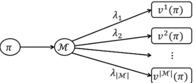
In an MMDP, the DM considers the expected rewards of the specified policy in the multiple models. The value of a policy π ∈ Π in model m ∈ M is given by its expected rewards evaluated with modelm’s parameters:

vm(π) :=Eπ,Pm,µm1 [ _T ∑ t=1 r_tm(st, at) +rTm+1(sT+1) ] .

(34)

We associate any policy,π ∈Π, for the MMDP with itsweighted value: W(π) := ∑ m∈M λmvm(π) = ∑ m∈M λmEπ,P m_,µm 1 [ _T ∑ t=1 rm_t (st, at) +rmT+1(sT+1) ] . (2.3)

Thus, we consider the weighted value problem (WVP) in which the goal of the DM is to find the policy π∈Π that maximizes the weighted value defined in (2.3):

Definition 2.2 (Weighted value problem). Given an MMDP (T,S,A,M,Λ), the WVP is defined as the problem of finding a solution to:

W∗ := max π∈Π W(π) = maxπ∈Π { ∑ m∈M λmEπ,P m_,µm 1 [ _T ∑ t=1 rm_t (st, at) +rmT+1(sT+1) ]} (2.4)

and a set of policies Π∗ :={π∗ : W(π∗) =W∗} ⊆Π that achieve the maximum in (2.4).

The WVP can be viewed as an interaction between the DM (who seeks to maximize the expected weighted value of the MMDP) and nature. In many robust formulations, nature is viewed as an adversary which represents the risk-aversion to ambiguity in model parameters. However, in the WVP, nature plays the role of a neutral counterpart to the DM. In this interaction, the DM knows the complete characterization of each of the models, and nature selects which model will be given to the DM by randomly sampling according to the probability distribution defined by Λ ∈ M(M). For a fixed model m ∈ M, there will exist an optimal policy for m that is Markov (i.e., π∗_m ∈ ΠM_{). We will focus on the} problem of finding a policy that achieves the maximum in (2.4) when Π = ΠM. We will refer to this problem as thenon-adaptive problem because we are enforcing that the DM’s policy be based solely on the current state, and she cannot adjust her strategy based on what sequences of states she has observed. As we will show, unlike traditional MDPs, the restriction to ΠM _{may not lead to an overall optimal solution. For completeness,} we will also describe an extension, called the adaptive problem, where the DM can utilize information about the history of observed states, however this extension is not the primary focus of this article. The evaluation of a given policy in the WVP is illustrated in Figure 2.1.

(35)

Figure 2.1: An illustration of policy evaluation in terms of weighted value, which is the objective function used to compare policies for an MMDP. The DM specifies a

policy π which is subsequently evaluated in each of the |M| models. The weighted

value of a policy π is determined by taking of the sum of this policy’s value in each

model m, vm₍_π₎_{, weighted by the corresponding model weight} _λ

m.

2.3.1. The non-adaptive problem

Thenon-adaptive problem for MDPs is an interaction between nature and the DM. In this interaction, the DM specifies a Markov policy, π ∈ ΠM, a priori. In this case, the policy is composed of actions based only on the current state at each decision epoch. Therefore the policy is a distribution over the actions: π = {πt(st) = (πt(1 | st), . . . , πt(|A| | st)) ∈

M(A) : at ∈ A, st ∈ S, t ∈ T }. In this policy, πt(at | st) is the probability of selecting

action at ∈ A if the MMDP is in state st ∈ S at time t ∈ T. Then, after the DM has specified the policy, nature randomly selects model m ∈ M with probability λm. Now, nature selectss1 ∈ S according to the initial distributionµm1 ∈M(S), and the DM selects

an action, a1 ∈ A, according to the pre-specified distribution π1(s1) ∈ M(A). Then,

nature selects the next state s2 ∈ S according to pm1 (·|s1, a1) ∈ M(S). The interaction

carries on in this way where the DM selects actions according to the pre-specified policy,π, and nature selects the next state according to the distribution given by the corresponding row of the transition probability matrix. From this point of view, it is easy to see that under a fixed policy, the dynamics of the stochastic process follow a Markov chain. Policy evaluation then is straightforward; one can use backward recursion. While policy evaluation is similar for MMDPs as compared to standard MDPs, policy optimization is much more challenging for MMDPs. For example, value iteration, a well-known solution technique for MDPs, does not apply to MMDPs where actions are coupled across models.

(36)

2.3.2. The adaptive problem

The adaptive problem generalizes the non-adaptive problem to allow the DM to utilize realizations of the states to adjust her strategy. In this problem, nature and the DM interact sequentially where the DM gets new information in each decision epoch of the MMDP and the DM is allowed to utilize the realizations of the states to infer information about the ambiguous problem parameters when selecting her future actions. In this setting, nature begins the interaction by selecting a model,m∈ M, according to the distribution Λ, and the model selected is not known to the DM. Nature then selects an initial states1 ∈ S

according to the model’s initial distribution,µm

1 . Next, the DM observes the state,s1, and

makes her move by selecting an action, a1 ∈ A. At this point, nature randomly samples

the next state, s2 ∈ S, according to the distribution given by pm1 (·|s1, a1) ∈ M(S). The

interaction continues by alternating between the DM (who observes the state and selects an action) and nature (who selects the next state according to the distribution defined by the corresponding row of the transition probability matrix).

In the adaptive problem, the DM considers the current state of the MMDP along with information about all previous states observed and actions taken. Because the history is available to the DM, the DM may be able to infer which model is most likely to correctly characterize the behavior of nature which the DM is observing. As we will formally prove later, in this context the DM will specify a history-dependent policy in general, π =

{πt(ht) :ht∈ S × A ×. . .× A × S, t∈ T }.

2.4. Analysis of MMDPs

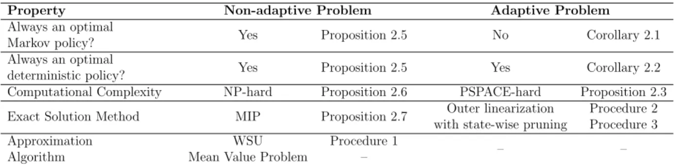
In this section, we will analyze the WVP as defined in (2.4). For both the adaptive and non-adaptive problems, we will describe the classes of policies that achieve the optimal weighted value, the complexity of solving the problem, and related problems that may provide insights into promising solution methods. These results and solution methods are summarized in Table 2.1.

2.4.1. General properties of the weighted value problem

In both the adaptive and non-adaptive problems, nature is confined to the same set of rules. However, the set of strategies available to the DM in the non-adaptive problem is

(37)

Property Non-adaptive Problem Adaptive Problem Always an optimal

Markov policy? Yes Proposition 2.5 No Corollary 2.1

Always an optimal

deterministic policy? Yes Proposition 2.5 Yes Corollary 2.2

Computational Complexity NP-hard Proposition 2.6 PSPACE-hard Proposition 2.3

Exact Solution Method MIP Proposition 2.7 Outer linearization

with state-wise pruning

Procedure 2 Procedure 3 Approximation

Algorithm

WSU Mean Value Problem

Procedure 1

– – –

Table 2.1: Summary of the main properties and solution methods related to the non-adaptive and non-adaptive problems for MMDPs. Solution methods with dashed entries are not discussed in this thesis.

just a subset of the strategies available in the adaptive problem. Therefore, ifW_N∗ andW_A∗ are the best expected values that the DM can achieve in the non-adaptive and adaptive problems, respectively, then it follows thatW_N∗ ≤W_A∗.

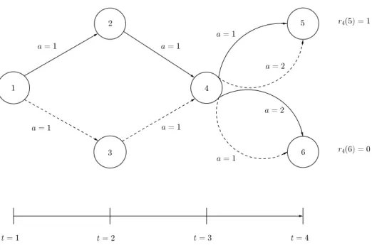
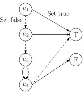
Proposition 2.1. W_N∗ ≤W_A∗. Moreover, the inequality may be strict. Proof. Consider the MMDP illustrated in Figure 2.2.

First, we describe the decision epochs, states, rewards, and actions for this MMDP. This MMDP is defined for 3 decision epochs where state 1 is the only possible state for decision epoch 1, states 2 and 3 are the states for decision epoch 2, and state 4 is the only state reachable in decision epoch 3. States 5 and 6 are terminal states. This MMDP has two models M ={1,2}. For each model, the only non-zero reward is received upon reaching the terminal state 5. In states 1, 2, and 3, the DM only has one choice of actiona= 1. In state 4, the DM can select between actiona = 1 anda= 2.

Now we will describe the transition probabilities for each model. Each line represents a transition that happens with probability one when the corresponding action is selected. Solid lines correspond to transitions for model m = 1 and dashed lines correspond to transitions for model m= 2.

Since state 4 is the only state in which there is a choice of action, we define the possible policies selecting an action in this state. Consider the adaptive problem for this MMDP. The optimal decision rule for state 4 will depend on the state observed at time t = 2: If the history of the MMDP is (s1 = 1, a1 = 1, s2 = 2, a2 = 1), then select action 1, otherwise

select action 2. In model 1, the only way to reach state 4 is through state 2. Upon observing this sample path, the policy prescribes taking action 1 which will lead to a transition to state 5 and thus a reward of 1 will be received. On the other hand, in model 2, the only

(38)

way to reach state 4 is through state 3. Therefore, the policy will always prescribe taking action 2 in model 2 which leads to state 5 with probability 1. This means that evaluating this policy in model 1 gives an expected value of 1 and evaluating this policy in model 2 gives an expected value of 1. Therefore, for any given weightsλ, this policy has a weighted value of W_A∗ = 1.

Now, consider the non-adaptive problem for the MMDP. Before the DM can observe the state at time t = 2, she must specify a decision rule to be taken in state 4. For state 4, there are two options: select action 1 or select action 2. Letqbe the probability of selecting action 1. If action 1 is selected, this will give an expected value of 1 in model 1 and an expected value of 0 in model 2, which produces a weighted value of λ1. Analogously, if

action 2 is selected, the weighted value in the MMDP will beλ2. Thus, the optimal policy

for the non-adaptive problem gives a weighted value of maxq∈[0,1]{qλ1,(1−q)λ2}which will

be exactly max{λ1, λ2}.

This means that for any choice of λ such that λ1 < 1 and λ2 < 1, the MMDP has

W_N∗ = max{λ1, λ2}<1 =WA∗. In this MMDP, there does not exist a Markov policy that is optimal for the adaptive problem.

Corollary 2.1. It is possible that there are no optimal policies that are Markovian for the adaptive problem.

The results of Proposition 2.1 and Corollary 2.1 mean that the DM may benefit from being able to recall the history of the MMDP. This history allows for the DM to infer which model is most likely, conditional on the observed sample path and tailor the future actions to reflect this changing belief about nature’s choice of model. Therefore, the DM must search for policies within the history-dependent policy class to find an optimal solution to the adaptive MMDP. These results establish that the adaptive problem does not reduce to the non-adaptive problem in general. For this reason, we separate the analysis for the adaptive and non-adaptive problems.

2.4.2. Analysis of the adaptive problem

We begin by establishing an important connection between the adaptive problem and the POMDP [67]:

(39)

Figure 2.2: An example of an MMDP with WA > WN. The MMDP shown has

six states, two actions, and two models. Each arrow represents a transition that occurs with probability 1 for the corresponding action labeling the arrow. Solid lines

represent transitions in model 1 and dashed lines represent transitions in model 2.

There are no intermediate rewards in this MMDP, but there is a terminal reward