remote sensing
ArticleMulti-Source and Multi-Temporal Image Fusion on
Hypercomplex Bases
Andreas Schmitt1,* , Anna Wendleder2, Rüdiger Kleynmans1, Maximilian Hell1, Achim Roth2and Stefan Hinz3
1 Munich University of Applied Sciences, Geoinformatics Department, Karlstraße 6, D-80333 Munich,
Germany; [email protected] (R.K.); [email protected] (M.H.)
2 German Aerospace Center (DLR), Earth Observation Center (EOC), Oberpfaffenhofen, D-82234 Weßling,
Germany; [email protected] (A.W.); [email protected] (A.R.)
3 Karlsruhe Institute of Technology (KIT), Institute of Photogrammetry and Remote Sensing (IPF), Englerstr. 7,
D-76131 Karlsruhe, Germany; [email protected]
* Correspondence: [email protected]; Tel.: +49-89-1265-2416
Received: 15 January 2020; Accepted: 10 March 2020; Published: 14 March 2020
Abstract:This article spanned a new, consistent framework for production, archiving, and provision of analysis ready data (ARD) from multi-source and multi-temporal satellite acquisitions and an subsequent image fusion. The core of the image fusion was an orthogonal transform of the reflectance channels from optical sensors on hypercomplex bases delivered in Kennaugh-like elements, which are well-known from polarimetric radar. In this way, SAR and Optics could be fused to one image data set sharing the characteristics of both: the sharpness of Optics and the texture of SAR. The special properties of Kennaugh elements regarding their scaling—linear, logarithmic, normalized—applied likewise to the new elements and guaranteed their robustness towards noise, radiometric sub-sampling, and therewith data compression. This study combined Sentinel-1 and Sentinel-2 on an Octonion basis as well as Sentinel-2 and ALOS-PALSAR-2 on a Sedenion basis. The validation using signatures of typical land cover classes showed that the efficient archiving in 4 bit images still guaranteed an accuracy over 90% in the class assignment. Due to the stability of the resulting class signatures, the fuzziness to be caught by Machine Learning Algorithms was minimized at the same time. Thus, this methodology was predestined to act as new standard for ARD remote sensing data with an subsequent image fusion processed in so-called data cubes.
Keywords:Kennaugh framework; quaternion; hypercomplex bases; image fusion; time series; change detection; SAR sharpening; data cube; analysis ready data; efficient archiving
1. Introduction
The introduction addresses the necessity for Analysis Ready Data (ARD), presents the Multi-SAR System, an evaluated framework for the production of polarimetric ARD data, and how the Multi-SAR System is expanded with a new approach for image fusion for optical and SAR data. Finally, we formulates the research questions which will be answered in the following.
1.1. Necessity for Analysis Ready Data
Earth Observation (EO) is turning more and more to ‘Big Earth Data’ [1]. By the end of 2018, the Copernicus Sentinel products had a total data volume of 10 PiB with a daily average growth of 15 TiB in November 2018 [2]. The complexity of data processing, computational power, and storage increases with the data volume. This means that even sophisticated users of EO data invest more time and effort into data preparation than into data interpretation. The idea is to support EO users to transform the
immense amounts of data into useful information and decision-ready products [3]. This challenge can be met with the provision of pre-processed EO data to a minimum set of requirements and their organization in a standardized, consistent, and transparent manner. It requires the possibility of an immediate analysis without additionally user effort, interoperability, and processing time as well as open and easy data access. The specifications are regulated within the Committee on Earth Observation Satellites (CEOS) for ARD [4]. ARD products representing surface reflectance are commonly used and their custom pre-processing workflow and provision is already standardized. Since 2008, the United States Geological Survey (USGS) provides the Landsat data asL1Tanalysis-ready products in a single, universally accessible, centralized global archive [5]. The focus of the Swiss Data Cube (SDC) is a consistent and comparable data processing and storage of different sensors. Therefore, they use the same framework for data discovery, downloading, and processing of Landsat as well as of Sentinel-2 ARD products [3,6]. The provision of ARD products representing radar backscatter started with the continuous and global coverage of Sentinel-1 imagery. The cloud based platform of Google Earth Engine provides processed Level-1 Ground Range Detected (GRD) Sentinel-1 data. The pre-processing contains border and thermal noise removal, radiometric and geometric calibration using Shuttle Radar Topography (SRTM) and Advanced Spaceborne Thermal Emission and Reflection Radiometer (ASTER) Digital Elevation Model (DEM), and conversion to decibel. It is implemented by the Sentinel Toolbox and allows a subsequent processing in Python and JavaScript languages [7]. Truckenbrodt et al. [8] analysed the capability of possible software solutions like the Sentinel Application Platform (SNAP) and GAMMA for the automatic production of Sentinel-1 ground range detected ARD products. He concluded that SNAP is a convenient and user-friendly graphical user interface and additionally, it is open source. Anyway, the error messages were difficult to interpret without prior knowledge and especially the complex Java structure complicates error search. The basic command line interface of licensed GAMMA required experiences in application and development of new workflows. Therefore, it was very robust and fast. The analyses of Ticehurst et al. [9] went beyond the usage of Sentinel-1 radar backscatter data and involved equally polarimetric radar data. She developed ARD products from SAR including normalized radar backscatter (γ0), eigenvector-based dual-polarization decomposition,
and interferometric coherence based on SNAP. Her feasibility study showed a good agreement between SNAP and GAMMA with minor systematic geometric and radiometric differences which can be neglected.
The above mentioned backscatter ARD products bases mostly on Sentinel-1 GRD data. Though, CEOS demands Level-1 Single Look Complex (SLC) ARD products in order to exploit similarly the polarimetric information. This requires a standardized provision of polarimetric radar ARD data including speckle filtering, polarimetric decomposition, and normalization of the data in order to reduce their storage demand [10]. We present the Multi-SAR System, an evaluated framework for the production of polarimetric ARD data. The Multi-SAR System contains ortho-rectification, Kennaugh decomposition, multi-looking, radiometric calibration, image enhancement using the multi-scale multi-looking (MSML) approach or Schmittlets, and normalization based on hyperbolic tangent function for the final (almost) lossless data compression according to References [11,12]. The system can be used for the processing of all SAR data in level 1 (focused, slant range, single-look, complex) independent of their geometric, radiometric, and polarimetric resolution. Its main benefit is the usage of the same workflow and the same parameter configuration file independent of the different SAR input data formats and interfaces. The final result is a SAR image in level 2 represented in a consistent ARD format. It is implemented at the German Remote Sensing Data Center (DFD) within the German Aerospace Center (DLR) at Oberpfaffenhofen.
1.2. Applications Based on Multi-SAR System
With respect to the preprocessing of SAR images acquired by different sensors in different modes a first idea how to establish a consistent frame for the ARD provision was mentioned in Reference [13], where the Kennaugh elements were chosen to perform a robust change detection
on wetlands. Already two years later, the normalized Kennaugh elements were introduced as a consistent frame for the fusion of multi-sensor and multi-polarized SAR data allowing for simple data analysis with standard and open-source software, effective data compression, and even change detection in combination with advanced locally adaptive filtering techniques [11]. Refining these filtering techniques by multi-directional kernels led to the Schmittlet approach that even enabled the analysis of image texture in the best available (total) intensity image [12]. The change detection capability was used for mapping wind throw areas in mid-European forests from TerraSAR-X images [14]. The usefulness of the normalized Kennaugh elements in the context of wetland remote sensing especially in semi-arid regions was proven several times using TerraSAR-X, RADARSAT-2, and even archived data of RADARSAT-1 and ENVISAT-ASAR [15–17]. Due to its flexibility concerning the input data, different polarization combinations could be evaluated at the same time for surface water monitoring purposes [18]. The advanced preprocessing finally enabled an almost daily estimation of the water gauge in the Forggensee in southern Germany via flooded area [19]. Furthermore, the Kennaugh decomposition was successfully utilized in coastal applications for the mapping of bivalve beds on exposed intertidal flats from dual-co-polarized TerraSAR-X data [20]. Going further north, the normalized Kennaugh elements excelled as input feature for classification of Tundra environments in northern Canada. The relation between snow depth, topography, and vegetation was studied on TerraSAR-X time series preprocessed to Kennaugh elements [21]. Even for the understanding of snow covered sea ice processes from TerraSAR-X the Kennaugh preprocessing showed up to be essential [22]. Regarding glaciered areas, the polarimetric information captured in Kennaugh elements helped to detect the supraglacial meltwater drainage on the Devon Ice Cap, Canada. Alpine glaciers were also analysed by normalized Kennaugh elements—a study evaluated the correlation between ground-based radar measurements and space-borne multi-polarized SAR images over the Vernagtferner in the Oetztaler Alps, Austria, [23], the other study evaluated time series of Sentinel-1 data over several summers in order to discriminate wet snow from firn as a first step towards a mass balance estimation from space [24]. Apart from natural landscapes the Kennaugh elements provided a valuable input for the mapping of slums from polarimetric SAR data [25]. In combination with the Schmittlet index and a highly sophisticated, multi-scale classification approach—called histogram classification—the discrimination of formal from informal settlements by multi-aspect SAR images became feasible [26]. The histogram classification which bases on the similarity measure for the comparison of two discrete local histograms was further studied for typical land cover classification based on reflectance data only [27]. Recently, a very promising new approach was published how to generate Kennaugh-like elements from optical multi-spectral data [28] in order to perform a SAR-sharpening gathering typical characteristics of optical and SAR images in one layer. Though, the sharpening of SAR by the fusion of multi-mode images delivered excellent results, the fusion of SAR and Optics still showed some weaknesses, for example, the combined use of SAR and Optics without radiometric fusion still was superior to the fused data set [29]. Additionally, it was restricted to four channel images like the 10 m-layers of Sentinel-1 or the typical channels of an aerial image. Thus, the fusion of four channels from SAR and four channels from Optics resulted in four channels again. Although the fused channels showed the typical characteristics of both inputs, they did not provide more degrees of freedom which seems to be essential. Finally, the multiplicative fusion ignores the signal-to-noise-ratio of the input channels and thus, possibly amplifies noise contained in the input channels instead of reducing it. A parallel study [30] proved that the Kennaugh-like provision of multi-spectral data from Optics has advantages over the standard data preparation in reflectance values when using the special multi-scale histogram classification algorithm. In summary, the remaining problem can be seen in the reduction of the image channels when the images are fused instead of an orthogonal transform into Kennaugh-like elements.
1.3. Multi-SAR System with Image Fusion
A step forward to the production of ARD data would be the image fusion of surface reflectance and polarimetric ARD data. Image fusion creates new images that are more suitable for the purposes of
human visual perception and object recognition. The detailed overview of existing image fusions in References [31,32] showed impressively that the development of new methods is an ongoing process. The image fusion techniques can be categorized in spatial domain and transform domain fusion [33]. Ha et al. suggested two additional groups for categorization containing optimization approaches like Bayesian data fusion and other techniques like adaptive methods, smoothing filter-based intensity modulations, and spatial and temporal adaptive reflectance fusion models [31,34]. Due to the simplicity and the majority use of the first two mentioned groups, we neglect the two latter groups. The spatial domain fusion contains among others the Intensity-hue-saturation transform [35,36], component substitution [37,38], colour composition, principal component analysis (PCA) [39,40], and high-pass filtering [39,41]. It bases on pixel level processing [42]. Their characteristic is the usage of simple fusion rules and hence a low computing time. The fused images contain their high spatial quality and preserve their spectral information content. Though, the disadvantage is the spectral degradation which reduces the contrast levels in the fused image and hence could affect negatively the classification results [43,44]. The transform domain fusion comprises multi-resolution [45], wavelet transform [46,47], Laplacian and Gaussian pyramid [48], Bandelet Transform, Contourlet [49,50], and Curvelet [51,52]. The Fourier transform of the entire image into the frequency domain overcomes the limitations of the spatial domain methods. As it enhances the properties of the image like brightness, contrast, or distribution of gray levels, it provides its higher spectral content. Additionally, these methods preserve more spatial features and have a better signal to noise ratio compared to pixel-based approaches. Though, the transform domain methods are more complex than approaches of the spatial domain and leads to inadequately fusion images when applied on images from different sensors [43,44,53,54].
Since few years, deep learning has achieved great success in image fusion and can be regarded as a new categorization besides the spatial and transform domain. Its beginning were already in the 1960s as Ivakhnenko and Lapa published their first general, working learning algorithm for supervised deep feedforward multilayer perceptrons [55]. The term ’deep learning’ was for the first time introduced to the machine learning community in 1986 [56]. But first the increase and the availability of amount of labelled data helped deep learning to its breakthrough. Since then, it is used more and more in computer vision and image processing for classification and segmentation [32]. The approach is based on artificial neural networks like Convolutional Neural Networks (CNN) [57–59], Convolutional Sparse Coding [57,60], or Stacked Autoencoders [61]. The main advantage of this approach lies in its ability to outperform nearly every other machine learning algorithm. It supplies improvements for unstable and complex problems [32,57]. In addition, the same neural network can be applied to many different applications and data types. It is executed in the pixel level processing such as the spatial domain fusion [42]. In the same way, multi-source data can be fused using the CMIR-NET (e.g.) that learns from two separate, but labelled data sets [62]. Compared to other techniques, a high performance can only be achieved with a very large amount of data. As the model of the neural network must be trained, its accuracy depends on quality and size of the training data. Though, the most important disadvantage is that the output is not explainable as the prediction is not traceable. In a nutshell, the strength of the machine learning methods can be seen in the robust handling of more or less stochastic variations in labelled data. In contrast to that, our preprocessing approach for data fusion is simple, deterministic, robust, fast, and completely independent from labelled data.
The aim of the Multi-SAR System is to reduce stochastic variations in SAR data combinations to a minimum so that simple threshold classification is already enough to detect temporal changes [11]. With respect to the up-to-date machine learning approaches the introduction of Kennaugh-like elements—according to the Kennaugh elements of the Multi-SAR System—is expected to produce most stable physical measures in order to reduce the stochastic in the class assignment. In consequence, the remaining variation to be captured by the machine learning methods is significantly lower and therefore, the results based on Kennaugh-like elements are expected to be even better than using standard reflectance values. Therefore, the Multi-SAR System is expanded to the fusion of SAR and optical images. The current method uses hypercomplex bases which produces Kennaugh-like elements
for optical data and hence enables the fusion of SAR and optical data to one image in a second step. It is performed on pixel level with an optional spatial or temporal filtering as known from the Schmittlets [12] implemented in the Multi-SAR System. We summarize the main points explained above in five research question to be answered in the article:
1. Is there a flexible descriptor for multi-spectral data with more than four channels that delivers Kennaugh-like elements as utilized in the Multi-SAR System?
2. How can multi-source images (e.g., from SAR and Optics) which are transformed to a common basis be fused without loss of information?
3. Is it possible to consider not only spectral or polarimetric, but also further dimensions such as “temporal” or “spatial” in a similar way?
4. Does the fusion of multi-source data really produce more stable class signatures than the simple channel combination?
5. How does a reduction of the image bit depth due to storing reasons effects the stability of the class signatures?
The methodology section will introduce the novel data fusion approach as well as the methods for its evaluation. The result section illustrates selected examples which are interpreted in the discussion section before the main conclusion are formulated.
2. Methodology
This section comprises the methodology needed for the generation of a consistent data frame, for the subsequent data fusion, low-loss compression, and finally, the generation and validation of stable class signatures as input to machine learning algorithms.
2.1. Consistent Data Frame
The basis for any data fusion was a consistent data frame in which each set of layers can be projected. With respect to polarimetric SAR data, the Kennaugh decomposition was first renewed in Reference [13] and then extended to any set of multi-polarized SAR data available nowadays in Reference [11]. The calculation of Kennaugh-like elements even from multi-spectral data in order to sharpen SAR images was recently published in Reference [28]. The core of this technique is an orthogonal transform by a matrixAwith following characteristics:
• ai,j
= √1
n i,j∈[1,n]
All entries of Ashare the same absolute value given by the dimension ofAwhich is needed to fulfil the orthogonality requirement. This also implies an equal weight of all input channels corresponding to a uniform look factor.
• ∑nj=1 a1,j
=1
The first row ofAdenotes an equally weighted sum over all input channels giving the total intensity (SAR) or reflectance (Optics), respectively. This entry will be necessary for the normalization of the complete set of Kennaugh-like elements later on.
• ∑nj=1 ai,j
=0 i∈[2,n]
All other rows composes of as many negative as positive entries, thus their sum and their expectation value consequently equal to zero. Zero means “no information” in this element, whereas any deviation from zero indicated spectral or temporal information, respectively.
• AT =A−1
The matrixAis orthogonal. The inverse transform thus is simply given by its transposed matrix ofA. As the matrixAis predefined and not estimated for each data set separately as usual in PCA (e.g.), it is guaranteed that the transform can simply be inverted.
• AT·A=E
The transposed matrix neutralizes the transform. This characteristic directly results from the orthogonality stated above and underlines that the basis change preserves information. The transform therefore only introduces new coordinate axes in the feature space.
For instance, the transformation matrix to derive two Kennaugh elements from twin-polarized radar measurements can be described as follows according to [11]:
~ Ktwin = 1 √ 2 " RHH+RVV RHH−RVV # = " √1 2 1 √ 2 1 √ 2 − 1 √ 2 # · " RHH RVV # =A· " RHH RVV # (1)
Similar formulations can be found for dual-cross-polarizations with intensity measurements exclusively. The quantum leap in comparison to other decomposition strategies lies in its flexibility and the strict distinction between reliable reflectance (or intensity) and often noisy phase information, thus in its radiometric stability. From a mathematical point of view, the matrixAdefined above is most interesting: due to its symmetry, the matrix is its own inverse, that is, A = AT = A−1and
therewith,A2=A·A=Eproduces the neutral element in multiplication andA−A−1= A−A=0 likewise in addition. These characteristics result from the special choice of the new axes, cf. Figure1in the following.
2.1.1. The Complex Basis
More generally, the transform can be expressed via a linear transform of a two-element vector, where the two columns of the transformation matrix span one basis of the complex planeC.
~ K2=C·~R2= √1 2 " 1 1 1 −1 # ·~R2 (2)
Due to that reason the transformation matrix is now denoted byC. It linearly transforms the vector of reflectance measures withri≥0 into Kennaugh elements with the well-known properties,
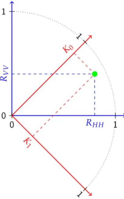
c.f., [11]. Thanks to its orthogonality, this transform restricts to a rotation and an inversion of the incident axes as shown in Figure1. The scale remains untouched, that is, the transform does not amplify or damp the original signal. Even the relative angles between the channels are equal in order to prevent additional correlations.
RHH RV V 0 1 0 1 K0 K 1 1 1
Figure 1.The orthogonal transform from reflectance (blue) to Kennaugh elements (red) in the two dimensional space of one measurement (green) according to Equation (2).
2.1.2. The Quaternion Basis
The transform given above is only applicable to two-dimensional spaces. Regarding dual-polarized acquisitions with fixed phase measurements or the up-to-date compact-hybrid mode, four channels are available in Kennaugh elements. Beyond SAR, most airborne camera or scanning systems provide a four-channel image containing Blue, Green, Red, and Infrared. For this case, an extended approach was already published in Reference [28] that formulated a four-by-four matrix with the required characteristics. For conformity reasons, an equivalent matrix is now created by the substitution of each element inC(see Equation (2)) by another complex number. Referring the coefficients to numbers, the four-by-four matrixQis created, which constitutes the Quaternion basisQ.
~ K4=Q·~R4= √1 2 " C C C −C # ·~R4= 1 2 1 1 1 1 1 −1 1 −1 1 1 −1 −1 1 −1 −1 1 ·~R4 (3)
The only difference to theAmatrix published in Reference [28] is the order and orientation of the single dimensions which is—by the way—irrelevant for its application. This matrix has already been used for the fusion of images from Sentinel-1 and Sentinel-2. The inspection of the polarimetric information content after the image fusion proofed that the polarimetric information of the input images was retained or even complemented [28].
2.1.3. The Octonion Basis
In order to serve higher-dimensional problems in the same way, the elements 1 or−1 of matrix Q(see Equation (3)) again are replaced by complex entries leading to the Octonion basis Owith eight dimensions. ~ K8=O·~R8= 1 √ 2 " Q Q Q −Q # ·~R8= 1 2 C C C C C −C C −C C C −C −C C −C −C C ·~R8 (4)
Eight channels are especially needed for the fusion of Sentinel-1 (dual-polarized) and Sentinel-2 (10 m pixel) images when both, the polarimetric and the spectral information, shall be preserved. The article cited above was titled “SAR sharpening” and thus, only cared for the polarimetric information content [28]. Due to the reduction of the dimensionality from eight to four, a minimum data loss is indisputable. Using the new Equation (4) the eight input channels again result in eight output channels, thus the information preserving transform is guaranteed.
2.1.4. The Sedenion Basis
When exploiting the complete information contained in a Sentinel-2 image, thirteen channels are involved whereas channel 8 and 8Aonly differ in their spectral and spatial resolution, that is, twelve independent channels. In combination with the four Kennaugh elements of Sentinel-1, the need for a sixteen channel transform arises which can be fulfilled by a fusion on the Sedenion basisS.
~ K16=S·~R16= 1 √ 2 " O O O −O # ·~R16 = 1 2 Q Q Q Q Q −Q Q −Q Q Q −Q −Q Q −Q −Q Q ·~R16 (5)
Thus, the Sedenion basis is able to reproduce the whole information content of a combined Sentinel-1 and Sentinel-2 image which will be of highest interest for monitoring purposes in the near future due to the high temporal sampling (at least once a week) and the easy data access at no charge. 2.1.5. Higher Order Bases
With view to coming satellite mission like EnMAP with a hyperspectral sensor on board and therewith, a much higher number of channels, the extension to high-dimensional spaces could be of interest. Due to the consistent spanning of higher-order vector spaces by simple substitution of the input elements, the extension to 32 dimensions (Equation (6)), to 64 dimensions (Equation (7)), to 128 dimensions (Equation (8)), or even more is possible without (theoretical) limitations.
~ K32=Z·~R32= 1 √ 2 " S S S −S # ·~R32 (6) ~ K64 =V·~R64= 1 √ 2 " Z Z Z −Z # ·~R64 (7) ~ K128=H·~R128= 1 √ 2 " V V V −V # ·~R128 (8)
In the case of a minimally lower number of distinct input channels, the respective channel can simply be set to zero leading to a equally lower number of independent output elements as already stated in the context of the Kennaugh decomposition in Reference [11]. Thus, a very flexible, but completely consistent feature space for the fusion of arbitrary reflectance and even further rasterized GIS layers is given. At this point we can answer the first research question: multi-layer data sets can easily be transformed to Kennaugh-like elements using extensions of the complex plane defined in (2) to so-called hypercomplex bases.
2.2. Multi-Source Image Fusion
The following section summarizes the strategies for data fusion on the hypercomplex bases introduced above subdivided to the typically available data sets.
2.2.1. Polarimetric Fusion
The fusion of multi-polarized data sets to pseudo-polarimetric images was realized by the completion of redundant Kennaugh elements in one acquisition by the distinct Kennaugh elements of another acquisition [28]. This additive approach was successfully applied to data acquired in the pursuit-monostatic phase of den TanDEM-X mission for the generation of pseudo-quad-polarized images from two dual-polarized acquisitions [63].
~
Kfused=~Kdual-co-pol+~Kdual-cross-pol (9)
This symbolic formulation can be further refined by introducing the individual spatial resolution [28], that is, the look factor as weight of the input channels. For clarity reasons, only the equally weighted, and therewith the orthogonal case, was considered.
2.2.2. SAR Sharpening
Multi-polarized images generally suffer from a reduced spatial coverage and resolution. To avoid the reduced spatial sampling, an intensity image~Kpolof higher spatial resolution can be introduced in
the same way pan-sharpening is done on optical imagery. In the simplest case, the total intensity of the multi-polarized image~Kpolis completely replaced.
~ Ksharpenend = 0 K1 K2 K3 pol + K0 0 0 0 int = 0 0 0 0 0 1 0 0 0 0 1 0 0 0 0 1 ·~Kpol+ 1 0 0 0 0 0 0 0 0 0 0 0 0 0 0 0 ·~Kint (10)
Though exemplarily shown by a four-channel image, it can be transferred to any polarimetric combination without any limitation. The intensity layer is not restricted to SAR intensities, but can even be given by the panchromatic channel of an airborne camera system as proven in Reference [28]. 2.2.3. Spectral Fusion
The fusion of multi-spectral data requires the primary transform from reflectance values to Kennaugh-like elements as already presented in Reference [28]. If the channels are drawn from different sensors~Raand~Rb, the matrix multiplication can be divided in two additive parts.
~ Kfused= 1 √ 2 " C 0 C 0 # " ~Ra ~Rb # + √1 2 " 0 C 0 −C # " ~Ra ~Rb # = √1 2 " C C # ~ Ra+√1 2 " C −C # ~ Rb (11)
Due to simplicity, the approach is demonstrated in four-dimensional space, but without any limitation of the generality.
2.2.4. SAR-Optical Fusion
The problem occurring when fusing multi-polarized SAR and multi-spectral optical data lies in the combination of already transformed Kennaugh elements~KSARin the case of SAR and reflectance values
~
ROPTin the case of optical images. We simply circumvented this problem by replacing√C2·~Ra=~KSAR
in Equation (11) and got following equation. ~ KSAR&OPT= " ~ KSAR ~ KSAR # +√1 2 " C −C # ·~ROPT= " ~ KSAR ~ KSAR # + " ~ KOPT ~ KOPT # (12) The consistent derivation explained in Section2still guarantees an orthogonal transform of the original features space even if the transform is split into two independent steps as described in Equation (12).
2.2.5. Image Fusion with Arbitrary Layers
The propertyreflectancein Optics orintensitywith respect to SAR essentially denoted that this input layer was subject to a ratio scale, that is, there was a well-defined origin and the ratio between entries was playing the key role. It further implied that the data range was restricted to positive values. Therewith, any layer in ratio scale could be transformed—in combination with others—to the Kennaugh-space. If the ratio scale was not assured and only a cardinal scale can be accepted because of negative entries (e.g.) the inclusion of this layer has to be done in a scaled version of the Kennaugh-like elements which will be presented in the following Section2.4. The summary of this section answered the second research question: simple matrix multiplication allowed us to separate the calculation of Kennaugh elements from SAR and Kennaugh-like elements from Optics and to fuse the transformed elements afterwards. The information retain was guaranteed because of the orthogonality of the transform. The fusion was performed in an additive way which considers the signal-to-noise ratio. Furthermore, the Kennaugh elements from SAR were well-known for their robustness towards noise. 2.3. Multi-Temporal Image Fusion
The multi-source image fusion mentioned above was designed to fuse images of different sensors, but taken at (approximately) the same time. This section introduces a methodology how
to generate multi-temporal Kennaugh-like matrices from multi-source Kennaugh-like elements by a matrix multiplication from the right with one of the orthogonal matrices given above. Instead of multi-temporal and multi-spectral dimensions, multi-row and multi-column measurements could be processed in the same way in order to represent spatial characteristics, for example, as supplement or even substitute to spatial convolutions in machine learning algorithms.
2.3.1. Change Detection
The simplest case is the comparison of two images, in general a pre-event image at timet1 and a post-event image at timet2. The multi-temporal Kennaugh matrix was calculated by a right multiplication with the basis of the complex planeCwhich results in the sum and the difference of the two input images.
K4×2= n Q·h ~Rt2 ~Rt1 io·C=h ~Kt2 K~t1 i·C= √1 2· " ~ Kt2+~Kt1 ~ Kt2−~Kt1 #T (13) This conformed to the normalized intensity difference in Reference [11] and the additive formulation of the differential Kennaugh elements envisaged in Reference [64]. As the first element of Kreferred to an intensity measure, the requirements for a subsequent normalization were fulfilled. The quaternion basisQfor the multi-source fusion was chosen without limiting the generality: the number of dimensions in temporal and spectral direction were completely independent.
2.3.2. Gradients and Curvature
Considering more than two images, for example, four datest1,t2,t3, andt4, more descriptors than sum and difference could be evaluated. The temporal combination then was realized by the quaternion basisQlikewise resulting in a four by four matrix of "differential" Kennaugh-like elements.
K4×4= n Q·h ~Rt4 ~Rt3 ~Rt2 ~Rt1 io·Q= 1 2· ~ Kt4+~Kt3+~Kt2+~Kt1 ~ Kt4−~Kt3+~Kt2−~Kt1 ~ Kt4+~Kt3−~Kt2−~Kt1 ~ Kt4−~Kt3−~Kt2+~Kt1 T (14)
The matrixK4×4could be interpreted as follows: the first column refers to the sum of all Kennaugh
elements, that is, to a most stable mean image or a low pass filter. The second column highlighted high frequency gradients or a high pass filter. The third column calculated the mean temporal gradient or a band pass filter. The fourth column produced the temporal curvature. All descriptors were given in critical sampling, but representing the whole information contained in the source products due to the orthogonality of the transformation matrix.
2.3.3. General Time Series Analysis
The Sentinel-1 mission with its repeat pass acquisitions every six days delivers sixteen images for a quarter of a year. In this case, the temporal fusion could simply be replaced by the Sedenion basisS without limitation of the generality.
K4×16= n
Q·h ~Rt16 . . . ~Rt1 io·S=h ~Kt16 . . . ~Kt1 i·S (15) With respect to longer time spans, hypercomplex bases of higher order were also possible, for example, theZmatrix for half a year or theVmatrix for a whole year, see Section2.1.5. The inclusion of further image layers would require the substitution ofQat the left of Equation (15) and therefore, led to an increase of the number of rows, that is, longer~Kvectors. In any case, the concept guaranteed that the first element always consists of an intensity measure that could be used for the normalization of all other
elements. To conclude, we could affirm the third research question: it was possible to introduce the time as new dimension in the same way that multi-source images were combined. Thus, the consistency of the framework was guaranteed. The identical procedure allows equally the inclusion of spatial features like multi-row and multi-column image chips for a robust description of spatial patterns.
2.4. Data Scaling Approach
This section treats the possible scaling variants of the defined elements which can be linear, logarithmic, or even normalized to a closed range with respect to the application. The origin of the elements—vectors from multi-source or matrices from multi-temporal data—is completely irrelevant. 2.4.1. Linear Scale
All image data from optical remote sensing satellites were delivered in reflectance values, mostly multiplied by a calibration factor in order to guarantee integer value. SAR data in contrast was given as real- and imaginary part in single look slant range products or amplitude data in the case of ground range or geocoded products. The conversion from the delivered scaling to intensity values could be found in the respective product specifications. The data range of linearly scaled reflectance data is given byRlinear ∈ [0,∞]whereas the mode of the exponential distribution could be found slightly
above zero. The adequate storing in digital numbers therefore was quite difficult which resulted in a high radiometric sampling of usually at least 16 bit nowadays.
2.4.2. Hyperbolic Tangent Normalized Scale
In order to reduce the bit depth without noteworthy loss of information a normalization approach was introduced in Reference [11]. The core of his hyperbolic tangent (TANH) normalization was a division of all Kennaugh elements exceptK0by the total reflectance contained inK0—the first element
of the vector or the first element of the main diagonal, respectively,—and the reduction ofK0to a
reference intensityIRe f similar to differential Kennaugh elements [13] where the pre-event intensity
served as reference for the post-event intensity. ~k=h K0−IRe f K0+IRe f K1 K0 · · · Km K0 iT (16) The resulting normalized elements shared a closed data range of~k∈[−1,+1]which simplified not only the interpretation based on Support Vector Machines (e.g.), but also the conversion to digital numbers. The standard sampling of 16 bit enables a data range of±48 dB with a maximum radiometric sampling of 0.0003 dB. The reduction to 8 bit still covered a range of±24 dB with a maximum radiometric sampling of still 0.07 dB. The range where the radiometric sampling was better than 1 dB is given by±41.7 dB and±17.5 dB, respectively. Thus, the loss of information should be negligible in comparison to a conversion of the linearly scaled variables. The possible reduction of the radiometric sampling to only a few bins enabled new classification approaches like the histogram classification [26].
2.4.3. Logarithmic Scale
The reason why TANH normalized values could be expressed in decibel, thus in logarithmic scale was pointed out in Reference [11]. It could be shown that the area hyperbolic tangent of the normalized elements gave the variables in logarithmic scale which differed from the unit decibel only by a constant factor which was the same for all normalized Kennaugh-like elements includingK0.
~kdB=atanh~kdB·20dB
ln 10 =atanh
The logarithmic scale was suitable when layers in cardinal scale should be included on the one hand, see Section2.2.5. On the other hand, it resulted in layers with more or less a normal distribution which was required by many parameter-based classification approaches like the maximum likelihood classification. Regarding data compression, the logarithmic scaling was superior to the linear scaling because of the variable sampling rate (high around zero and lower towards infinity), but inferior to the normalized scaling because of its open data range~kdB ∈[−∞,+∞].
2.5. Evaluation Approach
The evaluation of data fusion approaches was not a trivial task. Most scientists conducted a whole classification for each data set as well as for the fused one separately and compared the classification results. The improvement was expected to show up in a lower number of misclassifications using the fused data set. This was truly an adequate approach for a predefined combination of data set, classification task, and algorithm. As we were aiming at a universal approach for the data preparation, it was neither reasonable to focus on one application case nor possible to cover all possible applications. Therefore, we decided in favour of following validation strategy composed of traditional and novel methods.
2.5.1. Visual Inspection
Though very subjective, the visual inspection of imagery still was the most reliable interpretation technique with view to extremely complex or high-dimensional tasks. The high dimensionality was present in the multi-source and multi-temporal fusion. Regarding the Quaternion transform, four spectral (or polarimetric) dimensions met four temporal dimensions, which resulted in sixteen elements. The semantic subsampling to a few land cover classes was also very difficult, because the classes had to represent single temporal developments which could be highly variable [15]. Therefore, the multi-temporal fusion was validated by a visual inspection of RGB (Red-Green-Blue) compositions of the single multi-spectral elements along the temporal dimension which is provided by the single columns of the matrix. To support the conclusion drawn from visual inspection, the first five moments of the resulting distribution were calculated along the temporal and spectral dimension separately. They were normalized to a linear deviation, that is, the mean absolute deviation for the first moment, the standard deviation for the second moment, the third root of the kurtosis, and so forth.
2.5.2. Class Signatures
The multi-source image fusion resulted in a feature vector which was much easier to interpret. The signatures of different land cover classes were expected to by quite stable within the region of interest and thus could be described by the distribution of the belonging pixels in the normalized Kennaugh space. Correlations between the single Kennaugh elements which are taken into account in some parametric classifiers like the Maximum Likelihood Estimation (MLE) are of minor importance to modern classifiers like Random Forest (e.g.) or the multi-scale histogram classification [30], that is, due to the immense computing demand when evaluating multi-variable histograms with common statistical measures like mutual information. Our study will consider both: standard MLE and similarity estimation.
2.5.3. Maximum Likelihood Contingency Evaluation
One traditional method to compare class signatures with individual signatures was given within MLE. This parametric approach described the class signatures by multi-variate normal distributions defined via mean vector~µand covariance matrixς. The discriminator for each pixel vector ~ψin logarithmic scale [65] then unfolded to
Each pixel in the reference data set was attributed to the class with the maximum likelihood. After this step, a contingency matrix of the training areas—similar to the confusion matrix for classifications—was calculated. As this procedure had to be performed for varying radiometric resolutions, that is, different binnings, only the total accuracy and theκ-coefficient were reported as indicators for the quality of the class description.
2.5.4. Similarity of Signatures
As parametric approaches like the MLE always imply a certain distribution, non-parametric methods evaluating the empirically derived distributions exclusively such as the Correlation Coefficient, the Kullback-Leibler-Divergence, the Cross-Entropy, or the similarity were preferred nowadays. The similarity was designed especially for the comparison of discrete histograms from normalized remote sensing data with or without consideration of the inter-channel correlations [26]. For the case of normalized elements without noteworthy correlation, it unfolded to
1 Sp,q = m v u u t m
∏
j=1 n∑
i=1 q2i,j pi,j (19)wherendenotes the maximum number of bins andmthe number of dimensions compared, that is, Kennaugh-like elements. The root does not result directly from the derivation, but it balances the varying number of input elements when testing scenarios with varying numbers of input channels. The similarity had a closed data range ofSp,q ∈[0, 1]like any probability value. For visualization purposes
the unit decibelSp,q[dB] =10·log10Sp,q∈[−∞, 0]was preferable and will be used in Section3.
2.5.5. Intra- and Inter-Class Similarities
Using the signatures defined in Section2.5.2and the similarity measure given in Section2.5.4
intra-class and inter-class similarities were derived and compared in order to estimate the impact of the data fusion and scaling on the class separability. As the similarity could only be calculated for two signatures under study, the arithmetic mean of all possible combinations was chosen as representative value for the intra- and inter-class similarities. We expected high intra-class similarities and low inter-class similarities. In the optimal case, they do not converge until the radiometric sampling is very low, for example, binary. In addition to several diagrams that depicted the influence for each class separately, the mean gain over all classes was given in numbers. It composed of the difference between the mean intra-class and the mean inter-class similarity indicating the relative increase in class similarity. The mean similarities were calculated as arithmetic mean over all samples of the single classes. This equals the geometric mean of the incident class similarities, which means that it was very sensitive towards possible low outliers.
2.5.6. Gain of Intra- vs. Inter-Class-Similarity
In favour of a more comprehensive interpretation, the manifold results from the preceding section were rearranged and combined to a gain in similarity, that is, to which extent the mean similarity of signatures was increased or decreased. The gain was simply defined as difference between the mean logarithmic similarity of objects belonging to the same class over the mean logarithmic similarity of objects belonging to other classes. This reflected the logarithmic quotient of the respective similarities and could again be given in the unit decibel. It provided a measure equivalent to the total accuracy andκ-coefficient evaluated for the MLE comparison with mean class signatures, but derived from the similarity of individual signatures exclusively this time.
3. Results
The capability of the transforms shown in the previous section will by demonstrated in the following by selected examples. Understandably, the choice of examples was not sufficient to cover
all possible applications, but enough to provide a rough impression of the potential inherent to the novel technique.
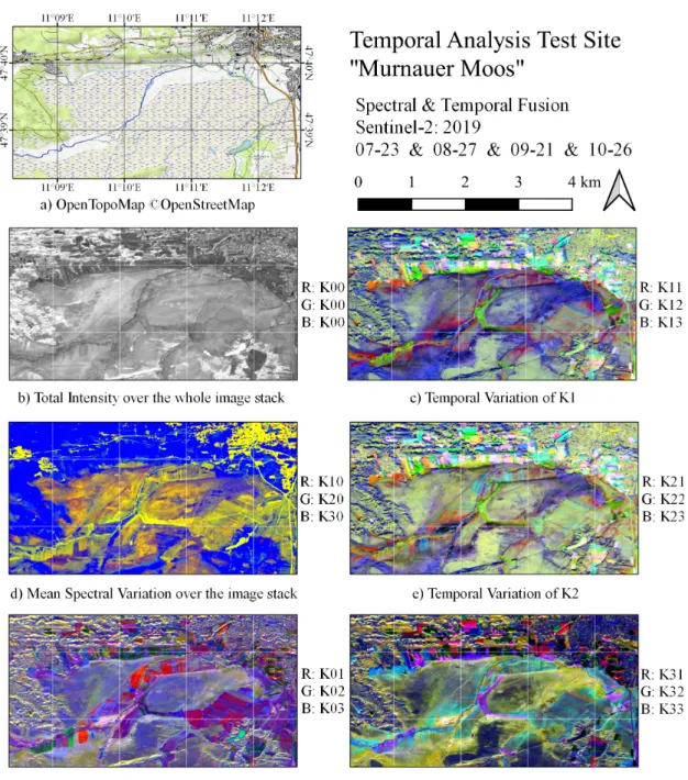
Figure 2.Sentinel-2 time series of True Colour Images (left column) and Colour Infrared Images (right column) from July to October 2019 over the “Murnauer Moos” in southern Germany. For coordinate reference, scale, and north arrow see Figure3a.
3.1. Multi-Temporal Image Fusion
The multi-temporal image fusion presented in Section2.3was applied to a data set consisting of four Sentinel-2 geocoded and atmospherically corrected L2A images over the “Murnauer Moos” near the Alps in southern Germany. The area is characterized by restored, quasi natural moor areas, agricultural land, forests, and built-up areas. Only the bottom-of-atmosphere (BOA) reflectance values contained in the 10 m-layers are considered in this example for reasons of simplicity. The almost cloud-free images were acquired on 2019-07-23, 2019-08-27, 2019-09-21, and 2019-10-26. True Colour and Colour Infrared images of the data stack were depicted in Figure2. The reflectance measures were transformed to multi-spectral Kennaugh elements according to Equation (3) and then combined to
multi-temporal elements according to Equation (14). The single rows of the resulting multi-spectral and multi-temporal Kennaugh matrix are displayed in Figure3gathered to multi-temporal RGB images, that is, each channel refers to one spectral Kennaugh element according to the indication right of the images.
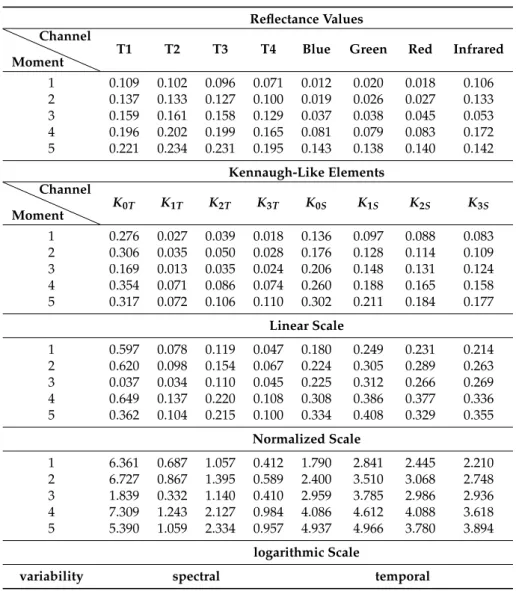
The normalized moments (e.g., the standard deviation as compared in Reference [66]) along the temporal and the spectral dimension are listed in Table1divided in the four spectral or temporal channels remaining in the respective case.
Figure 3. Multi-temporal combination of the Kennaugh elements to the four-by-four matrixK4×4
calculated of the Sentinel-2 10 m-layers imaged in July, August, September, and October 2019 over the “Murnauer Moos”, see Figure2. The depicted channels are indicated on the right side of each image. The coordinates are given in latitude and longitude on the WGS84 ellipsoid.
Table 1. Empirical central moments one to five normalized to linear deviations of the distributions adopted by the multi-spectral and multi-temporal reflectance images and Kennaugh-like elements fused on a two-dimensional Quaternion basis for the “Murnauer Moos” test site.
Reflectance Values
Moment Channel
T1 T2 T3 T4 Blue Green Red Infrared
1 0.109 0.102 0.096 0.071 0.012 0.020 0.018 0.106 2 0.137 0.133 0.127 0.100 0.019 0.026 0.027 0.133 3 0.159 0.161 0.158 0.129 0.037 0.038 0.045 0.053 4 0.196 0.202 0.199 0.165 0.081 0.079 0.083 0.172 5 0.221 0.234 0.231 0.195 0.143 0.138 0.140 0.142 Kennaugh-Like Elements Moment Channel K0T K1T K2T K3T K0S K1S K2S K3S 1 0.276 0.027 0.039 0.018 0.136 0.097 0.088 0.083 2 0.306 0.035 0.050 0.028 0.176 0.128 0.114 0.109 3 0.169 0.013 0.035 0.024 0.206 0.148 0.131 0.124 4 0.354 0.071 0.086 0.074 0.260 0.188 0.165 0.158 5 0.317 0.072 0.106 0.110 0.302 0.211 0.184 0.177 Linear Scale 1 0.597 0.078 0.119 0.047 0.180 0.249 0.231 0.214 2 0.620 0.098 0.154 0.067 0.224 0.305 0.289 0.263 3 0.037 0.034 0.110 0.045 0.225 0.312 0.266 0.269 4 0.649 0.137 0.220 0.108 0.308 0.386 0.377 0.336 5 0.362 0.104 0.215 0.100 0.334 0.408 0.329 0.355 Normalized Scale 1 6.361 0.687 1.057 0.412 1.790 2.841 2.445 2.210 2 6.727 0.867 1.395 0.589 2.400 3.510 3.068 2.748 3 1.839 0.332 1.140 0.410 2.959 3.785 2.986 2.936 4 7.309 1.243 2.127 0.984 4.086 4.612 4.088 3.618 5 5.390 1.059 2.334 0.957 4.937 4.966 3.780 3.894 logarithmic Scale
variability spectral temporal
3.2. Multi-Source Image Fusion
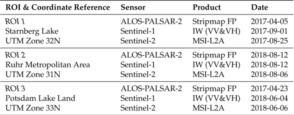
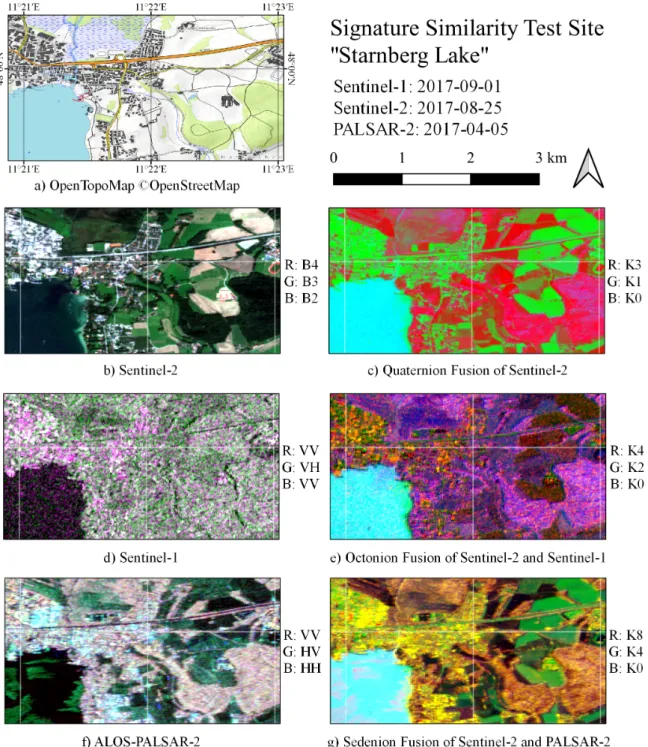
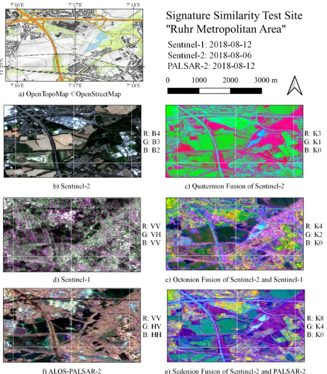
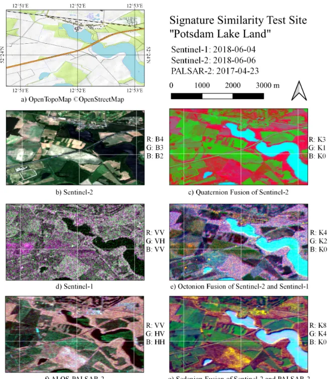
This section summarizes the results of the multi-source image fusion to one data set consisting of Sentinel-1, Sentinel-2, and ALOS-PALSAR-2 acquisitions for the three regions of interest (ROI) in Germany, namely the “Starnberg Lake” (ROI 1) in southern Germany, the “Ruhr Metropolitan Area” (ROI 2) in western Germany, and the “Potsdam Lake Land” (ROI 3) near the capital in eastern Germany. Detailed descriptions of the input data can be found in Table2. All images were projected into the earth-fixed UTM coordinate system with a uniform pixel spacing of 10 m by 10 m resulting in slightly varying look factors according to [28] which is ignored in the current study for reasons of simplicity. The following figures are all reprojected to latitude and longitude in WGS84.
The SAR data were preprocessed by the Multi-SAR System [11] exclusively available at DLR (Oberpfaffenhofen) to geocoded, calibrated, and normalized Kennaugh elements. The multi-spectral data were provided in geocoded and radiometrically calibrated BOA reflectance values and transformed into Kennaugh-like elements according to the formulas given above. The study considers two cases: a fusion on the Octonion basis including Sentinel-1 (K0,K1,K5,K8) and Sentinel-2 (B2,B3,B4,B8) and a
fusion on the Sedenion basis including ALOS-PALSAR-2 (K0−K7) and Sentinel-2 (B2−B8,B11). In all
classes: (1) Water, (2) Forest, (3) Field, (4) Meadow, and (5) Urban. The class signatures were derived from labelled segments generated in a previous study [29].
Table 2.The remote sensing data subject to the presented study.
ROI & Coordinate Reference Sensor Product Date
ROI 1 ALOS-PALSAR-2 Stripmap FP 2017-04-05
Starnberg Lake Sentinel-1 IW (VV&VH) 2017-09-01
UTM Zone 32N Sentinel-2 MSI-L2A 2017-08-25
ROI 2 ALOS-PALSAR-2 Stripmap FP 2018-08-12
Ruhr Metropolitan Area Sentinel-1 IW (VV&VH) 2018-08-12
UTM Zone 31N Sentinel-2 MSI-L2A 2018-08-06
ROI 3 ALOS-PALSAR-2 Stripmap FP 2017-04-23
Potsdam Lake Land Sentinel-1 IW (VV&VH) 2018-06-04
UTM Zone 33N Sentinel-2 MSI-L2A 2018-06-06
3.2.1. Fused Images
The visualization of Kennaugh-like elements was not an easy task because of their central distribution where the deviation from zero in both directions indicated information. The common visualization comprises three reflectance channels: Red, Green, and Blue with a non-negative exponential distribution. Therefore, the input data sets were presented in the accustomed way: True Colour Images for multi-spectral images of Sentinel-2 and Bourgeaud decomposition (i.e., the intensity channels) for SAR images of Sentinel-1 and ALOS-PALSAR-2. Out of the collection of fused Kennaugh-like elements only a selection of three elements (indicated on the right site of each image) are depicted in logarithmic scale. A subset of the images for the first region of interest can be found in Figure4. Selected subsets of the second and the third test site are illustrated in the same way in Figures5and6.
3.2.2. Signature Stability
The illustration of multi-spectral data with more than three channels was quite difficult. In optical remote sensing the four-channel information typically was divided in one true colour image (TCI) and one colour infra-red image (CIR) as illustrated in Figure2well being aware of the high redundancy. In order to generate an illustration of all eight or sixteen channels of the fused data set, histograms of three different scaling variants were computed. The linear scaling in the left column of Figures7
and8equals the standard methodology working on reflectance values (optical remote sensing) and covariance matrices (radar remote sensing), respectively. Due to the orthogonality of the transform between reflectance channels and Kennaugh-like [28] elements as well as between the covariance matrix and the Kennaugh elements [64], the statement drawn from the histograms was transferable. Elements in linear scale consist of one reflectance value (the total intensity) and several reflectance differences ranging from−∞to+∞. The second variant considered in the middle column of Figures7
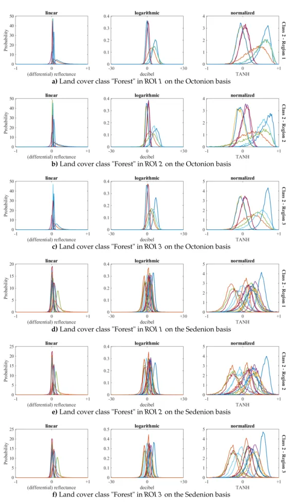
and8 was the logarithmic scaling in the unit decibel (dB) which is quite usual in radar remote sensing and electronic engineering in general. This scaling adopted a multiplicative characteristic of the input data that was supposed to be composed of intensity quotients. The typical range of decibel values—though theoretically unlimited—restricted to−30 dB to+30 dB. The normalized Kennaugh-like elements displayed in the right column of Figures7and8shared the unique property of a closed value range[−1,+1], which allowed for the most effective radiometric sampling which will be studied in the following section. In order to show the advantages of our approach two classes out of the five classes of the study which were not easy to describe with traditional methods due to their high variability were chosen for demonstration, namely “Forest” in Figure7and “Urban” in Figure8.
a)Land cover class "Forest" inROI 1on the Octonion basis
b)Land cover class "Forest" inROI 2on the Octonion basis
c)Land cover class "Forest" inROI 3on the Octonion basis
d)Land cover class "Forest" inROI 1on the Sedenion basis
e)Land cover class "Forest" inROI 2on the Sedenion basis
f)Land cover class "Forest" inROI 3on the Sedenion basis
Figure 7.The distribution of the Kennaugh-like elements on the Octonion basis fusing Sentinel-1 and Sentinel-2 (a–c) and on the Sedenion basis fusing ALOS-PALSAR-2 and Sentinel-2 (d–f) for class 2 “Forest” in linear, logarithmic, and normalized scaling per regions of interest.
a)Land cover class "Urban" inROI 1on the Octonion basis
b)Land cover class "Urban" inROI 2on the Octonion basis
c)Land cover class "Urban" inROI 3on the Octonion basis
d)Land cover class "Urban" inROI 1on the Sedenion basis
e)Land cover class "Meadow" inROI 2on the Sedenion basis
f)Land cover class "Urban" inROI 3on the Sedenion basis
Figure 8.The distribution of the Kennaugh-like elements on the Octonion basis fusing Sentinel-1 and Sentinel-2 (a–c) and on the Sedenion basis fusing ALOS-PALSAR-2 and Sentinel-2 (d–f) for class 5 “Urban” in linear, logarithmic, and normalized scaling per ROI.
3.2.3. Maximum Likelihood Contingency
The total accuracy and theκ-coefficient achieved by an MLE of the class assignment within the reference data are depicted in Figure9with respect to the ROI (line style), the input data (line colour), and the binning (right axis). The total accuracy attained 20% for only one bin which was the accuracy to be expected when five equally distributed classes were assigned randomly. Theκ-coefficient lowered to zero in this case underlining that the class assignment became purely random.
a)Total Accuracy achieved on Octonion Basis b)κ-coefficient achieved on Octonion Basis
c)Total Accuracy achieved on Sedenion Basis d)κ-coefficient achieved on Sedenion Basis
Figure 9.Total Accuracy andκ-coefficient of the contingency matrices achieved using a Maximum-Likelihood class discriminator in relation to the test site (“Starnberg Lake” solid, “Ruhr Metropolitan Area” dashed, and “Potsdam Lake Land” dot-dashed lines), the channel combination and scaling (linear reflectance, logarithmic Kennaugh-like elements, and normalized Kennaugh-like elements, see legend), and the radiometric sampling given by the number of bins.
3.2.4. Signature Similarity
The similarity of two signatures was calculated via Equation (19). In default of symmetry, the similarity measure was not commutative, that is, the similarity of class 1 to class 2 in general differed from the similarity of class 2 to class 1. Therefore, both cases were considered. For clarity reasons only the mean similarities of the respective sample class were kept in Figure10for the Octonion fusion and Figure11for the Sedenion fusion. The diagrams were split in four parts:
• upper left: the mean intra-class similarities of the individual object signatures
• upper right: the mean intra-class similarities of the mean class signatures
• lower left: the mean inter-class similarities of the individual object signatures
All similarities were provided in logarithmic scaling in the decibel unit. The searched class was indicated by the colour according to legends contained in the respective figures.
a)Mean similarities of linear elements
b)Mean similarities of logarithmic elements
c)Mean similarities of normalized elements
Figure 10.Mean intra- (upper part) and inter-class (lower part) signature similarity on the Octonion basis using (a) linear, (b) logarithmic, and (c) normalized elements evaluated with individual (left side) and mean signatures (right side) for the “Potsdam Lake Land” test site.
a)Mean similarities of linear elements
b)Mean similarities of logarithmic elements
c)Mean similarities normalized elements
Figure 11.Mean intra- (upper part) and inter-class (lower part) signature similarity on the Sedenion basis using (a) linear, (b) logarithmic, and (c) normalized elements evaluated with individual (left side) and mean signatures (right side) for the “Starnberg Lake” test site.
3.2.5. Similarity Gain
The mean gain in class similarity by comparing the intra-class to the inter-class similarities is numbered in Table3for the fusion on the Octonion basis and in Table4for the fusion on the Sedenion basis. Though, the analysis was performed separately for the three test sites, the results were quite similar. Obviously, the Sedenion fusion with its 16 channels even raised the gain in comparison to the Octonion fusion with its 8 channels. As expected the normalized Kennaugh-like elements showed the highest gain for low radiometric sampling. The gain in the logarithmic scale was remarkably variable. The linear scale was only applicable with higher radiometric sampling. In the case of the Sedenion fusion (see Table4) it only seldom exceeded the gain of normalized scaling. Regarding the Octonion fusion in Table3, the linear scaling produced higher values from 20 bins upwards. In order to provide a more detailed view to the single classes under study, selected examples of the similarity gain per class are plotted in Figure12.
Table 3. Enhancement of the mean class distinction using the Octonion basis in different scaling variants (rows) evaluated and varying number of bins (columns) for the three test sites evaluated over all samples given in decibel [dB].
ROI 1 “Starnberg Lake”
norm 15.6 16.6 15.9 17.1 15.9 15.9 16.2 12.5 8.9 11.7 7.4 4.6 3.9
log 15.0 14.7 15.9 14.0 13.6 8.7 12.5 5.7 5.3 4.3 3.8 2.3 3.9
lin 26.7 26.2 23.6 18.3 21.6 9.7 12.2 9.9 1.8 3.6 1.3 1.6 0.0
ROI 2 “Ruhr Metropolitan Area”
norm 21.2 22.3 22.3 21.7 22.4 20.3 17.9 16.2 11.9 12.9 7.4 5.6 4.7
log 20.0 20.1 19.0 17.3 16.3 12.6 12.9 7.5 7.0 6.7 5.5 3.9 4.7
lin 31.0 32.0 31.5 32.0 27.9 23.0 26.4 23.5 3.4 8.0 2.5 2.5 0.1
ROI 3 “Potsdam Lake Land”
norm 21.5 22.5 23.9 26.3 24.9 24.1 21.9 17.4 13.1 15.3 9.1 6.3 5.4
log 23.9 22.5 22.2 22.0 17.6 14.3 15.2 9.9 10.1 5.7 5.4 5.7 5.4
lin 28.4 30.4 27.2 25.2 24.6 13.7 20.6 13.7 4.2 4.9 3.2 3.5 0.2
bins 100 71 50 36 25 18 13 9 6 5 4 3 2
Table 4. Enhancement of the mean class distinction using the Sedenion basis in different scaling variants (rows) evaluated and varying number of bins (columns) for the three test sites evaluated over all samples given in decibel [dB].
ROI 1 “Starnberg Lake”
norm 34.5 34.0 36.1 37.0 35.4 33.5 30.7 25.4 21.7 13.2 19.9 7.9 15.4
log 36.4 33.7 31.5 27.2 22.8 22.2 11.5 8.5 16.4 6.5 16.1 1.3 15.4
lin 32.1 33.1 30.9 27.2 28.1 20.4 21.4 18.2 6.1 8.0 2.1 5.7 0.7
ROI 2 “Ruhr Metropolitan Area”
norm 33.4 34.6 35.4 36.6 37.1 35.7 34.6 30.3 27.8 15.2 24.8 11.4 19.0
log 35.8 34.2 33.8 31.0 27.1 28.6 13.8 13.0 20.3 7.6 20.1 2.6 19.0
lin 33.8 35.3 34.8 34.2 32.3 27.8 30.1 26.1 7.3 16.1 1.6 7.6 0.3
ROI 3 “Potsdam Lake Land”
norm 34.6 35.3 33.5 32.5 31.0 29.3 27.1 23.3 20.4 14.2 19.0 9.0 13.8
log 31.1 29.6 28.2 24.7 21.9 21.4 13.4 10.3 16.8 5.1 14.7 3.4 13.8
lin 32.6 33.4 31.7 30.0 30.4 22.3 26.0 20.0 6.2 12.2 1.5 5.4 1.0
a)"Water" samples on Octonion basis b)"Water" samples on Sedenion basis
c)"Forest" samples on Octonion basis d)"Forest" samples on Sedenion basis
e)"Field" samples on Octonion basis f)"Field" samples on Sedenion basis
g)"Meadow" samples on Octonion basis h)"Meadow" samples on Sedenion basis
i)"Urban" samples on Octonion basis j)"Urban" samples on Sedenion basis
Figure 12. Similarity gain of intra- vs. inter-class comparison for individual (left part) and mean signatures (right part) in three different scalings: normalized (solid), logarithmic (dashed), and linear (dotted) on the Octonion (left) and the Sedenion basis (right) evaluated for each class under study separately.
4. Discussion
This section interprets the results shown above and draws the conclusions concerning the application of the novel data fusion approach. In order to avoid interfering influences from varying classification methods and parameters as studied by [67], we base the whole interpretation on statistical measures and the identical set of class signatures.
4.1. Multi-Temporal Image Fusion
The benefit from the multi-temporal image fusion becomes obvious when comparing Figure3
with Figure2. The standard method based on reflectance measurements in several spectral channels suffers from the high correlation of the input channels. Therefore, mostly brightness changes are clearly visible, see Figure2. The changes in brightness are summarized in the temporal variation of the total intensityK0in Figure3f. The multi-temporal combination of the spectral properties in
Figure3d indicates that the mean spectral information content is quite low what was expected when looking at the single images in Figure2. The really characteristic changes for single land cover classes are all captured in the temporal variation of spectral Kennaugh elements. Agriculture land (e.g.) shows up in diverse colours. Especially in Figure3f,g the moor areas reveal a fine structure which was not visible at all in the standard display of Figure2. The statistical evaluation in Table1reveals three points: (1) The spectral variability in the four acquisitions (left part of the table) is equally low for reflectance values, gets variable with the transformation to linear Kennaugh-like elements, and increases significantly with the scaling of the Kennaugh-like elements. (2) The temporal variability in the right part of the table is even lower for the single spectral channels. The transformation to Kennaugh-like elements causes an increase which is again intensified when applying the typical scaling. (3) All channels show comparably high values over all five moments, that is, the underlying distributions seem to be very complex which inhibits the use the simple parametric estimators. Thus, the use of non-parametric approaches like the similarity is highly recommended. A similar validation method was already used by [68] in order to evaluate the gain by the fusion of hyperspectral and panchromatic data. Due to the complexity of the landscape, the clustering to multi-temporal class signatures is a quite difficult task and therefore, will be subject to future studies. The use of enhanced clustering methods like self-organizing (e.g.) would go far beyond the scope of this article. According to [69], the multi-temporal combination promises up to 91 % overall accuracy and 89 % for theκ-coefficient with a relatively high thematic sampling of nine land cover classes when using enhacned classification methods.
To sum up, the combination to multi-temporal Kennaugh-like elements highlights phenomena that were not apparent in the original reflectance data.
4.2. Multi-source Image Fusion
This section interprets the results of the image fusion on the Octonion and the Sedenion basis shown above. The quantitative evaluation will focus on the multi-source Kennaugh elements and take the signature stability and similarity over the classes provided in the reference data set into account. 4.2.1. Visual Inspection
The subset of the “Starnberg Lake” test site in Figure4depicts relatively smooth water and meadow areas in the optical true colour image whereas settlements appear much more heterogeneous. The SAR intensity images share the typical characteristics: smooth surfaces with respect to the wavelength are dark. The ALOS-PALSAR-2 image in Figure4f reveals some wind effect that cause a higher surface scattering in the cross-polarized channel. Regarding the meadows, Sentinel-1 shows a strong texture (Figure4d), but ALOS-PALSAR-2 relatively smooth areas (Figure 4f) due to the respective wavelength. The quite clear segments reported by the optical image are preserved and overlaid with the SAR texture when fusing both image sources on the Octonion basis in (Figure4e) or the Sedenion basis (Figure4g). Even the open water receives a certain texture that reflects the local wind situation affecting the polarimetric scattering behaviour as described above.
Figure5illustrates a subset of the “Ruhr Metropolitan Area” test site. The settlements are clearly distinguishable by their blue tone in the optical true colour image (Figure5b). In the Sentinel-1 intensity image they cannot be discriminated from the surrounding forests and meadows. The ALOS-PALSAR-2 enables the distinction between meadows that appear dark due to their smoothness with respect to the wavelength and higher objects. The appearance of settlements depends on the orientation, that
is, there are very bright spots, but also areas with a mean intensity that can hardly be discriminated from forests. The fused image unites characteristics of SAR and Optics. Settlements are mapped in yellow to red in both the Octonion (Figure5e) and the Sedenion (Figure5g) fusion according to their orientation. Agricultural land receives a slight texture that allows for a more detailed analysis of the crop. Water surfaces again appear in pale blue with a clear shape.
The most impressive example for the data fusion can be found in Figure6where a subset of the “Potsdam Lake Land” is illustrated. The clear boundaries visible in the optical image are combined with a refined SAR texture. Higher vegetation (e.g., forest) receives a fine and very diverse texture possible allowing for a more detailed analysis. Low vegetation is coloured in green tones according to the wavelength: with a higher variation in C-band (Figure6e) and a lower variation in L-band (Figure6g). Even the infrastructure is clearly mapped in the Sedenion fusion. Smooth water is exactly shaped in pale blue with only a slight pink texture in the cross-polarized channel of L-band, cf. Figure6f,e. In summary, the fused images illustrate scattering characteristics which where not visible at all in the single acquisitions. As the visual impression is often misleading [65], the three test sites are validated quantitatively in the following.
4.2.2. Mean Class Signatures
The mean class signatures of the land cover classes “Forest” and “Urban” are provided in Figures7and8for the fusion on the Octonion basis (a–c) and on the Sedenion basis (d–f), respectively. The elements in linear scale show only minor deviations from zero over all classes resulting in very slim peaks in the probability density functions (PDF), but with few very high and very low values. This effect even intensifies with an increase of input channels number from Octonion to Sedenion basis. The logarithmic scale provides diverse, but almost normally distributed elements, see middle column. The limitation to the range of [−30 dB, +30 dB] concerns only few values. Regarding typical noise levels of around−25 dB, the values exceeding the limits can be seen as noise. Some undulations become visible that indicate a higher radiometric sampling than provided by the input data. These undulations even increase in the normalized scaling, see Figure8. The closed data range and the width of the distributions allow a lower radiometric sampling with only negligible loss of information which will be studied in the following section. The signatures over the three test sites appear quite similar. The fusion on Octonion basis provides more distinct histograms than the Sedenion fusion which can be referred to the different input data, see Section3.
4.2.3. Maximum Likelihood Contingency
The total accuracy andκ-coefficient of the contingency matrix derived from a MLE class assignment proofs the advantage of the presented methodology. For a high radiometric sampling, the three methods deliver identical results. But as soon as the radiometric sampling is reduced to less than 10,000 bins, the class assignment based on reflectance values becomes more or less random (blue lines in Figure9). The logarithmic Kennaugh-like elements deliver stable results even for a radiometric sampling with only 50 bins in the Octonion case (cf. Figure9a,b) and even 25 in the Sedenion case (Figure9c,d). Regarding the normalized scaling, the accuracy of the class assignment is still clearly over 80% both in the total accuracy and theκ-coefficient for 3 bit sampling with 8 bins. For lower sampling rates, the location of the bins seems to play a key role because the neighbouring entries vary by 50% and more. A binary image (1 bit) still provides a class distinction with a total accuracy of 30% to 40% and aκ-coefficient of 20% in some ROIs. This high variability for low sampling rates is confirmed by the signature similarity analysis in the following. With respect to the fourth research question we have to admit that Kennaugh-like elements seem to provide the same accuracy in the class assignment as traditional methods as long as the bit depth is sufficient, that is, 16 bit at least. With reduced bit depths, the novel descriptor surpasses reflectance values by far.
Due to the high diversity and possibility of data combinations different methods for individual data sets and varying accuracy parameters are reported in the literature. A combination of Sentinel-1