Dynamic pricing with reference price effects

(1)

c

(2)

DYNAMIC PRICING WITH REFERENCE PRICE EFFECTS

BY ZHENYU HU

DISSERTATION

Submitted in partial fulfillment of the requirements for the degree of Doctor of Philosophy in Industrial Engineering

in the Graduate College of the

University of Illinois at Urbana-Champaign, 2015

Urbana, Illinois Doctoral Committee:

Associate Professor Xin Chen, Chair Assistant Professor Alex Olshevsky Associate Professor Nicholas Petruzzi Associate Professor Qiong Wang

(3)

Abstract

This dissertation mainly focuses on the models and the corresponding dy-namic pricing problems that incorporate reference price effects, a concept developed in economics and marketing literature that try to capture the de-pendency of consumers purchasing behavior on past prices.

Conceptually, reference price is a price expectation consumers develop from their observations of historical prices. Since it can not be physically ob-served, various models have been proposed to operationalize its formation. We empirically compare some of the models in the literature and extend the literature by proposing a new reference price model. In addition, we present analysis on the dynamic pricing problems under these models assuming con-sumers are loss/gain neutral or loss-averse. We find that constant pricing strategies are a robust solution to the problem regardless of which reference price models one may choose.

Empirical evidences, however, indicate that loss/gain neutral or loss-averse behavior may not be a universal phenomenon. We analyze the dynamic pricing problem when consumers exhibit gain-seeking behavior. In sharp contrast to the loss-averse case, even myopic pricing strategies can result in complicated cyclic price paths. We show for a special case that a cyclic skimming pricing strategy is optimal and provide conditions to guarantee the optimality of high-low pricing strategies.

With the understanding of the qualitative behavior of the optimal pricing strategies under various settings, we develop efficient algorithms to compute the optimal prices in both loss-averse and gain-seeking case. We demon-strate the efficiency and robustness of our algorithms by applying them to a practical problem with real data.

Finally, we extend the above considered single-product setting to multi-product setting and analyze the corresponding dynamic pricing problems.

(4)

(5)

Acknowledgments

First and foremost, I would like to express my deepest gratitude to my ad-visor Prof. Xin Chen. As a student, the financial support and tremendous guidance I received from Prof. Chen is what make this thesis and the com-pletion of my study possible. His quick and sharp observations have always been a source of ideas and breakthroughs. His patience, on the other hand, enables me to step out of a specific problem and to explore the related ar-eas in order to have a big picture and better understanding of the problem at hand. As a researcher, I believe the invaluable experiences of working so closely with Prof. Chen for the past four years has a profound and far-reaching influence on my future career. I get to know how a research idea is brought up and developed; I become to recognize the importance in an intuitive understanding of a certain result and I learn to keep my interests wide and open. I am eternally grateful for all the time and effort he has put in over the years to guide and teach me how to do research and how to enjoy research.

I would like to thank my thesis committee members Prof. Alex Olshevsky, Prof. Nicholas Petruzzi and Prof. Qiong Wang for their time, efforts and valuable suggestions. I would also like to thank Prof. Peng Hu for the discussions and his contributions to Chapter 3 and Chapter 4, and Yuhan Zhang for his input in Chapter 2.

During my study at the University of Illinois, I am fortunate to meet and discuss with many brilliant professors across the departments. I want to thank Prof. Enlu Zhou, Prof. Qiong Wang, Prof. Angelia Nedich and many others members of the IESE faculty for all their teachings over the years. I also want to thank Prof. Daniel Liberzon at the ECE department for the discussion in switched systems and Prof. Xiaofeng Shao at the Statistic-s department for hiStatistic-s commentStatistic-s and Statistic-suggeStatistic-stionStatistic-s on the empirical Statistic-study in Chapter 3. Finally, I would like to thank Prof. Nicholas Petruzzi at the

(6)

Business Administration department for inviting me to his review team of an academic journal paper, which is a valuable experience.

I would also like to thank the staff members at the IESE, especially Holly Kizer, Barbara Bohlen, Amy Summers. Not only they have made the offices for PhD students much more pleasant places, their dedicated works also allow me to concentrate on my studies and research.

I am grateful to the countless discussions as well as the time spent with my colleagues as well as friends in my research group, including Xiangyu Gao, Shuanglong Wang, Limeng Pan and Wenbo Chen. I am also grateful to my other friends at the University of Illinois such as Kai Jin, Fei Ji, Xinyu Ma, Haoxiang Wang, Binyang Zhang, Jingnan Chen, Fan Ye, Tao Zhu, Hao Jiang, Helin Zhu and many others for making my PhD life much more enjoyable and fun.

Finally, I am indebted to my parents for their unconditional support and encouragement. I am also indebted to my girl friend Moying Li, for her care, tolerance and love.

(7)

Appendix B . . . 110 B.1 Proof of Lemma 3.1 . . . 110 B.2 Proof of Proposition 3.1 . . . 111 B.3 Proof of Proposition 3.2 . . . 112 B.4 Proof of Lemma 3.2 . . . 113 B.5 Proof of Lemma 3.3 . . . 113 B.6 Proof of Proposition 3.3 . . . 114 B.7 Proof of Proposition 3.4 . . . 116 B.8 Proof of Proposition 3.5 . . . 117 B.9 Proof of Proposition 3.6 . . . 118 Appendix C . . . 120 C.1 Proof of Proposition 4.1 . . . 120 C.2 Proof of Lemma 4.1 . . . 120 C.3 Proof of Proposition 4.2 . . . 121 C.4 Proof of Lemma 4.2 . . . 121 C.5 Proof of Proposition 4.3 . . . 121 C.6 Proof of Proposition 4.5 . . . 123 C.7 Proof of Lemma 4.3 . . . 124 C.8 Proof of Proposition 4.6 . . . 125 C.9 Proof of Proposition 4.7 . . . 126 Appendix D . . . 127 D.1 Proof of Lemma 5.1 . . . 127 D.2 Proof of Proposition 5.1 . . . 127 D.3 Proof of Proposition 5.2 . . . 131 D.4 Proof of Lemma 5.2 . . . 132 D.5 Proof of Lemma 5.3 . . . 133 D.6 Proof of Proposition 5.3 . . . 135 References . . . 136

(9)

List of Tables

2.1 Descriptive Statistics (Chicken of the Sea 6 oz) . . . 13

2.2 Exponential Smoothing Model . . . 15

2.3 Peak-End Model . . . 15

2.4 Adaptation-Rate-Based Model . . . 16

2.5 Check of Robustness (Worst Case Analysis) . . . 16

2.6 Performance Comparisons for All Brands . . . 17

3.1 Parameter Estimates and Goodness of Fit . . . 56

3.2 Performance of Cyclic Pricing Strategies . . . 61

4.1 Parameter Estimates and Profits Comparison . . . 82

4.2 Comparison of the Computational Time for retailer: Boston - Star Market . . . 85

4.3 Growth of the number of breakpoints of Gt(q) . . . 86

(10)

List of Figures

2.1 Convergence result for benchmark model . . . 20 2.2 Ratio of steady state ranges . . . 24 2.3 _E[r(t)] and sample paths of r(t) under pH and pL . . . 27 2.4 Shape of fR∗

s(r) under different ¯α . . . 30

2.5 Comparisons of r_s∗ and r∗_D . . . 31 3.1 Possible patterns of a periodic orbit . . . 42 3.2 Discontinuous map (3.6) and periodic orbits for the myopic

pricing strategies when α= 0.8 and α= 0.85 respectively . . . 44 3.3 Optimal pricing strategy when α= 0.8, η− = 0 andγ = 0.9 . . 47 3.4 Periodic orbits for the optimal pricing strategies whenα=

0.8 andα = 0.85 respectively . . . 48 3.5 Optimal pricing strategy and a periodic orbit . . . 52 3.6 Profit comparison of simple pricing strategies . . . 59 3.7 Relative profit under different parameter combinations . . . . 60 3.8 The optimal pricing strategies when α = 0 and η−/η+ _∈

{0.16,0.18,0.20,0.22,0.24,0.26} . . . 62 4.1 Illustration of r∗(q) . . . 73 4.2 Illustration of r2(q) . . . 80

4.3 Comparison of the price paths for retailer: Boston - Star

Market . . . 84 4.4 Comparison of the price paths for retailer: Chicago - Omni . 84 5.1 State space regions and a switching path . . . 98 5.2 Steady state region and reference price paths . . . 101 D.1 Illustration of the proof . . . 134

(11)

Chapter 1

Introduction

1.1

Motivations

Over the last two decades, dynamic pricing has attracted considerable at-tention from industry as well as academia. On the one hand, the scope of industries that adopt dynamic pricing strategies has widened remarkably, with examples ranging from airline, hotel industries whose use of dynamic pricing has long been a well established practice to many other industries such as retailing, manufacturing, cloud computing and energy, etc. In retail industry, for instance, new information technology has enabled the retailers to collect information about the sales and provided them the decision-support tools for analyzing the collected data. E-commerce retailers with virtually no cost in making price changes, in particular, have brought the practice of dynamic pricing strategies to a new level. It is reported that Amazon.com, a leading e-commerce retailer, can “adjust the prices of identical goods to correspond to a customer’s willingness to pay (Weiss and Mehrotra, 2001)”. On the other hand, the on-going research in academia has led the prac-tice of dynamic pricing to grow more sophisticated over the years (see, for example, Elmaghraby and Keskinocak, 2003; Chen and Simchi-Levi, 2012, for a review). Major efforts have been devoted to several issues. First, how to capture the relationship between demand and price accurately? A recent progress in this direction is the incorporation of consumers’ behavior into consideration, such as strategic or bounded rational behavior of consumers. Second, in different business contexts, different pricing optimization models need to be developed. As an example, the stream of literature that incorpo-rates network effects into the pricing optimization models strives to tackle various pricing problems associated with the emerging social networks such as Facebook. The third issue is the coordination of pricing decisions with

(12)

other operations management decisions. A bulk of existing literature has been focusing on the coordination of pricing and inventory decisions. Fi-nally, associated with various models and problems mentioned above is the computational issue. While the models with more realistic consumer behav-iors or that incorporate other operations management decisions can bring up lots of new managerial insights, these models usually lead to very complex optimal solutions. Fortunately, the development of computational optimiza-tion techniques in mathematical programming has significantly improved the efficiency in finding optimal solutions or effective heuristics.

This thesis contributes to the existing literature in dynamic pricing through an extensive analysis of the reference price models and the corresponding dy-namic pricing problems. Traditionally, it is usually assumed that the demand in a period only depends on the selling price of the current period. However, in a market with repeated purchases such as supermarkets, intertemporal changes in prices would have significant impacts on consumers’ perception of the price and in turn influence consumers’ purchasing decisions. The concept of reference price, developed in economics and marketing literature, is then used to capture such relationship between demand and past prices. It argues that consumers form price expectations and use them to judge the current selling price. That is, reference price is used as an internal anchor formed in consumers’ minds as a result of experience based on information such as prices in observed periods (Kalyanaram and Little, 1994). Consumers then make their purchasing decisions based on the relative magnitude of the ref-erence price and the selling price. Here, a purchasing instance is perceived by consumers as gains or losses based on whether the selling price is consid-ered as discounts or surcharges relative to reference prices. Naturally, gains induce consumers to buy while losses deter them from purchasing.

Chapter 2 provides an overview of the common reference price models used in the literature. We empirically compare different reference price models, present existing results in the dynamic pricing problems and extend those re-sults. We provide answers to several important and practical questions. First, can reference price help us to capture the relationship between demand and prices more accurately? Are such findings consistent over different reference price model specifications and robust to errors in estimations? Second, what are the differences among various reference price models, both in terms of empirical performance as well as managerial implications? Finally, what are

(13)

the missing elements in the current reference price models and how will such elements change the pricing strategies of the firm?

In addition to reference price effects, behavioral asymmetry is another important consideration in modeling consumers’ behavior. A common belief is that people are loss-averse (Tversky and Kahneman, 1991) and existing literature in dynamic pricing with reference price effects has been exclusively focusing on this side of asymmetry. However, the assumption of loss-aversion is not granted to hold in every pricing context. On the contrary, many evidences including our empirical studies in Chapter 2 points to the other side of asymmetry, the gain-seeking behavior. In Chapter 3, we argue that it is necessary and important for researchers as well as practitioners to realize the existence of gain-seeking behavior. We provide analytical as well as numerical results on the dynamic pricing problem that can guide the firm in choosing its pricing strategies if it faces gain-seeking demands.

In Chapter 4, we consider the computational issues in the dynamic pric-ing problems with reference price effects. On the one hand, reference price effects link all the intertemporal pricing decisions together. On the other hand, behavioral asymmetry creates non-smooth optimization problems. In order to apply reference price models in practice, where pricing decisions for thousands of products are made and coordinated with other operations management decisions, how to compute the optimal prices efficiently and ac-curately becomes a critical question. Facing with such dynamic non-smooth optimization problems, we develop a strongly polynomial time algorithm that solves the optimal prices exactly. We identify general structural properties in the problem that make such efficient algorithm possible and many of our tech-niques are potentially applicable to other dynamic non-smooth optimization problems as well. Our algorithm is shown to be very efficient when applied to a practical problem with real data.

Most of the studies on dynamic pricing problems with reference price ef-fects in the literature (including our results in previous chapters) are in a single-product setting. While dynamic pricing problems with multiple prod-ucts are inherently difficult due to curse of dimensionality, they are, never-theless, practically relevant. Firms in retail industries, where most evidences on reference price effects are found, usually manage hundreds and thousands of products. In most cases, the demands for those products are interdepen-dent through cross-price effects. Thus, it is crucial to understand whether

(14)

the results in the single-product setting can be generalized to multi-product setting or not and if the answer is no, whether there is a simple heuristic to the problem. Chapter 5 pushes our understanding to the dynamic pric-ing problems with multiple products in this regard. We derive an explicit solution to the multi-product problem and provide a confirmative answer to the question of generalizing the results in the single-product setting for the case where no behavioral asymmetry is present. When behavioral asymme-try is considered, we provide a simple heuristic and prove several desirable properties of the heuristic.

1.2

Organization of the thesis

Chapter 2 reviews and extends the existing results by comparing the empiri-cal performance as well as managerial implications of different reference price models and proposing new models to overcome the limitations in the existing models. Section 2.1 gives a review of the empirical studies on reference price models in the literature. Section 2.2 introduces the three memory-based ref-erence price models used in the literature and the demand model to be used throughout this thesis. In Section 2.3, we give an empirical comparison of the three memory-based reference price models using real data from canned tuna category. Section 2.4-2.6 present and compare the results in the dynam-ic prdynam-icing problems under the three reference prdynam-ice models. A new reference price model is proposed and analyzed in Section 2.7.

Chapter 3 examines the dynamic pricing problem when the demand is gain-seeking. The evidences in the gain-seeking behavior and the relevant literature is presented in Section 3.1. Section 3.2 briefly reminds the read-ers of the mathematical formulation of the dynamic pricing problem. The dynamics of the myopic pricing strategy is analyzed in Section 3.3 and that of the optimal pricing strategy is analyzed in Section 3.4. Section 3.5 gives an empirical study to examine the assumptions we made and numerically examines the performance of simple pricing strategies.

Chapter 4 looks into the computational issue of the dynamic pricing prob-lems with reference price effects. Section 4.2 gives the model for the finite horizon problem. A strongly polynomial time algorithm is presented for the loss-averse demands in Section 4.3. The efficiency and robustness of the

(15)

al-gorithm is examined through solving a practical industry problem in Section 4.4.

Chapter 5 considers the dynamic pricing problem with multiple products. Section 5.1 reviews the models used in the literature for the multi-product setting and Section 5.2 introduces the model we use in a continuous time framework. In Section 5.3, we analyze the dynamic pricing problem with multiple products and give an explicit solution for the loss/gain-neutral case. For the loss-averse case, we construct a heuristic and prove some of the nice properties of the heuristic with two products.

Finally, the last chapter concludes this thesis by summarizing the directions for future research.

(16)

Chapter 2

Reference Price Models: Empirical

Comparisons and Dynamic Pricing Problems

2.1

Introduction

The concept of reference price, as introduced in Chapter 1, postulates that consumers form price expectations and use them to judge the current selling price. However, reference prices cannot be physically observed and conse-quently a large amount of literature is devoted to modeling the formation of reference prices and investigating the impact of reference prices on con-sumers’ purchasing behavior. This stream of literature can be divided into two categories based on whether the study conducted is at an individual lev-el or an aggregate levlev-el. Specifically, empirical studies based on individual level can differ in terms of models, types of data and potentially implications from the studies based on aggregate level. In most studies at the individual level, a brand choice model in multi-product setting (usually a multinomial logit model) is employed. That is, consumers’ utility function is dependent on reference price and the utility will then determine purchase probability and demands. In comparison, studies at the aggregate level demand usual-ly impose a specific demand-price function form. Correspondingusual-ly, the data used at the individual level is scanner panel data which tracks the purchasing behavior of each household while the the data used at the aggregate level is simply time series data containing price and demand pairs. Although at both levels, there are abundant evidences of reference price effects, further impli-cations on the model parameters can be different at the two levels. Readers are referred to Chapter 3 for more details on the differences.

Although the focus of this thesis is not on individual level models, we give a brief discussion of the reference price models in the literature at the indi-vidual level here for completeness. Literature in this area has differed consid-erably in how reference prices are formed and many alternative models have

(17)

been proposed and compared. There are two major different perspectives in viewing the formation of reference price. One is called the memory-based

or temporal reference price, which is assumed by a majority of researchers. They argue that reference price is based on the historical prices consumers encountered during past purchasing occasions and have operationalized ref-erence price as a weighted average of past encountered prices. For example, Mayhew and Winer (1992) and Krishnamurthi et al. (1992) have simply tak-en the price tak-encountered in the last purchase occasion as the refertak-ence price. On the other hand, Lattin and Bucklin (1989) and Kalyanaram and Little (1994) use an exponentially smoothed prices which depend on consumer’s whole purchasing history (we refer to as theexponentially smoothing model). The other one is called the stimulus-based or contextual reference price. It assumes that thecurrent pricesof certain brands serve as the reference price. The underlying argument is that consumers may not have a strong memory for past prices and the information provided by current prices of the brands available in the store is most salient and convenient for consumers. For in-stance, Hardie et al. (1993) use the current price of the brand that consumers have purchased in latest occasion as the reference price while Mazumdar and Papatla (1995) average the current prices of all brands by the weight based on the loyalties to the respective brands. Briesch et al. (1997) provide com-prehensive review of the above mentioned models and empirically compare them using scanner panel data for peanut butter, liquid detergent, ground coffee and tissue. They find that in four categories the memory-based refer-ence price model performs the best. Rajendran and Tellis (1994) postulate that a combination of both memory-based and stimulus-based reference price model may be more realistic and provide empirical evidences to support their premise.

Empirical studies at the aggregate level are relatively scarce, even though most analytical analysis in the literature is based on aggregate level models due to their simplicity. As pointed out above, aggregate level models focus more on single-product settings and even if they are generalized to multi-product settings, the brand choice behavior is not modeled explicitly. As a result, the literature at the aggregate level usually assumes a memory-based reference price model. Within the context of memory-based reference price, various operationalizations have been proposed. Similar to the individual level model, Raman and Bass (2002) use the price from the previous period

(18)

as the reference price, and Greenleaf (1995) and Kopalle et al. (1996) employ the more general exponentially smoothing model. More recently, different memory-based models have been explored. Nasiry and Popescu (2011) pro-pose a reference price model based on the peak-end rule (we refer to as the

peak-end model), which suggests that consumers remember the lowest (peak) and most recent prices (end). Such a model is conceptually supported by sub-stantial research in psychology, however, “an empirical investigation of the peak-end rule in the pricing context is still lacking (Nasiry and Popescu, 2011)”. Nevertheless, they analyze the dynamic pricing problem under the peak-end model and show that a constant pricing strategy is optimal with loss-averse consumers. Interestingly, to the best of our knowledge, neither the exponentially smoothing model nor the peak-end model is implemented in practice. Instead, it is reported in Natter et al. (2007) that bauMax, an Austrian do-it-yourself retailer, implements a further generalization of the exponentially smoothing model in their decision-support system (we refer to as the adaptation-rate-based model). In their model, consumers adapt their reference prices faster to price decreases than to price increases. They argue that quicker adaptation in case of price decreases is due to the fact that retail-ers tend to aggressively advertise price reductions while price increases may well go unnoticed by consumers. Unfortunately, no empirical comparisons to the exponential smoothing model are made in their report. In addition, since bauMax uses a price grid, they can simply evaluate all different strategies in their dynamic pricing problem and no analytical characterizations of the optimal pricing strategy are provided in the report.

This chapter then serves for the following three purposes. First, we com-plement the above mentioned literature at the aggregate level by providing an empirical comparison of different memory-based reference price models. In addition, we analyze the dynamic pricing problem with the adaptation-rate-based model and compare it with the existing results in the exponential smoothing model as well as the peak-end model. Second, we restate the es-tablished results in the literature on dynamic pricing problem for the bench-mark model: the exponential smoothing model with loss-averse demands, which not only lays down some fundamental ideas that will be used in the thesis but also gives a nice comparison to later results in Chapter 3. Finally, we point out some of the limitations of currently available reference price models and we propose by following Zhang (2011) a reference price

(19)

mod-el that incorporates randomness to address these limitations. While Zhang (2011) derives an explicit solution for the dynamic pricing problem under the stochastic reference price model, we extend his results by providing an analysis of the limiting distribution of the steady state as well as a sensitivity analysis of the expected steady state.

The remainder of this chapter is organized as follows. In Section 2.2 we present the mathematical formulation of each of the memory-based reference price models discussed above as well as the aggregate level demand model. In Section 2.3, we empirically compare the performance of the exponential smoothing model, the peak-end model and the adaptation-rate-based model using the real data on the canned tuna category. Section 2.4 presents the established results in the literature on the dynamic pricing problem under the exponential smoothing model, which serves as our benchmark model. For completeness, the results in Nasiry and Popescu (2011) for dynamic pricing problem under the peak-end model is presented in Section 2.5. The dynamic pricing problem under the adaptation-rate-based model is analyzed in Sec-tion 2.6. We introduce the stochastic reference price model and analyze the corresponding dynamic pricing problem in Section 2.7. The last section sum-marizes our findings and points out directions for future research. Proofs for the results in Section 2.7 are quite lengthy and are relegated to Appendix A. We remark here that, throughout this chapter, we consider either loss/gain-neutral or loss-averse demands and readers are referred to Chapter 3 for dynamic pricing problems with gain-seeking demands.

2.2

Reference Price and Demand Models

This section introduces the three memory-based reference price models and the demand model that describes how reference price effect affects the de-mand for a firm’s product. In the following, we use rt to denote consumers’ reference price at period t and pt to denote the shelf price of the product at period t.

(20)

2.2.1

Exponential smoothing model

As introduced in Section 2.1, the exponential smoothing model is widely used by researchers at both individual (Lattin and Bucklin, 1989; Kalyanaram and Little, 1994) as well as aggregate level (Greenleaf, 1995). It assumes that the reference price in period t+ 1 is a weighted average of the reference price in periodt and the shelf price consumers observed in periodt. Mathematically, the reference price evolves according to the following recursive formula

rt+1 =αrt+ (1−α)pt, (2.1) where α ∈ [0,1] is called the memory factor, since it captures the rate at which consumers adapt to the new price information. In the extreme case, when α = 0 consumers immediately take the price they observed in the last purchase occasion as the reference price (Raman and Bass, 2002), while when α = 1 consumers never adapt to the new price information. Usually, one would restrict α < 1, because in empirical studies α = 1 would result in pathological estimation (see Section 2.3) and in the analysis of dynamic pricing problem it would result in a static price (see Section 2.4).

2.2.2

Peak-end model

The peak-end rule postulates that memory-based decisions are made accord-ing to a combination of the most extreme and most recent experiences. By adopting this rule in the pricing context, Nasiry and Popescu (2011) assume that the peak-end experiences to be the lowest and latest price respectively. Specifically, let mt denote the lowest price consumers observed up to period

t, then the reference price follows

rt+1 =βmt+ (1−β)pt, (2.2) where β ∈[0,1] measures how much consumers anchor on the lowest price. Again, in the extreme case when β = 0, reference price is simply the price observed in the previous period. Note here that

(21)

and together with (2.2), they specify the evolution of a reference price path.

2.2.3

Adaptation-rate-based model

The adaptation-rate-based model generalizes the exponential-smoothing model in that it allows different adaptation rates based on whether con-sumers experience a price reduction or price increase:

rt+1 =pt+α+max{rt−pt,0}+α−min{rt−pt,0}, (2.3) where 0 ≤ α+ ≤ α− ≤ 1 captures the rate at which consumers incorporate the new price information depending on whether they experience a price decrease or increase. To see this more clearly, we can write (2.3) explicitly as

rt+1 =

(

α+rt+ (1−α+)pt, rt ≥pt,

α−rt+ (1−α−)pt, rt ≤pt.

The assumption α+ _≤ _α− _{then implies consumers adapt to the new price}

information pt at a faster rate when there is a price decrease than when there is a price increase. In the special case when α+ ₌_α− _:=_α_{, the above}

model reduces to the exponential smoothing model introduced in (2.1).

2.2.4

Demand model

Here, we formally introduce the aggregate-level demand model that will be used throughout this thesis. Following Greenleaf (1995), Kopalle and Winer (1996), Fibich et al. (2003) and Nasiry and Popescu (2011), the demand depends on the price pand reference price r via the model

D(r, p) =        b−ap+η+(r−p), r > p, b−ap, r =p, b−ap+η−(r−p), r < p, (2.4)

where b, a >0 and η+_{, η}− _≥_{0. More concisely, we can write} D(r, p) = b−ap+η+max{r−p,0}+η−min{r−p,0}.

(22)

Here, D(p, p) = b−ap is the base demand independent of reference prices,

η+₍_r₋_p_{) or} _η−₍_r₋_p_{) is the additional demand or demand loss induced by}

the reference price effect, where r−p is usually referred to as a perceived surcharge/discount. If r < p, consumers perceive this as a loss, while if

r > p, they perceive it as a gain. Consumers or the aggregate level demands are classified as loss-averse, loss/gain neutral and gain-seeking depending on whether η+ < η−, η+ = η− or η+ > η−. The dynamic pricing problems analyzed in this chapter all focus on either the loss-averse or loss/gain neutral case. The gain-seeking case is studied in detail in Chapter 3.

The linear form of the demand function is for the purpose of simplifying the exposition. Most of the results introduced in this thesis can be gener-alized to nonlinear forms by imposing appropriate assumptions on demand. Furthermore, the linear form allows us to conveniently estimate the corre-sponding parameters from real data on historical prices and sales using linear regression (see Section 2.3).

2.3

Model Comparison

This section complements the literature by empirically comparing the three memory-based reference price models based on the data in canned tuna cat-egory. We conduct a detailed analysis using one brand in the data set and present a summary of the performances of the models for all the brands in the data set.

2.3.1

Data and method of estimation

We utilize the data set provided by Chevalier et al. (2003) of the canned tuna product category in the Bayesm Package of the R software. The data set includes volume of canned tuna sales as well as a measure of display activity, log price and log wholesale price of seven different brands over 338 weeks.

The data set is extracted and aggregated from the Dominick’s Finer Foods database maintained by the University of Chicago Booth School of Business at http://research.chicagobooth.edu/marketing/databases/

(23)

weekly store-level data of each product sold by Dominick’s Finer Foods, a large supermarket chain in the Chicago area.

Note here that if the initial reference price andα,β,α+_/α−_{in (2.1), (2.2),}

(2.3) respectively are known, then reference prices can be generated from the historical prices and the parametersb, a, η+_{, η}− _{in the demand function (2.4)}

can be estimated using ordinary least squares (OLS). However,α,β,α+_/α−

are usually unknown and need to be estimated from the data. There is no established explicit formula for computing these parameters. Here, we follow the simple approach employed by Greenleaf (1995). For the exponential smoothing model, for instance, OLS is performed repeatedly for each value ofαvarying in increments of 0.025 from 0 to 1 (excluding 1) and our estimator

ˆ

αis chosen to be the one that maximizesR2_{. We exclude}_α _{= 1 here because}

it will result in perfect collinearity problem and OLS cannot be applied. ˆβ, ˆ

α+_{and ˆ}_α− _{are computed similarly. For initial reference price, we set it to be}

the average price for convenience throughout this section.

Table 2.1 shows the descriptive statistics of the sales, prices and reference prices computed under each of the reference price models for one item in the data set called “Chicken of the Sea 6 oz”. The corresponding estimates of α,

β and α+/α− are included in the parenthesis. One interesting observation Table 2.1: Descriptive Statistics (Chicken of the Sea 6 oz)

mean median st.dev. min max unit sales 16104 6633 49633 2525 579037 retail price ($/oz) 0.80 0.82 0.09 0.29 0.92 reference price ( ˆα= 0.325) 0.80 0.81 0.07 0.48 0.91 reference price ( ˆβ= 0.3) 0.67 0.67 0.09 0.29 0.88 reference price ( ˆα+_{= 0}_._{15, ˆ}_α−_{= 0}_.₉₇₅₎ _0.64 _0.67 _0.10 _0.34 _0.88

from Table 2.1 is that reference prices generated under peak-end model and adaptation-rate-based model are much lower than that under exponential smoothing model. The underlying intuition is that under peak-end model the lowest price can be remembered indefinitely which drags the reference price low while under adaptation-rate-based model, as argued in Section 2.2, consumers adapt more quickly to low prices.

(24)

2.3.2

Comparison results

We first present the regression results for the item “Chicken of the Sea 6 oz” and discuss some of the issues in estimation and comparison. As noted by Greenleaf (1995), the linear demand model (2.4) suffers from a multi-collinearity problem. As a result, the standard errors can be huge for some parameters and the OLS estimate to η− has a wrong sign (see, for example, the second column in Table 2.2). To tackle this problem, Greenleaf (1995) uses equity estimator and ridge estimator and obtains the correct signs. Sim-ilar regularization technique is used in the case study in Chapter 4 to another data set. However, for the canned tuna category, though ridge regression can reduce the standard errors, the estimator to η− still has a wrong sign. In-stead, we look at the restricted model by imposing η− = 0 and we report the regression results for the full model specified by (2.4), the static model which ignores reference price effects (η+ =η− = 0) and the restricted model (η− = 0).

Table 2.2-2.4 summarize the regression results for the three memory-based reference price models respectively. Two observations that are consistent in all three models can be made here. First, incorporating reference price effect-s effect-significantly improveeffect-s the goodneeffect-seffect-s of fit meaeffect-sured by R2 _{across all three}

models. The exponential smoothing model improves R2 _{by 90%, the}

peak-end model by 138% and the adaptation-rate-based model by 158% respec-tively. Second, we find the demand for this item to be gain-seeking (η+ > η−) regardless of which memory-based reference price model one chooses. In ad-dition, the estimate ofη− is statistically insignificant in all three models and the more parsimonious restricted demand model performs as good as the full demand model.

Comparing across the three tables, it is clear that the adaptation-rate-based model performs the best in terms of R2 _{or adjusted} _R2 _{for both the}

full demand model and the restricted demand model. It outperforms the exponential smoothing model by 36%. However, it only outperforms the peak-end model by 8%. Thus, one needs to be cautious when directly com-paring the three models in terms ofR2 since the adaptation-rate-based model has one more degree of freedom than the exponential-smoothing model or the peak-end model. In other words, besides the demand parameters, the adaption-rate-based model has two additional parameters (α+_and _α−_{) to be}

(25)

estimated instead of one (eitherα orβ). Therefore, it is not surprising to see a better performance from the adaptation-rate-based model. Comparatively, it is interesting to see that the peak-end model, having the same degree of freedom as the exponential smoothing model, can still outperform it by 25%.

Table 2.2: Exponential Smoothing Model

ˆ

α= 0.325 Full Model Static Model Restricted Model Intercept (ˆb) 21248 257970 14160 (0.90) (12.71)** (0.61) Price (ˆa) 27521 302613 16720 (0.96) (11.99)** (0.60) Perceived discount (ˆη+₎ ₅₇₂₆₃₀ ₅₇₃₀₆₀ (14.40)** (14.38)** Perceived surcharge (ˆη−) -57630 (-1.64) R2 _0.570 _0.300 _0.567 Adjusted R2 _0.566 _0.297 _0.564

t-statistics are in parentheses.

** significant at 1%, * significant at 5%

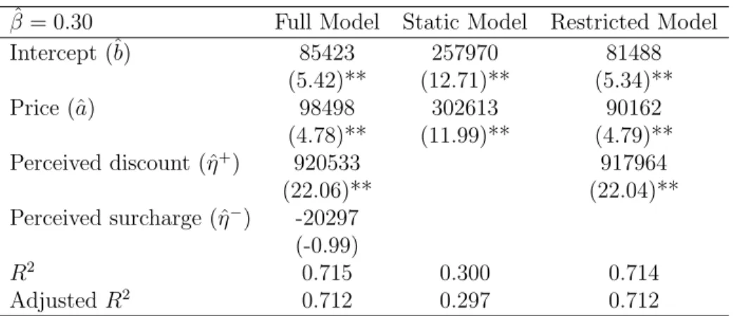
Table 2.3: Peak-End Model

ˆ

β = 0.30 Full Model Static Model Restricted Model Intercept (ˆb) 85423 257970 81488 (5.42)** (12.71)** (5.34)** Price (ˆa) 98498 302613 90162 (4.78)** (11.99)** (4.79)** Perceived discount (ˆη+₎ ₉₂₀₅₃₃ ₉₁₇₉₆₄ (22.06)** (22.04)** Perceived surcharge (ˆη−) -20297 (-0.99) R2 _0.715 _0.300 _0.714 Adjusted R2 0.712 0.297 0.712 t-statistics are in parentheses.

Actually, the issue of degree of freedom arises when reference price models are compared to the static demand model where adjustedR2 _{does not}

penal-ize on the addition of parameters α, β or α+_{, α}− _{in reference price models.}

Here, we check the robustness of our model comparisons by performing a worst case analysis. That is, for each memory-based reference price mod-el, we choose the parameters α, β or α+_{, α}− _{that minimizes} _R2 _{instead of}

(26)

Table 2.4: Adaptation-Rate-Based Model

ˆ

α+= 0.15,αˆ−= 0.975 Full Model Static Model Restricted Model Intercept (ˆb) 61669 257970 64732 (4.32)** (12.71)** (4.76)** Price (ˆa) 61997 302613 67949 (3.29)** (11.99)** (4.05)** Perceived discount (ˆη+₎ _1191648 _1190498 (26.67)** (26.68)** Perceived surcharge (ˆη−₎ ₁₀₄₉₈ (0.70) R2 _0.776 _0.300 _0.776 Adjusted R2 _0.774 _0.297 _0.774

t-statistics are in parentheses.

maximizing it. The results are summarized in Table 2.5.

Table 2.5: Check of Robustness (Worst Case Analysis)

Static Model ES PE ARB

α/β/(α+_{, α}−₎ _0.975 ₁ _{(0.975,0.975)}

R2 _0.300 _0.486 _0.502 _0.486

Adjusted R2 _0.297 _0.481 _0.498 _0.481

ES: exponential smoothing model PE: peak-end model

ARB: adaptation-rate-based model

We first observe that even under the worst case, all memory-based ref-erence price models still outperform the static demand model that ignores reference price effects. This finding is consistent with the extensive literature on reference price effects (for example Greenleaf, 1995) and further confirms the robustness of reference price effects with respect to different models and possible errors in estimations. However, under the worst case analysis, the adaptation-rate-based model no longer outperforms the peak-end model. We remark here that we have restrictedα+ ≤α−when computing the worst case for the adaptation-rate-based model. Otherwise, it will be even worse than the exponential smoothing model (with R2 _{merely 0.34). It is yet interesting}

to note that within the constraint α+ _≤ _α−_{, the worst case is attained at} α+₌_α−_{. That is, allowing consumers to adapt faster to price decreases will}

always improve the model, which supports the intuition provided in Natter et al. (2007).

(27)

memory-Table 2.6: Performance Comparisons for All Brands

Static Model ES PE ARB Star Kist 6 oz 0.190 0.359 0.449 0.360 Chicken of the Sea 6 oz 0.300 0.570 0.715 0.776 Bumble Bee Solid 6.12 oz 0.406 0.490 0.514 0.519 Bumble Bee Chunk 6.12 oz 0.259 0.640 0.664 0.650 Geisha 6 oz 0.513 0.545 0.545 0.550 ES: exponential smoothing model

PE: peak-end model

ARB: adaptation-rate-based model

based reference price models for all the brands in the data set in Table 2.6. We have excluded the two brands with large volume size: “Bumble Bee Large Cans” and “HH Chunk Lite 6.5 oz” because the estimate for a, the price sensitivity, has a wrong sign. One can see that generally, the peak-end and the adaptation-rate-based models perform better than the exponential smoothing model but the degree of improvements differ case by case. For the last three brands, the three models perform roughly the same while the peak-end model has quite an improvement over the exponential smoothing model for the first two brands. The adaptation-rate-based model, despite of the increased degree of freedom, only has significant improvement in the brand “Chicken of the Sea 6 oz”.

2.4

Dynamic Pricing under the Exponential

Smoothing Model

In this section, we present the results on the dynamic pricing problem under the benchmark model: the exponential smoothing model with loss-averse demands. This problem has been analyzed by many researchers including Kopalle et al. (1996), Fibich et al. (2003), Popescu and Wu (2007) and Asva-nunt (2007). In addition to stating existing results, we offer a new perspective in proving the steady state results in Popescu and Wu (2007). We utilize the tools from discrete dynamic system to provide a simple visualization of con-vergence and such tools enable a clearer comparison to the results to be developed in Chapter 3.

(28)

problem under the exponential smoothing model as follows: V(r0) = max pt∈[0,U] ∞ X t=0 γtΠ(rt, pt) s.t. rt+1=αrt+ (1−α)pt, t≥0, (2.5)

where Π(rt, pt) = ptD(rt, pt) is the one-period profit function and D(·,·) is defined in (2.4). Here, we have implicitly assumed that the marginal cost is 0 without loss of generality. We also assume for the remaining of this chapter that η− ≥ η+_{. Note that the assumptions} _η− _≥ _η+ _and _p _≥ _{0 allow us to}

rewrite the one-period profit as

Π(r, p) = min{Π+₍_{r, p}₎_,_Π−

(r, p)},

where

Π+(r, p) = p[b−ap+η+(r−p)], (2.6a) Π−(r, p) = p[b−ap+η−(r−p)]. (2.6b) The Bellman equation to problem (2.5) can then be written as

V(r) = max

p∈[0,U]{min{Π

+₍_{r, p}₎_,_Π−

(r, p)}+γV(αr+ (1−α)p)}, (2.7) and we usep∗(r) to denote the solution to (2.7). To solve (2.7), we introduce the following two problems:

V+(r) = max p∈[0,U]Π +₍_{r, p}_{) +}_γV+₍_αr_{+ (1}₋_α₎_p₎_, _(2.8a) V−(r) = max p∈[0,U]Π − (r, p) +γV−(αr+ (1−α)p). (2.8b) The solutions of (2.8a) and (2.8b) are denoted respectively as p+(r) and

p−(r). The following proposition gives a characterization of the solution to (2.7).

(29)

Proposition 2.1. There exists 0≤r−≤r+_≤_U _{such that} p∗(r) =        p−(r), 0≤r≤r−, r, r−≤r≤r+, p+(r), r+≤r≤U, and the optimal value function is given by

V(r) =            V−(r), 0≤r ≤r−, Π(r, r) 1−γ , r − _≤_r _≤_r+_, V+(r), r+ ≤r ≤U.

The proof to Proposition 2.1 can be found both in Popescu and Wu (2007) and Asvanunt (2007) and is omitted here. One is also referred to Section 2.6, where we prove similar results for the more general adaptation-rate-based model. We remark here that Proposition 2.1 does not rely on the linear form of the demand function and readers are referred to Popescu and Wu (2007) for the assumptions on demand and profit functions that are necessary for Proposition 2.1 to hold. With a linear form in (2.4), one can compute that r− = ₂_a₍₁₋b_γα(1₎₊₍₁−γα)₋_γ₎_η− and r+ =

b(1−γα)

2a(1−γα)+(1−γ)η+. Asvanunt (2007) also

provides explicit expressions for p−(r), p+(r) and V−(r), V+(r).

Given an initial reference price r0 and p∗(r), the sequence of reference

prices {rt} which evolves according to (2.1) is referred to as the reference

price path. A consequence of Proposition 2.1 is the following convergence result of the reference price path, which essentially says that in the long-run a constant pricing strategy is optimal.

Proposition 2.2. When r0 < r−, then {rt} is monotonically increasing and limt→∞rt = r−, when r0 > r+, then {rt} is monotonically decreasing and limt→∞rt = r+. When r− ≤ r0 ≤ r+, then rt = r0 for any t ≥ 0. Any

reference price r∈[r−, r+] is then referred to as a steady state.

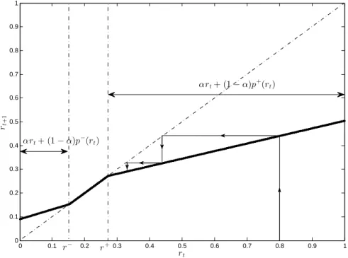
Again, the mathematical proof for Proposition 2.2 is omitted here. Instead, we give a graphical visualization of the reference price path in Figure 2.1 to illustrate both Proposition 2.1 and Proposition 2.2. In Figure 2.1, the bold

(30)

0 0.1 0.2 0.3 0.4 0.5 0.6 0.7 0.8 0.9 1 0 0.1 0.2 0.3 0.4 0.5 0.6 0.7 0.8 0.9 1 rt rt+ 1 Loss−averse Case r+ r− αrt+ (1−α)p+(rt) αrt+ (1−α)p−₍_r t)

Figure 2.1: Convergence result for benchmark model

lines represent the discrete dynamic system:

rt+1 =αrt+ (1−α)p∗(rt),

which maps rt to rt+1. The double arrowed lines specify the structures

il-lustrated in Proposition 2.1 and the arrowed lines illustrate a reference price path. Specifically, the vertical arrowed lines indicate that the trajectory e-volves from rt to rt+1 while the horizontal arrowed lines visually aid us in

thinking the function value rt+1 as an argument of the next iteration. One

can see that starting from an initial reference price r0 = 0.8> r+, the

refer-ence prices will then converge monotonically to r+.

2.5

Dynamic Pricing under the Peak-End Model

The dynamic pricing problem under the peak-end model described by (2.2) has been analyzed by Nasiry and Popescu (2011). In this section, we briefly restate their main result for completeness.

(31)

as well as the previous period price, two states are needed to describe the evolution of system. Given the initial state (m0, p0), the firm’s dynamic

pricing problem under the peak-end model is then:

V(m0, p0) = max pt∈[0,U] ∞ X t=1 γt−1Π(rt, pt) s.t. rt+1 =βmt+ (1−β)pt, t≥0, mt+1 = min{mt, pt+1}, t≥0, (2.9)

and the Bellman equation for problem (2.9) is

V(mt−1, pt−1) = max pt∈[0,U] {min{Π+₍_r t, pt),Π−(rt, pt)}+γV(min{mt−1, pt}, pt)}, rt=βmt−1+ (1−β)pt−1. (2.10) Letp∗(mt−1, pt−1) denote the optimal pricing strategy that solves (2.10) and

given the initial state (m0, p0), {p∗t} denote the optimal price path given by

p∗_t =p∗(mt−1, p∗t−1). Proposition 2.3 summarizes the main result from Nasiry

and Popescu (2011), to which one is referred for detailed analysis and proofs.

Proposition 2.3. Given any initial state(m0, p0), {p∗t} converges

monoton-ically to a steady state price, which depends only on m0.

Again, Proposition 2.3 implies that a constant pricing strategy is optimal in the long-run. However, Nasiry and Popescu (2011) note that the range of constant prices that are optimal is wider than that under the exponential smoothing model and unlike the exponential smoothing model, the optimal constant prices do not reduce to a single point when consumers are loss/gain neutral.

2.6

Dynamic Pricing under the

Adaptation-Rate-Based Model

In Section 2.3, we see that the adaptation-rate-based model achieves the best fit in one of the brand and it is actually used in practice (Natter et al., 2007). In this section, we complement the literature by analyzing the dynamic pric-ing problem under the adaptation-rate-based model.

(32)

Similar to (2.5), the firm’s dynamic pricing problem is V(r0) = max pt∈[0,U] ∞ X t=0 γtΠ(rt, pt) s.t. rt+1 =pt+α+max{rt−pt,0}+α−min{rt−pt,0}, t≥0. (2.11)

Note that we assume α+≤α−, which allows us to rewrite (2.3) as

rt+1 = min{α+rt+ (1−α+)pt, α−rt+ (1−α−)pt},

and since V(·) is continuous and monotonically increasing, the Bellman e-quation can be written as

V(r) = max

p∈[0,U]{min{Π

+₍_{r, p}_{) +}_γV₍_α+_r_{+ (1}₋_α+₎_p₎_,

Π−(r, p) + +γV(α−r+ (1−α−)p)}},

(2.12)

withp∗(r) denoting the optimal solution to (2.11). Similarly, we consider the following two problems

V+(r) = max p∈[0,U]Π +₍_{r, p}_{) +}_γV+₍_α+_r_{+ (1}₋_α+₎_p₎_, _(2.13a) V−(r) = max p∈[0,U]Π − (r, p) +γV−(α−r+ (1−α−)p), (2.13b) with the corresponding solutions denoted as p+₍_r_{) and} _p−₍_r₎

respective-ly. Proposition 2.4 characterizes the optimal pricing strategy under the adaptation-rate-based model which generalizes Proposition 2.1.

Proposition 2.4. Let r− = ₂_a₍₁₋b_γα(1−−₎₊₍₁γα−)₋_γ₎_η− and r+ =

b(1−γα+₎ 2a(1−γα+₎₊₍₁₋_γ₎_η+, then p∗(r) =        p−(r), 0≤r≤r−, r, r−≤r≤r+, p+(r), r+≤r≤U, and the optimal value function is given by

V(r) =            V−(r), 0≤r ≤r−, Π(r, r) 1−γ , r − _≤ r ≤r+, V+(r), r+ ≤r ≤U.

(33)

Proof. For 0≤s ≤1, we consider the following problem: Vs(r₀s) = max pt∈[0,U] ∞ X t=0 γtΠs(r_ts, pt) s.t. rs_t₊₁ =αsrts+ (1−αs)pt, t≥0, (2.14) where Πs(r, p) =p(b−ap+ (sη++ (1−s)η−)(r−p)) and αs =sα++ (1−

s)α−. Note that this is simply the problem with the exponential smoothing model (the memory factor isαs) and loss/gain neutral demands (the marginal reference price effect is sη++ (1−s)η−). The superscript “s” on reference price is to distinguish it from the reference prices generated in problem (2.11). In the extreme case when s = 0, Vs₍_r_{) =} _V−₍_r_{) and when} _s _{= 1,} _Vs₍_r_{) =}

V+₍_r_{). By Theorem 2 in Popescu and Wu (2007), problem (2.14) admits}

a unique steady state rs = b(1

−γαs)

2a(1−γαs)+(1−γ)(sη++(1−s)η−) and for any initial

reference pricers

0, the reference price path under the optimal pricing strategy

converges monotonically to rs. It is easy to see that r− and r+ are simply the steady states when s= 0 ands= 1 respectively.

Next, we show that Vs(r)≥V(r) for any 0≤s ≤1. We make two simple observations here. First, (sη++(1−s)η−)(r−p)≥min{η+(r−p), η−(r−p)}. Second,αsr+ (1−αs)p≥min{α+r+ (1−α+)p, α−r+ (1−α−)p}. The first observation leads to Πs₍_{r, p}₎_≥_Π(_{r, p}_{). For any initial reference price}_rs

0 =r0

and fixed price path{pt}, the second observation impliesrst ≥rtfor anyt ≥0. Since Πs₍_{r, p}_{) is increasing in} _r_{, we have Π}s₍_rs

t, pt) ≥ Πs(rt, pt) ≥ Π(rt, pt), which is true for any feasible price path {pt}. Therefore, fixing an optimal price path {p∗_t} for problem (2.11) and lettingrs

0 =r0, we then have Vs(rs₀)≥ ∞ X t=0 γtΠs(r_ts, p∗_t)≥ ∞ X t=0 γtΠ(rt, p∗t) = V(r0).

In particular, this implies V−(r)≥V(r) and V+₍_r₎_≥_V₍_r_).

When r− ≤ r ≤ r+_{, there exists 0} _≤ _s _≤ _{1, such that} _r ₌ _r

s. As rs is the steady state for problem (2.14), the pricing path{pt=rs}is optimal for problem (2.14). On the other hand, it is feasible for problem (2.11) while resulting an objective valueVs₍_r

s). ByVs(r)≥V(r),{pt=rs}is optimal for problem (2.11) as well. In other words, p∗(r) =r and V(r) =Vs(r) = Π(₁₋r,r_γ) for r−≤r≤r+.

(34)

by monotonic convergence to r− it holds p−(r) > r for 0 ≤ r ≤ r−. For any initial reference price r0 < r−, {p−(rt)} is a feasible solution to problem (2.11) and byr−≥p−(rt)> rtfor allt ≥0, it will result in an objective value

V−(r0). That is, {p−(rt)} is optimal to problem (2.11), i.e., p∗(r) = p−(r) and V(r) = V−(r) for 0≤ r ≤r−. The case for r+ _≤ _r _≤_U _{can be proven}

in a same way.

One can see from the proof of Proposition 2.4 that Proposition 2.2 can be directly generalized here. That is, the steady states for the dynam-ic prdynam-icing problem (2.11) are [r−, r+_{], where} _r− ₌ b(1−γα−)

2a(1−γα−₎₊₍₁₋_γ₎_η− and

r+ ₌ b(1−γα+₎

2a(1−γα+₎₊₍₁₋_γ₎_η+. Although the derivation of the analytical results is

similar to the exponential smoothing model, managerial implications under the adaptation-rate-based model are more in line with that of the peak-end model. Specifically, our results also imply the range of steady state prices, i.e., r+₋_r−_{, is wider than that under the exponential smoothing model. In}

the special case of loss/gain neutral demands, the optimal constant prices do not degenerate to a single price point.

0 0.1 0.2 0.3 0.4 0.5 0.6 0.7 0.8 0.9 1 0 0.1 0.2 0.3 0.4 0.5 0.6 0.7 0.8 0.9 1 α−

Ratio of the range of steady states (%)

η− = 1.5 η− = 2.0 η− = 2.5 η− = 3.0

Figure 2.2: Ratio of steady state ranges

Figure 2.2 illustrates the ratio of the steady state range under the exponen-tial smoothing model to that under the adaptation-rate-based model, where

(35)

we have fixed α=α+ _{= 0}_{, η}+ _{= 1 and} _b _{= 4}_{, a}_{= 1. One can see that when}

the loss-aversion effect is small, the adaptation-rate-based model results in relatively larger steady state ranges. Intuitively, this is due to the fact that the asymmetry in consumers’ adaptation rate dominates the asymmetry in gain/loss effects.

2.7

Stochastic Reference Price Model

In this section, we introduce a continuous time model by following Fibich et al. (2003) and along with Zhang (2011) we complement the literature by proposing a new reference price model called “stochastic reference price”. Under the stochastic reference price model, we demonstrate the behavior of reference prices and analyze the dynamic pricing problem under the assump-tion of loss/gain-neutral demands.

We first introduce the continuous time demand model as well as the con-tinuous time counterpart of exponential smoothing model (2.1). As in Fibich et al. (2003), the demand rate is still specified by (2.4) and under the as-sumption of loss/gain-neutral demands, i.e. η+ ₌ _η− ₌ _η_{, we can further}

simplify (2.4) as

D(r, p) = b−ap+η(r−p).

Given a price path {p(t)}, the continuous time counterpart of the expo-nential smoothing model is given by

(

dr = ¯α[p(t)−r(t)]dt r(0) =r0

(2.15)

where r0 is the initial reference price. We use ¯α ≥ 0 to distinguish the

parameter from the memory factor in (2.1), since here as ¯α increases, con-sumers incorporate the new price information at a faster rate while in (2.1) consumers adapt to the new price information faster as α approaches 0. Ac-cording to (2.15), with a given initial value r0 and a given price process

{p(t)}, the reference price at any given time is a fixed value for the entire consumer population.

However, there are two common features of the market that (2.15) does not capture. First, a consumer population is rarely homogeneous. For

(36)

ex-ample, brand loyal consumers and brand switchers can make different brand choice and purchase quantity decisions (Krishnamurthi et al., 1992). Thus, it is natural to postulate that each consumer should have her own perception of the prices as well. Second, other exogenous factors like advertisement ac-tivities and competitors’ prices may influence consumers’ memory processes. As argued in Section 2.1, consumers’ reference price may also be affected by contextual effects, i.e. other prices consumers observe at the time of purchase (Rajendran and Tellis, 1994).

In this section, we try to incorporate heterogeneity as well as exogenous shocks and describe the more complex behavior of consumers by using a

stochastic differential equation (SDE) (see Øksendal, 2002, for a reference on the topic of SDE) to model reference price evolution process:

dr(t) = ¯α[p(t)−r(t)]dt+σpr(t)dW(t), (2.16) where W(t) is the standard Wiener process and reference price r(t) is now a stochastic process.

Note here that for a pre-determined price path{p(t)},d_E[r(t)] =α[p(t)− E[r(t)]]dt. That is, if the firm pre-commits to a price path that is indepen-dent of the realization of randomness, then the evolution of the expected reference prices coincide with the deterministic model (2.15) used in Fibich et al. (2003). We illustrate in Figure 2.3 a sample path of (2.16) as well as _E[r(t)] under a constant pricing strategy with two price levels: the high price pH = 0.92 and the low price pL = 0.29 (the highest and lowest price in Table 2.1) respectively. In Figure 2.3, we take the initial reference price

r0 = pH+₂pL = 0.605, α = 0.5 and σ = 0.2. One can see that r(t) has a

high-er variance undhigh-er pH than under pL which reflects the square-root diffusion term in (2.16).

There are two main considerations in our choice of models. From a mod-eling perspective, we want a model that can give a good approximation to the above mentioned two features. To model consumer heterogeneity, incor-porating randomness is a common practice used in economics and marketing (see Allenby and Rossi, 1998, for instance). One possible way is to assume ¯α

to be random. However, it is easy to see that if the price is a predetermined constant, i.e., p(t) = p, for all t ≥ 0, the variance of r(t) will go to zero as

(37)

0 5 10 15 20 25 30 35 40 45 50 0 0.2 0.4 0.6 0.8 1 1.2 1.4 1.6 Time (Weeks) Reference prices r(t) under p_H r(t) under p_L E[r(t)] under p_H E[r(t)] under p L

Figure 2.3: _E[r(t)] and sample paths of r(t) under pH and pL

reference prices by employing a constant pricing strategy. While this could be plausible in some scenario, we believe, in general, variability in consumer-s’ perception of prices should persist under the common pricing strategies, such as constant, skimming or penetrating pricing strategies. On the other hand, variability in reference prices always exists (unless p(t) = 0 for all t) in (2.16). In addition, (2.16) has the nice property that the probability of

r(t) going negative is always zero. To model exogenous factors, one usually adds a random shock to represent those exogenous factors. The square-root diffusion process (2.16) has the additional merit of allowing reference price level dependent variance. It predicts that the variance of ther(t) gets smaller as r(t) itself becomes smaller. Such property is desirable in many scenarios. For instance, if competitors’ prices are a major factor affecting consumers’ memory processes, then the competitors prices would be much more attrac-tive and thus creating more variability in consumers reference prices when consumers reference prices are high rather than low.

From an analysis perspective, the square-root diffusion process (2.16) can provide analytical tractability and has found applications ranging from term-structure modeling (Cox et al., 1985) to option pricing (Heston, 1993). In our application, in particular, it enables a closed-form solution and results in a simple steady state distribution. As a result, we are able to compare analytically the expected steady state to the steady state derived from the

(38)

deterministic reference price model.

Under our stochastic reference price model, the firm’s dynamic pricing problem is V(r0) = max p(t) E Z ∞ 0 e−γtp(t)D(r(t), p(t)) dt, s.t. dr(t) = ¯α[p(t)−r(t)]dt+σpr(t)dW(t), (2.17)

where γ is the discount factor. The corresponding Hamilton-Jacobi-Bellman (HJB) equation can then be written as

γV(r) = max p {pD(r, p) + ¯α(p−r) dV(r) dr + σ2 2 r d2_V₍_r₎ dr2 }. (2.18)

Readers are referred to Miranda and Fackler (2004), for instance, for an intuitive derivation of the HJB equation (2.18). We denote p∗(r) to be the optimal solution to (2.18) andr∗(t) to be the reference price path underp∗(r) which satisfies the SDE

dr∗(t) = ¯α[p∗(r∗(t))−r∗(t)]dt+σpr∗₍_t₎_dW₍_t₎_.

Note here that by seeking a state feedback solutionp∗(r), we have implicitly assumed that the firm has the ability to measure or observe the realization of consumers’ reference price and can set a price accordingly. Similar to the problems analyzed in the previous sections, we are interested in the long-run behavior of the optimal prices as well as the resulting reference price path. Specifically, as t goes to infinity, will r∗(t) converge to a steady state? The following result gives a complete answer to this question.

Proposition 2.5. The optimal reference price pathr∗(t)converges in distri-bution to the steady state, denoted as R∗_s. The density of R∗_s is

fR∗ s(r) = (2λ/σ2₎2λµ/σ2 Γ(2λµ/σ2₎ r 2λµ/σ2₋₁ e−2rλ/σ2,

where Γ(·) is the gamma function. That is, R∗_s follows a gamma distribution with shape parameter 2λµ/σ2 _{and rate parameter} ₂_λ/σ2_{. The constants} _λ

(39)

and µ are defined by λ= ¯α2a+η−2 ¯αQ 2(a+η) , µ= ¯α ¯ αR+b 2λ(a+η),

where Q and R are given by

Q= γ 2 ¯α2(a+η) + 2a+η 2 ¯α − a+η 2 ¯α2 ∆, R= b ¯ α + σ2(a+η) ¯ α2 γ−∆ γ+ ∆ + b+ σ 2₍₂_a₊_η₎ 2 ¯α 2 γ+ ∆, and ∆ is ∆ = s γ2_{+ 2 ¯}_α2a(γ+ ¯α) +γη η+a .

Proposition 2.5 not only claims the convergence to a steady state, but also gives an explicit expression for the steady state distribution in terms of problem parameters. Our result differs from the previous literature in a sense that the steady state R∗_s is a random variable rather than a deterministic value. This confirms our motivation in modeling consumer heterogeneity: even under optimal pricing strategy, variability in consumers’ reference prices still persist.

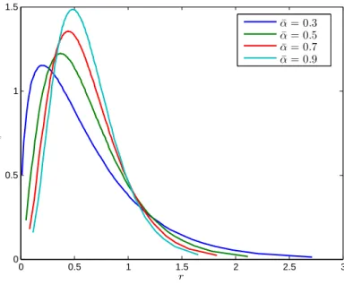
Figure 2.4 illustrates the steady state distributions under different levels of ¯α. In Figure 2.4, we have fixed a/b = 0.8, η/b = 0.5, γ = 0.01 and

σ2 _{= 0}_._{2. One can see that as ¯}_α_{grows, the spread of the distribution shrinks.}

Intuitively, this is due to the fact that as ¯αgrows, the drift term in (2.16) will have a relatively stronger effect compared to the diffusion term and result in less variance. In other words, if consumers in the population adapt to the new price information at a faster rater, then the variability in their perception of the fair prices can be reduced.

Using Proposition 2.5, we can easily compute the expected steady state reference price as well as the variance of steady state reference price. Their explicit expressions are summarized in the following proposition.

Proposition 2.6. Let ∆, µ and λ be the constants defined in Proposition 2.5. The expected steady state reference price r∗_s =_E[R∗_s] is given by

r_s∗ =µ=r∗_D+ σ 2 2a(γ+ ¯α) +γη a+η ¯ α γ 2 − ∆ 2 + 2a+η 2

(40)

0 0.5 1 1.5 2 2.5 3 0 0.5 1 1.5 r fR ∗(s r ) ¯ α= 0.3 ¯ α= 0.5 ¯ α= 0.7 ¯ α= 0.9 Figure 2.4: Shape of fR∗ s(r) under different ¯α

where r∗_D is the steady state in the deterministic problem (σ2 = 0): r∗_D = (γ+ ¯α)b

2a(γ+ ¯α) +γη. The variance of steady state reference price is given by

var(R∗_s) = µ 2λσ

2_.

We remark here thatr∗_D is exactly the steady state derived by Fibich et al. (2003) in the deterministic reference price model. Clearly, when σ = 0, our model reduces to the deterministic model in Fibich et al. (2003) and r∗_s

agrees with their solution. Whenσ >0, on the other hand, it is easy to verify that r_s∗ > r∗_D. That is, the expected steady state reference price is always higher than the steady state reference price when there is no randomness. This result is in sharp contrast with the intuition developed in some previous pricing literature. Recall in Figure 2.3 that a higher price induces a higher variability in reference price, and consequently higher variability in demands. Such variability in demands are undesirable in many settings. For example, in a joint inventory and pricing setting, by comparing the optimal price with the

riskless price (the price obtained from deterministic demands), the optimal price is always set in a way such that variability in demands is reduced

(41)

(Petruzzi and Dada, 1999). In our dynamic pricing problem, however, the firm does not need to worry about the risk of mismatch between supply and demand and demand variability will not be a concern. On the contrary, it will bring more opportunities to the firm since higher variability in reference prices will allow the firm to take advantage of the possible high reference price level. 0.1 0.2 0.3 0.4 0.5 0.6 0.7 0.8 0.9 0.59 0.6 0.61 0.62 0.63 0.64 0.65 0.66 0.67 ¯ α

Steady state reference prices

r∗ s(η/b= 0.2) r∗ D(η/b= 0.2) r∗ s(η/b= 0.5) r∗ D(η/b= 0.5) r∗ s(η/b= 0.8) r∗ D(η/b= 0.8)

Figure 2.5: Comparisons of r∗_s and r_D∗

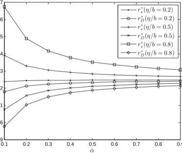
Figure 2.5 illustrates the gap betweenr_s∗ and r_D∗ under a range of values of ¯

α and different levels of η/bwith other parameters fixed at the same values in Figure 2.4. One can see that the gap decreases as ¯α increases and η/b

decreases. As ¯α grows, consumers adapt to the new price at a faster rate and in the extreme case it adjusts to the current price instantaneously. Note that this is different from the discrete time model in which case the fastest rate consumers can achieve is to adjust according to the last period price rather than the current price. Such decrease in the average gap between reference price and price reduces the (stochastic) reference price effects and consequently results in a smaller difference between r_s∗ and r_D∗. Similarly, whenη/bis small, reference price effects play a minor role and in the limiting case when η/bapproaches zero, bothr_s∗ and r∗_D get closer to thestatic price, the optimal price under the static demand model, and consequently their gap goes to zero.

(42)

More interestingly, the expected steady state reference price r_s∗ and its deterministic counterpart r∗_D can have different behaviors relative to some problem parameters. When reference price effects are significant (η/b is large), r_s∗ is decreasing in ¯α while r∗_D is increasing in ¯α. It is easy to see the monotonicity of r∗_D. Since the static price is always higher than r∗_D, as ¯α

in