Scalable Community Detection using Distributed Louvain Algorithm

University of New Orleans University of New Orleans

ScholarWorks@UNO

ScholarWorks@UNO

University of New Orleans Theses and

Dissertations Dissertations and Theses

Spring 5-23-2019

Scalable Community Detection using Distributed Louvain

Scalable Community Detection using Distributed Louvain

Algorithm

Algorithm

University of New Orleans, [email protected]

Follow this and additional works at: https://scholarworks.uno.edu/td

Part of the Computer Engineering Commons, and the Theory and Algorithms Commons

Recommended Citation Recommended Citation

Sattar, Naw Safrin, "Scalable Community Detection using Distributed Louvain Algorithm" (2019). University of New Orleans Theses and Dissertations. 2640.

https://scholarworks.uno.edu/td/2640

This Thesis is protected by copyright and/or related rights. It has been brought to you by ScholarWorks@UNO with permission from the rights-holder(s). You are free to use this Thesis in any way that is permitted by the copyright and related rights legislation that applies to your use. For other uses you need to obtain permission from the rights-holder(s) directly, unless additional rights are indicated by a Creative Commons license in the record and/or on the work itself.

This Thesis has been accepted for inclusion in University of New Orleans Theses and Dissertations by an authorized administrator of ScholarWorks@UNO. For more information, please contact [email protected].

Scalable Community Detection using Distributed Louvain Algorithm

A Thesis

Submitted to the the Graduate Faculty of the University of New Orleans

in partial fulfillment of the requirements for the degree of

Master of Science in

Computer Science HPC and Big Data Analytics

by

Naw Safrin Sattar

B.S. Bangladesh University of Engineering and Technology, 2016 May, 2019

My thesis work is wholeheartedly dedicated to my parents who tried throughout their life to provide me with the best education possible.

To my beloved husband without whose encouragement and support it was not possible to aspire for higher studies at abroad. I am thankful to my family for

keeping faith in me and providing me with the opportunity.

Last but not the least my mentor and research supervisor Dr. Shaikh Arifuzzaman for his continuous help and support from the very beginning of my

Acknowledgments

My heartiest gratitude to my advisor Dr. Shaikh Arifuzzaman for his continuous support, enthusiastic participation and invaluable guidance throughout the work. I am grateful to my spouse Md Mohiuddin Sakib who continuously motivates me and provides me with mental support to carry on with my work. I would also like to thank the members of my Thesis Committee, Dr. Mahdi Abdelguerfi, Dr. Tamjidul Hoque, and Dr. Shengru Tu. This work is partially supported by Louisiana Board of Regents RCS Grant LEQSF(2017-20)-RDA-25 and University of New Orleans ORSP Award CON000000002410. My special thanks to all of my friends and well-wishers who always have been there for any kind of support any time.

Table of Contents

Abstract . . . . . . . . . . . . . . . . . . . . . . . . . . . . . . . . . . ix

List of Figures . . . . . . . . . . . . . . . . . . . . . . . . . . . . . . . vi

List of Tables . . . . . . . . . . . . . . . . . . . . . . . . . . . . . . . vii

List of Algorithms . . . . . . . . . . . . . . . . . . . . . . . . . . . . viii Chapter 1 Introduction . . . . 1

Chapter 2 Related Works . . . . 3

Chapter 3 Background . . . . 5

3.1 Notation . . . 5

3.2 Louvain Algorithm for Community Detection . . . 6

3.2.1 Modularity Optimization Phase . . . 7

3.2.2 Community Aggregation Phase . . . 7

3.3 Computational Model . . . 8

Chapter 4 Methodology . . . . 9

4.1 Shared Memory Parallel Louvain Algorithm . . . 9

4.2 Distributed Memory Parallel Louvain Algorithm . . . 10

4.2.1 Graph Partitioning . . . 10

4.2.2 Community Detection . . . 11

4.2.2.1 Graph Initialization . . . 12

4.2.2.2 Exchange of Starting Node . . . 12

4.2.2.3 Collection of Neighbour Information . . . 13

4.2.2.4 Community Computation . . . 14

4.2.2.5 Update of Processor List for Communication . . . 16

4.2.2.6 Exchange of Updated Community . . . 18

4.2.2.7 Resolving Community Duality . . . 20

4.2.2.8 Update of Processor List for Communication in Resolving Community Duality . . . 21

TABLE OF CONTENTS

4.2.2.9 Exchange of Duality Resolved Community . . . 21

4.2.2.10 Finding Unique Communities and Computation of Modularity . . . 22

4.2.2.11 Generating Next Level Graph . . . 24

4.3 Hybrid Parallel Louvain Algorithm . . . 24

4.4 Distributed Parallel Louvain Algorithm with Load-balancing . . . 24

Chapter 5 Experimental Setup . . . . 26

5.1 Execution Environment . . . 26

5.2 Description of Datasets . . . 26

Chapter 6 Results . . . . 28

6.1 Speedup factors of shared and distributed memory algorithms . . . 28

6.2 Speedup factors of our hybrid parallel algorithm . . . 30

6.3 Speedup factors of our improved parallel algorithm DPLAL . . . 30

6.4 Runtime analysis: a breakdown of execution times . . . 32

6.5 Network size versus execution time. . . 32

6.6 METIS partitioning approaches . . . 34

6.7 Performance Analysis . . . 35

6.7.1 Comparison with Other Parallel Algorithms . . . 36

6.7.2 Comparison with Sequential Algorithm . . . 36

Chapter 7 Conclusion . . . . 38

Bibliography . . . . 40

List of Figures

4.1 Example Graph . . . 15 6.1 Speedup factors of our parallel Louvain algorithms for different

types of networks. Our hybrid algorithm strikes a balance between shared and distributed memory based algorithms. . . 29 6.2 Speedup factors of DPLAL algorithm for different types of

net-works. Larger networks scale to a larger number of processors. . . . 31 6.3 Runtime analysis of RoadNet-PA graph with DPLAL algorithm for

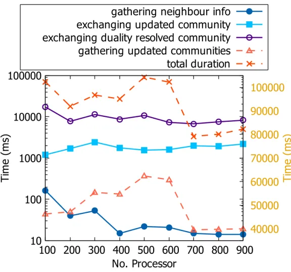
varied number of processors. We show a breakdown of execution times for different modules or functions in the algorithm. Time for gathering updated communities andtotal duration are plotted w.r.t the righty-axis. . . 33 6.4 Increase in runtime of DPLAL algorithm with an increase in the

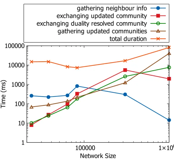
sizes of the graphs keeping the number of processors fixed. . . 34 6.5 Comparison of METIS partitioning approaches (edge-cut versus

communication volume minimization) for several networks. The edge-cut approach achieves better runtime efficiency for the above real-world networks. . . 35

List of Tables

3.1 Terminologies used in the work . . . 5

3.2 Symbols used for calculating Modularity in Equation 3.1 and Equa-tion 3.2 . . . 6

4.1 Send and Receive Count . . . 16

4.2 Community Duality . . . 20

5.1 Datasets used in our experimental evaluation. . . 27

6.1 Deviation of the number of communities for different parallel Lou-vain Algorithms from the sequential algorithm. . . 37

List of Algorithms

1 Our Parallel Louvain using MPI . . . 12

2 Gather_Neighbour_Info() . . . 17 3 Compute_Community() . . . 18 4 Update_Send_Receive_List() . . . 19 5 Exchange_Updated_Community() . . . 20 6 RCD() and EDRC() . . . 22 7 Find_Unique_Communities() . . . 23 8 Compute_ Modularity() . . . 23 9 DPLAL-Distributed Parallel Louvain Algorithm using Load-balancing 25

Abstract

Community detection (or clustering) in large-scale graph is an important prob-lem in graph mining. Communities reveal interesting characteristics of a network. Louvain is an efficient sequential algorithm but fails to scale emerging large-scale data. Developing distributed-memory parallel algorithms is challenging because of inter-process communication and load-balancing issues. In this work, we design a shared memory-based algorithm using OpenMP, which shows a 4-fold speedup but is limited to available physical cores. Our second algorithm is an MPI-based parallel algorithm that scales to a moderate number of processors. We also im-plement a hybrid algorithm combining both. Finally, we incorporate dynamic load-balancing in our final algorithm DPLAL (Distributed Parallel Louvain Al-gorithm with Load-balancing). DPLAL overcomes the performance bottleneck of the previous algorithms, shows around 12-fold speedup scaling to a larger number of processors. Overall, we present the challenges, our solutions, and the empirical performance of our algorithms for several large real-world networks.

Keywords: Community Detection; Louvain Method; Parallel Algorithms; MPI; OpenMP; Load-balancing; Graph Mining

Chapter 1

Introduction

Parallel computing plays a crucial role in processing large-scale graph data [1, 2, 3, 4]. The problem of community detection in graph data arises in many scientific domains [5], e.g., sociology, biology, online media, and transportation. Due to the advancement of data and computing technologies, graph data is growing at an enormous rate. For example, the number of links in social networks [6, 7] is grow-ing every millisecond. Processgrow-ing such graph big data requires the development of parallel algorithms [2, 8, 3, 9, 4]. Existing parallel algorithms are developed for both shared memory and distributed memory based systems. Each method has its own merits and demerits. Shared memory based systems are usually limited by the moderate number of available cores [10]. Conventional multi-core processors can exploit the advantages of shared-memory based parallel programming. The increase in physical cores is restricted by the scalability of chip sizes. Shared global address space size is also limited because of memory constraint. On the other hand, a large number of processing nodes can be used in distributed-memory systems. Although distributed memory based parallelism has the freedom of communicat-ing among processcommunicat-ing nodes through passcommunicat-ing messages, an efficient communication scheme is required to overcome communication overhead. We present a

compar-ative analysis of our shared and distributed memory based parallel Louvain al-gorithms, their merits and demerits. We have disclosed the problems arisen in communication among processes for distributed memory based parallelism [11]. We also develop a hybrid parallel Louvain algorithm using the advantage of both shared and distributed memory based approaches. The hybrid algorithm gives us the scope to balance between both shared and distributed memory settings de-pending on available resources. Load balancing is crucial in parallel computing. A straight-forward distribution with an equal number of vertices per processor might not scale well [3]. We also find that load imbalance also contribute to a higher communication overhead for distributed memory algorithms [8]. A dynamic load balancing [9, 12] approach can reduce the idle times of processors leading to in-creased speedup. Finding a suitable load balancing technique is a challenge in itself as it largely depends on the internal properties of a network and the applica-tions [13]. We present DPLAL, an efficient algorithm [14] for distributed memory setting based on a parallel load balancing scheme and graph partitioning.

Chapter 2

Related Works

There exists a rich literature of community detection algorithms [15, 16, 1, 17, 18, 19, 20, 21]. Louvain method [15] is found to be one of the most efficient sequential algorithms [18, 21]. In recent years, several works have been done for paralleling Louvain algorithm and a majority of those are shared memory based implementations. These implementations demonstrate only a moderate scalability. A Template has been proposed to parallelize the Louvain Method for Modu-larity Maximization with a shared-memory parallel algorithm [16] using OpenMP. Maximum modularity has been found by parallel reduction. They have combined communities to supervertices using parallel mergesort. They run their experimen-tal setup on two sets of LFR benchmarks of 8,000 and 10,000 vertices which is a very small number compared to dealing with large networks. Another shared-memory implementation is done using a hierarchical clustering method with adaptive par-allel thread assignment [22]. They have showed the granularity of threads could be obtained adaptively at run-time based on the information to get the maximal acceleration in the parallelization of Louvain algorithm. They have computed the gained modularity of adding a neighbor node to the community by assigning some threads in parallel. Dynamic thread assignment of OpenMP has been disabled to

let the algorithm adaptively choose the number of threads. For upto 32 cores, the speedup is not significant compared to the previous implementations PLM [17] [23] and CADS [24].

One Distributed-Memory implementation has been done in [1]. Graph parti-tioning has been done using PMETIS . They have only parallelized the first level for speedup. Each MPI process locally ignores cross partition edges, that might be an issue with accuracy. They have used three different vertex ordering strategies but none of those are effective enough considering performance. Although they get a speedup in their approach but it has been flattened for most of the graphs after scaling up to 16 - 32 processors.

One of the fastest shared memory implementations is Grappolo software pack-age [25, 26], which is able to process a network with 65.6M vertices using 20 compute cores. One of the MPI based parallel implementations [1] of Louvain method reported scaling for only 16 processors. Later, in [27] the authors could run large graphs with 1,000 processing cores for their MPI implementation but did not provide a comprehensive speedup results. Their MPI+OpenMP imple-mentation demonstrated about 7-fold speedup on 4,000 processors. But the paper uses a higher threshold in lower levels in Louvain method to terminate the level earlier and thus minimized the time contributing to their higher speedup. The work also lacks on the emphasis on graph partitioning and balancing load among the processors. This is a clear contrast with our work where we focused on load balancing issue among others. Our work achieves comparable (or better in many cases) speedups using a significantly fewer number of processors than the work in [27].

Chapter 3

Background

Notations, Definitions,and computational model used are described in this section.

3.1

Notation

The network is denoted by G(V, E), where V and E are the sets of vertices and edges, respectively. Vertices are labeled as V0, V1, . . . . , Vn−1. We use the

words node and vertex interchangeably as well as links and edges. P is the num-ber of processors used in the computation, denoted by P0, P1, . . . . , PN−1 where

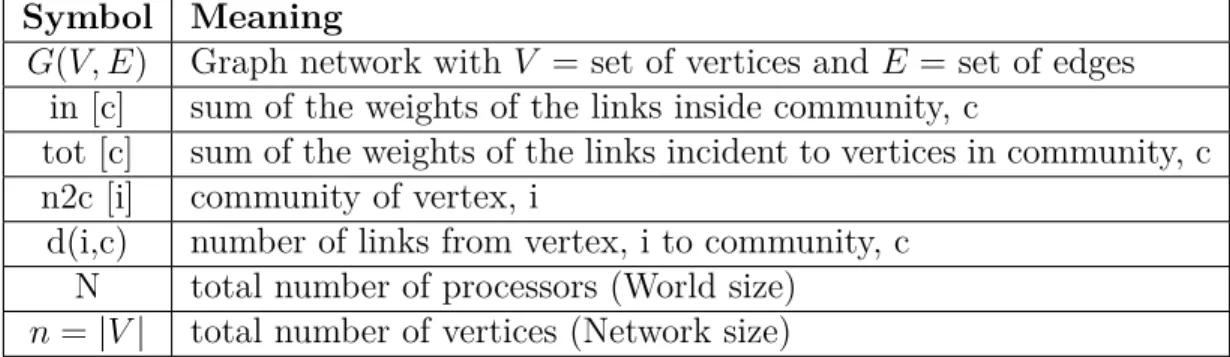
0,1,2, . . . . , N−1 refers to the rank of a processor. Terms frequently used through-out the paper, are enlisted in Table 3.1.

Table 3.1: Terminologies used in the work

Symbol Meaning

G(V, E) Graph network with V = set of vertices andE = set of edges in [c] sum of the weights of the links inside community, c

tot [c] sum of the weights of the links incident to vertices in community, c n2c [i] community of vertex, i

d(i,c) number of links from vertex, i to community, c N total number of processors (World size)

3.2

Louvain Algorithm for Community

Detec-tion

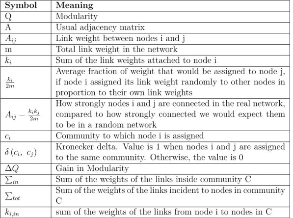
Louvain is a simple, heuristic method to extract the community structure of large networks based on modularity optimization [15]. It outperforms all other known community detection method in terms of computation time. Modularity, Q is calculated using Equation 3.1, where−1< Q <1. The meanings are described in Table 3.2. The algorithm is divided in two phases those are iteratively repeated .

Q= 1 2m X ij " Aij − kikj 2m # δ(cicj) (3.1)

Table 3.2: Symbols used for calculating Modularity in Equation 3.1 and Equa-tion 3.2

Symbol Meaning

Q Modularity

A Usual adjacency matrix

Aij Link weight between nodes i and j

m Total link weight in the network

ki Sum of the link weights attached to node i ki

2m

Average fraction of weight that would be assigned to node j, if node i assigned its link weight randomly to other nodes in proportion to their own link weights

Aij− k₂i_mkj

How strongly nodes i and j are connected in the real network, compared to how strongly connected we would expect them to be in a random network

ci Community to which node i is assigned

δ(ci, cj) Kronecker delta. Value is 1 when nodes i and j are assigned

to the same community. Otherwise, the value is 0

∆Q Gain in Modularity

P

in Sum of the weights of the links inside community C P

tot

Sum of the weights of the links incident to nodes in community C

3.2.1

Modularity Optimization Phase

For each node i the neighbours j of i are considered and the gain in modularity, ∆Q that would take place by removingi from its community and by placing it in the community of j is evaluated. ∆Q obtained by moving an isolated node i into a community C is computed using Equation 3.2.

∆Q=   P in+ki,in 2m − P tot+ki 2m !2 −   P in 2m − P tot 2m 2 − ki 2m !2  (3.2)

The symbolic meanings are given in Table 3.2. When i is removed from its communityCa similar equation is used. This continues repeatedly until no further improvement is achieved. This phase comes to an end when a local maxima of the modularity is attained.

3.2.2

Community Aggregation Phase

In this phase, a new network is formed whose nodes are the communities found during the first phase. The weights of the links between two new nodes are given by the sum of the weight of the links between nodes in the corresponding two communities. Links between nodes of the same community lead to self-loops for this community in the new network.

After completion of second phase, the first phase of the algorithm is reapplied to the resulting weighted network and iteration continues as long as positive gain in modularity is achieved.

3.3

Computational Model

At first, we develop share-memory based parallel algorithm using Open Multi-Processing (OpenMP) to eliminate the limitations of [16] with a different approach. Shared-memory based algorithms have some own limitations due to limited number of physical processing cores hindering high speedup. Therefore, we develop parallel algorithm for message passing interface (MPI) based distributed-memory parallel systems, where each processor has its own local memory. The processors do not have any shared memory, one processor cannot directly access the local memory of another processor, and the processors communicate via exchanging messages using MPI.

Chapter 4

Methodology

4.1

Shared Memory Parallel Louvain Algorithm

In shared memory based algorithms, there is a shared address space and multiple threads share this common address space. This shared address space can be used efficiently using lock and other synchronization techniques. The main hindrance behind the shared memory based systems is the limited number of processing cores. We parallelize the Louvain algorithm by distributing the computational task among multiple threads using Open Multi-Processing (OpenMP) framework. We parallelize the louvain algorithm computational task-wise in a straight-forward approach. Whenever there is a need to iterate over the full network or even the neighbors of a node, considering the large network size, the work is done by multiple threads to minimize the workload and do the computation faster.

4.2

Distributed Memory Parallel Louvain

Algo-rithm

Our aim is to compute the communities of the full network in a distributed manner. To serve the purpose, we distribute the full network among the processors in a balanced way, so that each processor can do its computation in a reasonable time and no one should wait for another. It is necessary because after each level of computation, they have to communicate with the root processor to generate the modularity of the full network. After each level of iteration, the network size decreases gradually and when the network size is considerably small, the final level is computed by a single processor which acts similar to the Louvain Sequential Algorithm.

4.2.1

Graph Partitioning

Let N be the number of processors used in the computation. The network is partitioned intoN partitions, and each processor,Pi is assigned one such partition

Gi(Vi, Ei). Processor Pi performs computation on its partition Gi. The network

data is given as input in a single disk file. While partitioning G(V, E), if the vertex-id does not start with 0, then the vertices are renumbered from 0 toni−1. The network is partitioned depending on the number of vertices of the network such that each processor gets equal number of vertices. N can vary depending on the system configuration and available resources. n is also of varied range. So, we cannot divide the vertices equally among processors when n mod N! = 0 We distribute the remaining nodes starting with processor P0 and continue up to

processor Pk(0 <= k < N), as long as the remainder lasts. Each processor has its own part of the network necessary to compute the communities in the partial

network. It is a very naive partitioning technique.

4.2.2

Community Detection

We have parallelized the sequential algorithm in such a way that each proces-sor can compute its partial network‘s community with minimized communication among the processors. The following information are needed for each processor to complete its part of computation.

• Degree of each vertex within the partition • Neighbors of each vertex

• Weight associated with each neighbor

In first phase, each processor scans through all neighboring vertices and identifies those in different processors. It then gathers the mentioned information by mes-sage passing among those processors. Then each processor locally computes the modularity of the partial network and does community detection. After computa-tion, it sends information of each vertexâĂŹs community to the processor acting as the root. The Root processor needs the value of in,tot arrays and total weight of the network to compute modularity of the full network. This full process is iterated several times as long as there is increase in modularity.

The output is stored as (node,community) for each level of iteration. It is also stored in an adjacency matrix format that is used to visualize the graph using Python‘s networkx library.

Algorithm 1 represents the pseudo-code of our approach. All the steps from Section 4.2.2.3 to 4.2.2.11 are done for each level of computation and repeated as long as we get increase in modularity value.

Algorithm 1: Our Parallel Louvain using MPI

Data: Input Graph G(V,E)

Result: (Vertex, Community) Pair 1 while increase in modularity do

2 G (V, E) is divided into p processes; 3 Each graph_i.bin contains

l n p m

vertices and corresponding edges in adjacency list format;

4 for Each processor Pi (executing in parallel) do

5 Initialize_Graph(); 6 Exchange_Starting _Node(); 7 Gather_Neighbour_Info(); 8 Compute_Community(); 9 Exchange_Updated_Community(); 10 Resolve_Community _Duality();

11 Exchange_Duality _Resolved _Community();

12 Find_Unique_Communities();

13 Compute_Modularity();

14 Generate_NextLevel_Graph();

15 if number_of_communities < i then

16 i← number_of_₂communities; 17 end

18 end 19 end

4.2.2.1 Graph Initialization

In this step, each processor Pi reads the input graph, graph_name_i.bin. If the node-id does not start with 0, then the nodes are renumbered from 0 to ni −1. Afterwards a quality object, q is created from graph, g which initializes the arrays tot, in and n2c. Line 5, in Algorithm 1 does this.

4.2.2.2 Exchange of Starting Node

In this step, each processor Pi sends own starting node-id to other processors, Pj in the communicating world.

Pimsg −−→Pj where

i, j ∈world, j= 0,1, . . . . , N −1 ^ i! =j, N =world_size

msg 3 starting_node_Pi

The number of Send and Receive operations are equal to N −1. This step is mainly required because at later phases, we use this information to find out which node belongs to which processor at other steps of our calculation. If number of processors is always a factor of network size, we could have skipped this step by numerically figuring out the starting node for each processor. This is a very rare scenario and our world size can vary depending on the system configuration and available resources. Again, network size is also of varied range. So, we cannot divide the nodes equally among processors when

n mod N! = 0, n=network_size

So, we distribute the remaining nodes starting with processorP0 and continue up

to processor Pk, as long as the remainder lasts. Here, 0<=k < N

4.2.2.3 Collection of Neighbour Information

In this step. We scan through the neighbor list of all vertices and find out the neighbors those do not belong to current processor using the information of Section 4.2.2.2. Now, we need the following information of each vertex in the neighbor list:

• weight,

• neighbor list with weights

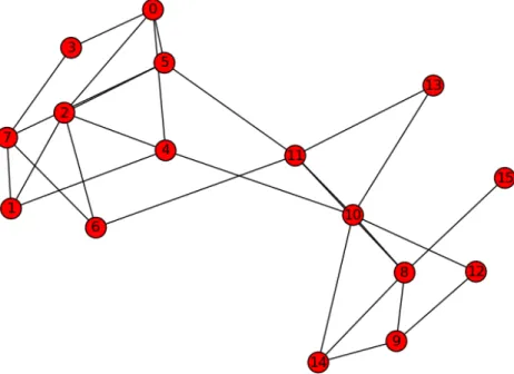
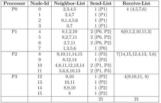
These are necessary for the calculation in section 4.2.2.4. To gather this infor-mation, we need to know beforehand, how many send and receive operations are required to communicate with other processors. To calculate the number of send-ing and receivsend-ing processors, we iterate over full neighbor list of all vertices. Here, we find out the vertices that donâĂŹt belong to current processor and identify the unique processors, we need to communicate. The number of unique processors is the size of our send-list. The number of unique vertices found from neighbor list of all the vertices, is the size of our receive-list. After receiving the desired information, we update the n2c, in and tot array entries for the aforementioned vertices and store the neighbor list with weight information for further calcula-tion. Below pseudo-code in Algorithm 2 represents this step. Table 4.1 shows an example simulation for this step. Figure 4.1 visualizes a network of 16 nodes.

4.2.2.4 Community Computation

In this step, we do the actual computation to determine community of each ver-tex. Each processor, Pi completes this step individually and locally updates the community of the vertices belonging to it.This step does not require any commu-nication among processors. A random vertex, V is chosen from the list of vertices. Then, the set of neighboring communities of that vertex is computed with the information from Section 4.2.2.3. Here, the number of links from that vertex, V to all its neighboring community is computed and stored. Next, the vertex is re-moved from its current community, Cold. Now, the modularity gain is calculated for all its neighboring communities. If the gain is maximum for community, C,

Figure 4.1: Example Graph

previous community, Cold. This, remove () and insert () operations update the in and tot arrays implicitly. As, each processor is locally updating the community, we need to keep trace if community C belongs to processorPi or not. If C belongs to processor,Pj, we simply store Vcomm =C and Vlink =dV,C wheredV,C= number of links from vertex V to Community C. These two valuesVcomm andVlink are stored separately in two arrays rem_comm and rem_dvc that we used later, described in section 4.2.2.6. This continues until all vertices from the list is covered. The pseudo-code is given in Algorithm 3

Table 4.1: Send and Receive Count

Processor Node-Id Neighbor-List Send-List Receive-List

P0 0 2,3,4,5 1 (P1) 4 (4,5,7,6) 1 2,4,7 1 (P1) 2 0,1,4,5,6 1 (P1) 3 0,7 1 (P1) P1 4 0,1,2,10 2 (P0, P2) 6(0,1,2,10,11,3) 5 0,2,7,11 2 (P0, P2) 6 2,7,11 2 (P0, P2) 7 1,3,5,6 1 (P0) P2 8 9,10,11,14,15 1 (P3) 7(14,15,12,4,13, 5,6) 9 8,12,14 1 (P3) 10 4,8,11,12,13,14 2 (P1, P3) 11 5,6,8,10,13 2 (P1, P3) P3 12 9,10 1 (P2) 4(9,10,11, 8) 13 10,11 1 (P2) 14 8,9,10 1 (P2) 15 8 1 (P2) 21 21

4.2.2.5 Update of Processor List for Communication

This is a preliminary step required for Section 4.2.2.6. After updating the com-munity of the vertices locally, we need to circulate the update globally among all processors so that each community keeps aware of the vertices in its region. Again, we need to figure out the number of sending and receiving processors before start-ing the communication. It is done in this step. We iterate over all the elements of rem_comm array and find out the processor to which that element belonged to. For each processor, we summed the total number of vertices those required update. Again, we also send to all processors of the world a message,msg containing either 0 or 1 and receiving back from all. Now, the processors those have at least one vertex that required update, are inserted into our list of sending processors and the value msg = 1. Otherwise, msg = 0. So, the receive list size is computed by summing the received value of msg.

Algorithm 2: Gather_Neighbour_Info() 1 Initialize empty array receive_list;

2 for each vertex v in g do

3 Initialize empty array send_list; 4 for each neighbor of v do

5 V_n ←neighboring node of v;

6 if V_n not in current processor then

7 Pj ← processor having Vn ; 8 if receive_list.contains() ! =V_n then 9 receive_list.push(V_n); 10 end 11 if send_list.contains() ! =P_j then 12 send_list.push(P_j); 13 end 14 end 15 end 16 for times=send_list.size() do 17 P_j ←send_list.pop(); 18 MPI_ISend(deg(v), weight(v), P_j);

19 MP_ISend (v, n2c[v], neighbors of v (node-id, weight), Pj);

20 end 21 end

22 for times= receive_list.size() do

23 MPI__Recv(deg(v‘), weight(v‘), MPI_ANY_SOURCE);

24 P_j ← status.MPI _ANY_SOURCE ;

25 MPI_Recv (v‘, n2c[v‘], neighbors of v‘ (node-id, weight), Pj);

26 Update n2c[v‘], in[v‘] and tot[v‘] locally;

27 Neighbor[v‘]. push (neighbors of v‘ (node-id, weight)); 28 end Pimsg −−→Pj where, i, j ∈world, j= 0,1, . . . . , N −1 ^ i! =j, N =world_size

Algorithm 3: Compute_Community() 1 while vertices.size()!=0 do

2 Pick random vertex, V from g ; 3 for all neighboring vertices of V do 4 Vn ←neighboring vertex of V ;

5 d_V,Vn ←number of links from vertex, V to community, V_n; 6 end

/* remove node from its current community */

7 remove (V, n2c[V],dV,V_n);

8 for all neighboring vertices of V do 9 V_n ←neighboring vertex of V ;

10 compute_gain() ;

11 if positive gain then 12 n2c[v]←n2c[V_n] ;

13 if n2c[Vn] not in current processor then

14 P_j ←processorhavingn2c[V_n]; 15 rem_comm[V_n]←n2c[V_n]; 16 rem_dvc[Vn]←dV,V_n; 17 end /* insert locally */ 18 Insert (V, n2c[V_n], d_V,Vn); 19 end 20 end 21 end msg = (1, verticesrequiringupdate >= 1 0, verticesrequiringupdate = 0

Algorithm 4 represents the pseudo-code.

4.2.2.6 Exchange of Updated Community

In this step, the update of community is done globally among all processors. Now, Processor,Pi sends the sending processor, Pj the following data until the send-list becomes empty.

Algorithm 4: Update_Send_Receive_List()

1 for times =world_size do

2 if P_i! =rank then

3 if P_iâĂŹs vertices requiring update >0 then

4 MPI_Send (1, Pi); 5 send_list.push(P_i); 6 else 7 MPI_Send (0, P_i); 8 end 9 MPI_Recv (j, P_i); 10 rcv_list_size+ =j; 11 end 12 end

• Vertex, v‘s community, C belonging to Processor Pj • Number of links from vertex, v to community C • Number of self-loops of vertex, v

• Weighted degree of vertex, v

Pimsg

−−→Pj where,j ∈send_list

msg 3V ertex, V ertexcommunity, V ertexlink,

V ertexself−loop, V ertexweighted−degree V ertex∈Pi, V ertexcommunity ∈Pj

Upon receiving the data, the vertex is inserted to its community and it updates in and tot arrays internally. Pseudo-code for this step is given in Algorithm 5.

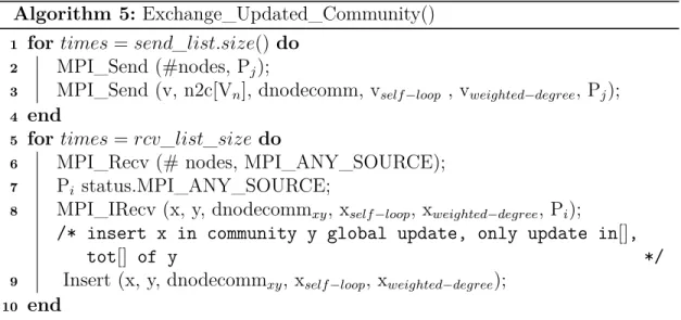
Algorithm 5: Exchange_Updated_Community()

1 for times =send_list.size()do

2 MPI_Send (#nodes, P_j);

3 MPI_Send (v, n2c[V_n], dnodecomm, vself−loop , vweighted−degree, Pj);

4 end

5 for times =rcv_list_size do

6 MPI_Recv (# nodes, MPI_ANY_SOURCE);

7 P_i status.MPI_ANY_SOURCE;

8 MPI_IRecv (x, y, dnodecommxy, xself−loop, xweighted−degree, Pi);

/* insert x in community y global update, only update in[],

tot[] of y */

9 Insert (x, y, dnodecommxy, xself−loop, xweighted−degree);

10 end

4.2.2.7 Resolving Community Duality

After the previous step, there remains an inconsistency to calculate total number of communities in the full network. The same network shown in Figure 4.1 is used to demonstrate the problem.

Table 4.2: Community Duality

Processor Vertex Community Problem Solution

P0 1 4 Vertex, 1 switched its community to vertex, 4 Vertex 1 retained community 4 P1 4 1 Vertex, 4 switched its community to vertex, 1 Vertex 4’s community switched back to vertex 4

Basically, Vertex 1 and Vertex 4 belong to the same community. It can be either 1 or 4. The community number does not have any effect on the result. But in current scenario, same community will be counted twice. So, we need to elim-inate this problem. To solve this, we kept the communities with higher number

and changed the lower numbers to higher ones. So now, in Table 4.2, vertex 4’s community is changed again to community 4 and vertex 1 retains its community 4. As, vertex 4 belongs to Processor 1. Processor 0 needs to communicate with it to circulate the update. In this step, we update the vertices’ communities those belong to current processor and track the communities those belonged to other processors and communication is required. So, for other processors those contain communities of the vertices, we summed the total number where current commu-nity id is less than vertex id and stored it in an array, count_commucommu-nity and it will be used in Step-8. We stored the vertices whose community will be updated after the communication. We also enlisted the unique community ids whose updated community we will receive after the communication is done. Both of these are required for the step described in Section 4.2.2.9.

4.2.2.8 Update of Processor List for Communication in Resolving Community Duality

This is a preliminary step required for Section 4.2.2.9. It is similar as described in Section 4.2.2.5. Here, we iterate over the array, count_community and stored the indices,i in send_list if count_community[i] > 0. i represents the processor number for sending. Update of receive list is also analogous to the calculation as described in Section 4.2.2.5 for finding out the size of receive_list.

4.2.2.9 Exchange of Duality Resolved Community

In this step, processor, Pi send to all processors, Pj from its send-list the

community-id to get the updated community of that id. Pj after receiving the message, sends back to Pi the corresponding community of received id. After receiving info from Pj, Pi updates the community of the vertices those needed

up-date, using the values from Section 4.2.2.7. In this communication step, subsequent send-receive is done.

Pimsg1

−−−→Pj where, j ∈send_list

msg13Community;Community ∈Pj

Pjmsg2 −−−→Pi

msg23Community, n2c[community];Community ∈Pj

A brief pseudo-code to represent Section 4.2.2.7, 4.2.2.9 is given in Algorithm 6.

Algorithm 6:Resolve_Community_Duality() and Exchange_Duality _Re-solved _Community()

1 for each vertex, v do 2 if n2c[v]< v then 3 if n2c[v] not in P_i then 4 P_j ← processor having n2c[v]; 5 MPI_Send(n2c[v],Pj); 6 MPI_Recv (n2c[v], n2c[n2c[v]], P_j); 7 n2c[v]←n2c[n2c[v]]; 8 else 9 comm←n2c[v]; 10 n2c[v]←n2c[comm]; 11 end 12 end 13 end

4.2.2.10 Finding Unique Communities and Computation of Modularity

In this step, each processor,Pi , where 0 <= i < N finds out all the unique communities by iterating over all of its vertices belonging to it.Pseudo-code is

Algorithm 7: Find_Unique_Communities() 1 Initialize empty array unique_community; 2 for each vertex, v do

3 comm←n2c[v];

4 if unique_community.contains()! =comm then

5 unique_community.push(comm);

6 end 7 end

To calculate total unique communities in the world, each Processor, Pk, where (1<=k<N) sends its unique_community list to root processor, P0. P0 then merges

all the unique communities received from each processor, Pk and eliminates dupli-cate ones.

Along with the unique_community list, Pkalso sends to P0values in1 and tot1

calculating the values from in and tot arrays. These two values are required for calculation of modularity of the full network. Algorithm 8 represents the pseudo-code for this step.

Algorithm 8: Compute_ Modularity() 1 if rank! = 0 then 2 i←rank; 3 m←total_weight; 4 in1← ( P_in[node] ) m ; 5 tot1←( P tot[node] m ) 2_;

6 MPI_Send(community array, in1i , tot1i, 0);

7 else

8 MPI_Recv (community array, in1_i ,tot1_i, MPI_ANY_SOURCE);

9 M odularity←Pin1₁−Ptot1_i;

4.2.2.11 Generating Next Level Graph

This step is performed by only the root processor, P0. P0 renumbers the

com-munities from 0 to Z −1 to formulate the new input graph to be used for next level.

Z = Total number of unique communities after merging and eliminating dupli-cate

So, Z is the number of vertices for input graph of next level. The connectivity of edges and corresponding weights are calculated from available data and the new graph is generated.

All the steps from Section 4.2.2.1 to 4.2.2.11 are done for each level of compu-tation and repeated as long as we get increase in modularity value.

4.3

Hybrid Parallel Louvain Algorithm

We use both MPI and OpenMP together to implement the Hybrid Parallel Lou-vain Algorithm. The hybrid version gives us the flexibility to balance between both shared and distributed memory system. We can tune between shared and distributed memory depending on available resources. In the multi-threading en-vironment, a single thread works for communication among processors and other threads do the computation.

4.4

Distributed Parallel Louvain Algorithm with

Load-balancing

To implement DPLAL, we use the similar approach as described in Section 4.2. In the first phase, we have used well-known graph-partitioner METIS [28] to

par-Algorithm 9: DPLAL-Distributed Parallel Louvain Algorithm using Load-balancing

Data: Input Graph G(V,E) [Edge List Format]

Result: (Vertex, Community) Pair 1 while increase in modularity do

2 G (V, E) is partitioned using METIS into p‘ partitions; 3 G‘(V,E) pre-processed according to METIS-Output;

4 G“(V,E) converted to Adjacency List format to be given to each processor ;

5 for Each processor Pi (executing in parallel) do

6 Gather_Neighbour_Info();

7 Compute_Community();

8 Exchange_Updated_Community();

9 Resolve_Community _Duality();

10 Exchange_Duality _Resolved _Community();

11 Find_Unique_Communities();

12 Compute_Modularity();

13 Generate_NextLevel_Graph();

14 if number_of_communities < i then

15 i← number_of_₂communities; 16 end

17 end 18 end

tition our input graph to distribute among the processors. Depending on METIS output, we adjust the number of processors because METIS does not always create same number of partitions as provided in input. We use both edge-cut and com-munication volume minimization approaches. An empirical comparison of these approaches is described later in Section 6. After partitioning, we distribute the input graph among the processors. For second phase, we follow the same flow as described in the Algorithm 1. But we have to recompute each function that has been calculated from input graph. Runtime analysis for each of these functions being used in MPI communication has been demonstrated in Section 6. Our incor-poration of graph partitioning scheme helps minimize the communication overhead of MPI to a great extent and we get an optimized performance from DPLAL.

Chapter 5

Experimental Setup

We describe our experimental setup and datasets below. We use large-scale com-pute cluster for working on large real-world graph datasets.

5.1

Execution Environment

We use Louisiana Optical Network Infrastructure (LONI) QB2 [29] compute clus-ter to perform all the experiments. QB2 is a 1.5 Petaflop peak performance clusclus-ter containing 504 compute nodes with over 10,000 Intel Xeon processing cores of 2.8 GHz. We use at most 50 computing nodes with 1000 processors for our experi-ments.

5.2

Description of Datasets

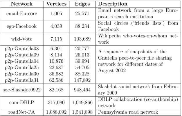
We have used real-world networks from SNAP [30] depicted in Table 5.1. We have performed our experimentation on different types of network including social networks, internet, peer-to-peer networks, road networks, network with ground truth communities, and Wikipedia networks. All these networks show different

structural and organizational properties. This gives us an opportunity to assess the performance of our algorithms for worst case inputs as well. The size of graphs used in our experiments ranges from several hundred thousands to millions of edges.

Table 5.1: Datasets used in our experimental evaluation.

Network Vertices Edges Description

email-Eu-core 1,005 25,571 Email network from a large

Euro-pean research institution

ego-Facebook 4,039 88,234 Social circles (’friends lists’) from Facebook

wiki-Vote 7,115 103,689 Wikipedia who-votes-on-whom

net-work

p2p-Gnutella08 6,301 20,777

A sequence of snapshots of the Gnutella peer-to-peer file sharing network for different dates of August 2002 p2p-Gnutella09 8,114 26,013 p2p-Gnutella04 10,876 39,994 p2p-Gnutella25 22,687 54,705 p2p-Gnutella30 36,682 88,328 p2p-Gnutella31 62,586 147,892

soc-Slashdot0922 82,168 948,464 Slashdot social network from Febru-ary 2009

com-DBLP 317,080 1,049,866 DBLP collaboration (co-authorship) network

Chapter 6

Results

We present the scalability and runtime analysis of our algorithms below. We discuss the trade-offs and challenges alongside.

6.1

Speedup factors of shared and distributed

memory algorithms

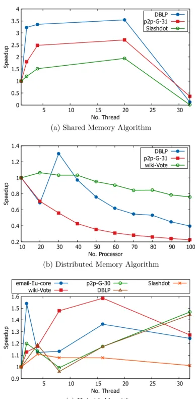
We design both shared and distributed memory based algorithms for Louvain meth-ods. The speedup results are shown in Fig. 6.1a and fig. 6.1b. Our shared memory and distributed memory based algorithms achieve speedups of around 4 and 1.5, respectively. The number of physical processing core available to our system is 20. Our shared memory algorithm scales well to this many cores. However, due to the unavailability of large shared memory system, we also design distributed memory algorithm. Further, shared memory algorithms show a limited scalability to large networks as discussed in [16]. Our distributed memory algorithm demonstrates only a minimal speedup for 30 processors . The inter-processor communication severely affects the speedup of this algorithm. We strive to overcome such

0 0.5 1 1.5 2 2.5 3 3.5 4 5 10 15 20 25 30 Sp ee du p No. Thread DBLP p2p-G-31 Slashdot

(a) Shared Memory Algorithm

0.2 0.4 0.6 0.8 1 1.2 1.4 10 20 30 40 50 60 70 80 90 100 Sp ee du p No. Processor DBLP p2p-G-31 wiki-Vote

(b) Distributed Memory Algorithm

0.9 1 1.1 1.2 1.3 1.4 1.5 1.6 5 10 15 20 25 30 Sp ee du p No. Thread email-Eu-core wiki-Vote p2p-G-30DBLP Slashdot (c) Hybrid Algorithm

Figure 6.1: Speedup factors of our parallel Louvain algorithms for different types of networks. Our hybrid algorithm strikes a balance between shared and distributed memory based algorithms.

munication bottleneck by designing hybrid algorithm.

6.2

Speedup factors of our hybrid parallel

algo-rithm

Our hybrid algorithm tends to find a balance between the above two approaches, shared and distributed memory. As shown in Fig. 6.1c, we get a speedup of around 2 for the hybrid implementation of Louvain algorithm. The speedup is similar to the MPI implementation. It is evident that in multi-threading environment run-time will decrease as workload is distributed among the threads. But we observe that in some cases, both single and multiple threads take similar time. Even some-times multiple threads take more time than a single thread. It indicates that hybrid implementation also suffers from the communication overhead problem alike MPI. Communication overhead of distributed memory setting limits the performance of hybrid algorithm as well.

6.3

Speedup factors of our improved parallel

al-gorithm DPLAL

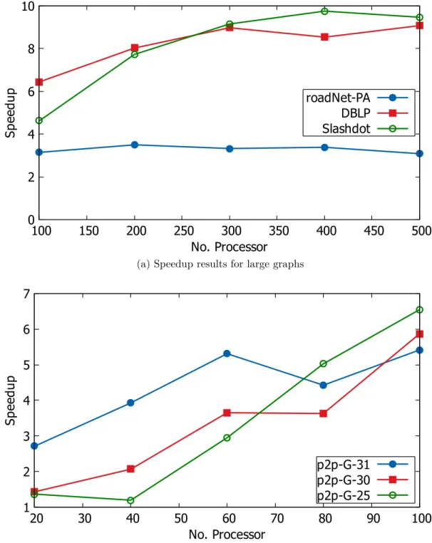
Our final parallel implementation of Louvain algorithm is DPLAL. This algorithm achieves a speedup factor up-to 12. We reduce the communication overhead in message passing setting to a great extent by introducing a load balancing scheme during graph partitioning. The improved speedup for DPLAL is presented in Fig-ure 6.2. For larger networks, our algorithm scales to a larger number of processors. We are able to use around a thousand processors. For smaller networks, the al-gorithm scales to a couple of hundred processors. It is understandable that for

0 2 4 6 8 10 100 150 200 250 300 350 400 450 500 Sp ee du p No. Processor roadNet-PA DBLP Slashdot

(a) Speedup results for large graphs

1 2 3 4 5 6 7 20 30 40 50 60 70 80 90 100 Sp ee du p No. Processor p2p-G-31 p2p-G-30 p2p-G-25

(b) Speedup results for relatively small graphs

Figure 6.2: Speedup factors of DPLAL algorithm for different types of networks. Larger networks scale to a larger number of processors.

smaller networks, the communication overhead gradually offsets the advantage ob-tained from parallel computation. However, since we want to use a larger number of processors to work on larger networks, our algorithm in fact has this desirable property. Overall, DPLAL algorithm scales well with the increase in the number of processors and to large networks.

6.4

Runtime analysis: a breakdown of execution

times

We present a breakdown of executions times. Fig. 6.3 shows the runtime anal-ysis for our largest network RoadNet-PA. We observe that communication time forgathering neighbor information and exchanging duality resolved community de-creases with increasing number of processors. Communication time for both ex-changing updated community and gathering updated community increases up-to a certain number of processors and after decreasing, the time becomes almost con-stant. Among all these communications, time to gather communities at the root processor takes maximum time and contribute to the high runtime.

6.5

Network size versus execution time.

For many large networks that we experimented on (including the ones in Fig. 6.2a), we find that those can scale to up to≈800 processors. We call this number as the optimum number of processors for those networks. This optimum number depends on network size. As our focus is on larger networks, to find out the relationship between runtime and network size, we keep the number of processor 800 fixed and run an experiment. As shown in Fig. 6.4, the communication

10

100

1000

10000

100000

100 200 300 400 500 600 700 800 900

40000

50000

60000

70000

80000

90000

100000

Ti

m

e

(m

s)

Ti

m

e

(m

s)

No. Processor

gathering neighbour info

exchanging updated community

exchanging duality resolved community

gathering updated communities

total duration

Figure 6.3: Runtime analysis of RoadNet-PA graph with DPLAL algorithm for varied number of processors. We show a breakdown of execution times for different modules or functions in the algorithm. Time for gathering updated communities and total duration are plotted w.r.t the righty-axis.

time forgathering neighbor info decreases with growing network size whereas both time forgathering updated communitiesandexchanging duality resolved community increase. Communication time forexchanging updated community increases up-to a certain point and then starts decreasing afterwards. For larger networks (>80K), total runtime increases proportionately with growing network size. As smaller graphs do not scale to 800 processors, these do not follow the trend, but it can be inferred that these will behave the same way for their optimum number of

processors.

1

10

100

1000

10000

100000

100000

1×10

Ti

m

e

(m

s)

Network Size

gathering neighbour info

exchanging updated community

exchanging duality resolved community

gathering updated communities

total duration

Figure 6.4: Increase in runtime of DPLAL algorithm with an increase in the sizes of the graphs keeping the number of processors fixed.

6.6

METIS partitioning approaches

We also compare the METIS partitioning techniques, between edge-cut and com-munication volume minimization, to find out the efficient approach for our algo-rithm. Fig. 6.5 shows the runtime comparison between edge-cut and communi-cation volume minimization techniques. We find that the communicommuni-cation volume

partitioning. So, in our subsequent experimentation, we have used edge-cut parti-tioning approach.

10000

100000

100 200 300 400 500 600 700 800 900

Ti

m

e

(m

s)

No. Processor

Edge-Cut (roadNetwork-PA)

Volume-Minimization (roadNetwork-PA)

Edge-Cut (DBLP)

Volume-Minimization (DBLP)

Edge-Cut (Slashdot)

Volume-Minimization (Slashdot)

Figure 6.5: Comparison of METIS partitioning approaches (edge-cut versus com-munication volume minimization) for several networks. The edge-cut approach achieves better runtime efficiency for the above real-world networks.

6.7

Performance Analysis

We present a comparative analysis of our algorithms, its sequential version, and another existing distributed memory algorithm.

6.7.1

Comparison with Other Parallel Algorithms

We compare the performance of DPLAL with another distributed memory parallel implementation of Louvain method given in Charith et al. [1]. For a network with 500,000 nodes, Charith et al. achieved a maximum speedup of 6 whereas with DPLAL for a network with 317,080 nodes we get a speedup of 12 using 800 processors. The largest network processed by them has 8M nodes and achieved a speedup of 4. Our largest network achieves a comparable speedup (4-fold speedup with 1M nodes). The work in [1] did not report runtime results so we could not compare our runtime with theirs directly. Their work reported scalability to only 16 processors whereas our algorithm is able to scale to almost a thousand of processors.

6.7.2

Comparison with Sequential Algorithm

We have compared our algorithms with the sequential version [15] to analyze the accuracy of our implementations. Deviation of the number of communities between sequential and our implementations is represented in Table 6.1. The deviation is negligible compared to network size. The number of communities is not constant and they vary because of the randomization introduced in the Louvain algorithm. Table 6.1 gives an approximation of the communities.

Although shared memory based parallel Louvain has the least deviation, the speed-up is not remarkable. Whereas, DPLAL shows a moderate deviation but its speedup is 3 times of that of shared parallel Louvain algorithm.

Table 6.1: Deviation of the number of communities for different parallel Louvain Algorithms from the sequential algorithm.

Algorithm Network com-DBLP wiki-Vote Comm. No. Dev. (%) Comm. No. Dev. (%) Sequential 109,104 - 1,213 -Shared 109,102 .0006 1,213 0 Distributed 109,441 0.106 1,216 0.042 Hybrid 104,668 1.39 1,163 0.71 DPLAL 109,063 0.0129 1,210 0.042

Chapter 7

Conclusion

Our parallel algorithms for Louvain method demonstrate good speedup on several types of real-world graphs. As instance, for DBLP graph with 0.3 million nodes, we get speedups of around 4, 1.5 and 2 for shared memory, distributed memory, and hybrid implementations, respectively. Among these three algorithms, shared memory parallel algorithm gives better speedup than others. However, shared memory system has limited number of physical cores and might not be able to process very large networks. A large network often requires distributed processing and each computing node stores and works with a part of the entire network. As we plan to work with networks with billions of nodes and edges, we work towards the improvement of the scalability of our algorithms by reducing the communica-tion overhead. We have identified the problems for each implementacommunica-tion and come up with an optimized implementation DPLAL. With our improved algorithm DPLAL, community detection in DBLP network achieves a 12-fold speedup. Our largest network, roadNetwork-PA has 4-fold speedup for same number of proces-sors. With increasing network size, number of processor also increases. We will work with larger networks increasing the number of processors in our future work.

also experiment with other load-balancing schemes to find an efficient load balanc-ing scheme to make DPLAL more scalable. We also want to eliminate the effect of small communities that create misconception to understand the community struc-ture and its properties. Further, we will explore the effect of node ordering (e.g., degree based ordering, random ordering) on the performance of parallel Louvain algorithms.

Bibliography

[1] C. Wickramaarachchi, M. Frincuy, P. Small, and V. Prasannay, “Fast parallel algorithm for unfolding of communities in large graphs,” inHigh Performance Extreme Computing Conference (HPEC), 2014 IEEE, pp. 1–6, IEEE, 2014. [2] S. Arifuzzaman and M. Khan, “Fast parallel conversion of edge list to

adja-cency list for large-scale graphs,” in Proceedings of the 23rd Symposium on High Performance Computing 2015, pp. 17–24, Society for Computer Simula-tion InternaSimula-tional, 2015.

[3] S. Arifuzzaman, M. Khan, and M. Marathe, “Patric: A parallel algorithm for counting triangles in massive networks,” in Proceedings of the 22nd ACM international conference on Information & Knowledge Management, pp. 529– 538, ACM, 2013.

[4] S. Arifuzzaman and B. Pandey, “Scalable mining and analysis of protein-protein interaction networks,” in 3rd Intl Conf on Big Data Intelligence and Computing (DataCom 2017), pp. 1098–1105, IEEE, 2017.

[5] M. Girvan and M. E. Newman, “Community structure in social and biological networks,” Proceedings of the national academy of sciences, vol. 99, no. 12, pp. 7821–7826, 2002.

[6] H. Kwak, C. Lee, H. Park, and S. Moon, “What is twitter, a social network or a news media?,” inProceedings of the 19th international conference on World wide web, pp. 591–600, AcM, 2010.

[7] J. Ugander, B. Karrer, L. Backstrom, and C. Marlow, “The anatomy of the facebook social graph,”arXiv preprint arXiv:1111.4503, 2011.

[8] S. Arifuzzaman, M. Khan, and M. Marathe, “A space-efficient parallel algo-rithm for counting exact triangles in massive networks,” in 2015 IEEE 17th International Conference on High Performance Computing and Communica-tions (HPCC), pp. 527–534, IEEE, 2015.

[9] S. Arifuzzaman, M. Khan, and M. Marathe, “A fast parallel algorithm for counting triangles in graphs using dynamic load balancing,” in 2015 IEEE International Conference on Big Data (Big Data), pp. 1839–1847, IEEE, 2015. [10] J. D. McCalpin et al., “Memory bandwidth and machine balance in current high performance computers,”IEEE computer society technical committee on computer architecture (TCCA) newsletter, vol. 1995, pp. 19–25, 1995.

[11] N. S. Sattar and S. Arifuzzaman, “Parallelizing louvain algorithm: Distributed memory challenges,” in2018 IEEE 16th Intl Conf on Dependable, Autonomic and Secure Computing (DASC 2018), pp. 695–701, IEEE, 2018.

[12] N. Talukder and M. J. Zaki, “Parallel graph mining with dynamic load bal-ancing,” in Big Data (Big Data), 2016 IEEE International Conference on, pp. 3352–3359, IEEE, 2016.

[13] A. Raval, R. Nasre, V. Kumar, S. Vadhiyar, K. Pingali, et al., “Dynamic load balancing strategies for graph applications on gpus,” arXiv preprint arXiv:1711.00231, 2017.

[14] N. S. Sattar and S. Arifuzzaman, “Overcoming mpi communication overhead for distributed community detection,” inWorkshop on Software Challenges to Exascale Computing, pp. 77–90, Springer, 2018.

[15] V. D. Blondel, J.-L. Guillaume, R. Lambiotte, and E. Lefebvre, “Fast un-folding of communities in large networks,” Journal of statistical mechanics: theory and experiment, vol. 2008, no. 10, p. P10008, 2008.

[16] S. Bhowmick and S. Srinivasan, “A template for parallelizing the louvain method for modularity maximization,” inDynamics On and Of Complex Net-works, Volume 2, pp. 111–124, New York: Springer, 2013.

[17] C. L. Staudt and H. Meyerhenke, “Engineering parallel algorithms for com-munity detection in massive networks,” IEEE Transactions on Parallel & Distributed Systems, no. 1, pp. 1–1, 2016.

[18] A. Lancichinetti and S. Fortunato, “Community detection algorithms: a com-parative analysis,”Physical review E, vol. 80, no. 5, p. 056117, 2009.

[19] A. Clauset, M. E. Newman, and C. Moore, “Finding community structure in very large networks,”Physical review E, vol. 70, no. 6, p. 066111, 2004. [20] U. N. Raghavan, R. Albert, and S. Kumara, “Near linear time algorithm

to detect community structures in large-scale networks,” Physical review E, vol. 76, no. 3, p. 036106, 2007.

[21] J. Leskovec, K. J. Lang, and M. Mahoney, “Empirical comparison of algo-rithms for network community detection,” in Proceedings of the 19th interna-tional conference on World wide web, pp. 631–640, ACM, 2010.

[22] M. Fazlali, E. Moradi, and H. T. Malazi, “Adaptive parallel louvain commu-nity detection on a multicore platform,” Microprocessors and Microsystems, vol. 54, pp. 26–34, 2017.

[23] “Cray documentation portal.” https://pubs.cray.com/

content/S-3014/3.0.UP00/cray-graph-engine-user-guide/ community-detection-parallel-louvain-method-plm.

[24] E. Moradi, M. Fazlali, and H. T. Malazi, “Fast parallel community detection algorithm based on modularity,” in 2015 18th CSI International Symposium on Computer Architecture and Digital Systems (CADS), pp. 1–4, IEEE, 2015. [25] H. Lu, M. Halappanavar, and A. Kalyanaraman, “Parallel heuristics for

scal-able community detection,”Parallel Computing, vol. 47, pp. 19–37, 2015. [26] M. Halappanavar, H. Lu, A. Kalyanaraman, and A. Tumeo, “Scalable static

and dynamic community detection using grappolo,” inHigh Performance Ex-treme Computing Conference (HPEC), 2017 IEEE, pp. 1–6, IEEE, 2017. [27] S. Ghosh, M. Halappanavar, A. Tumeo, A. Kalyanaraman, H. Lu,

D. Chavarria-Miranda, A. Khan, and A. Gebremedhin, “Distributed louvain algorithm for graph community detection,” in2018 IEEE International Paral-lel and Distributed Processing Symposium (IPDPS), pp. 885–895, IEEE, 2018. [28] “Metis - serial graph partitioning and fill-reducing matrix ordering|karypis

lab.” http://glaros.dtc.umn.edu/gkhome/metis/metis/overview.

[29] “Documentation | user guides | qb2.” http://www.hpc.lsu.edu/docs/ guides.php?system=QB2.

[30] “Stanford large network dataset collection.” https://snap.stanford.edu/ data/index.html.

Vita

Naw Safrin Sattar

Naw Safrin Sattar obtained her Bachelor0s degree in Computer Science and En-gineering from Bangladesh University of EnEn-gineering and Technology (BUET) in 2016. She joined the University of New Orleans Computer Science Graduate pro-gram to pursue a PhD in the field of Big Data Analytics and High Performance Computing in Fall 2017. She is working as a Graduate Reseach Assistant in the Big Data and Scalable Computing Research Group under the supervision of Dr. Shaikh Arifuzzaman. Her research interest includes Big Data Analytics, High Per-formance Computing, Graph Mining & Analysis, and Parallel Algorithms.