Bard College Bard College
Bard Digital Commons
Bard Digital Commons
Senior Projects Spring 2016 Bard Undergraduate Senior Projects
Spring 2016
Radical Recognition in Off-Line Handwritten Chinese Characters
Radical Recognition in Off-Line Handwritten Chinese Characters
Using Non-Negative Matrix Factorization
Using Non-Negative Matrix Factorization
Xiangying ShuaiBard College, [email protected]
Follow this and additional works at: https://digitalcommons.bard.edu/senproj_s2016
Part of the Applied Linguistics Commons, Applied Mathematics Commons, Applied Statistics Commons, Artificial Intelligence and Robotics Commons, Computational Linguistics Commons, and the Graphics and Human Computer Interfaces Commons
This work is licensed under a Creative Commons Attribution-Noncommercial-No Derivative Works 4.0 License.
Recommended Citation Recommended Citation
Shuai, Xiangying, "Radical Recognition in Off-Line Handwritten Chinese Characters Using Non-Negative Matrix Factorization" (2016). Senior Projects Spring 2016. 367.
https://digitalcommons.bard.edu/senproj_s2016/367 This Open Access work is protected by copyright and/or related rights. It has been provided to you by Bard College's Stevenson Library with permission from the rights-holder(s). You are free to use this work in any way that is permitted by the copyright and related rights. For other uses you need to obtain permission from the rights-holder(s) directly, unless additional rights are indicated by a Creative Commons license in the record and/or on the work itself. For more information, please contact
Radical Recognition in Off-Line
Handwritten Chinese Characters Using
Non-Negative Matrix Factorization
A Senior Project submitted to
The Division of Science, Mathematics, and Computing
of
Bard College
by
Xiangying (Shar) Shuai
Annandale-on-Hudson, New York
May, 2016
Abstract
In the past decade, handwritten Chinese character recognition has received renewed inter-est with the emergence of touch screen devices. Other popular applications include on-line Chinese character dictionary look-up and visual translation in mobile phone applications. Due to the complex structure of Chinese characters, this classification task is not exactly an easy one, as it involves knowledge from mathematics, computer science, and linguistics. Given a large image database of handwritten character data, the goal of my senior project is to use Non-Negative Matrix Factorization (NMF), a recent method for finding a suit-able representation (parts-based representation) of image data, to detect specific sub-components in Chinese characters. NMF has only been applied to typed (printed) Chinese characters in different fonts. This project focuses specifically on how well NMF works on handwritten characters. In addition, research in Chinese character classification has mainly been done using holistic approaches - treating each character as an inseparable unit. By using NMF, this project takes a different approach by focusing on a more specific problem in Chinese character classification: radical (sub-component) detection.
Finally, a possible application of radical detection will be proposed. This interactive ap-plication can potentially help Chinese language learners better recognize characters by radicals.
Abstract 1
Dedication 6
Acknowledgments 7
1 Introduction 8
1.1 What is Character Recognition . . . 8
1.2 Chinese Characters and the Significance of Radicals . . . 9
1.3 Databases of Handwritten Chinese . . . 11
1.4 Simple Approaches . . . 12
1.4.1 Hamming Distance . . . 12
1.4.2 Scale Invariant Feature Transform . . . 13
2 Radical Extraction Using Matrix Factorization 15 2.1 Non-Negative Matrix Factorization . . . 15
2.1.1 The Basic NMF Algorithm in Detail . . . 16
2.1.2 NMF Applications . . . 21
2.1.3 Outline of Radical Detection Using NMF . . . 23
2.2 NMF Results . . . 25
2.2.1 Preliminary Results . . . 26
2.2.2 The Learning Curves of NMF . . . 27
2.2.3 Statistical Comparisons of Two Pairs of Algorithms . . . 31
3 Conclusion 36 3.1 Discussions and Comparisons . . . 36
Contents 3
3.3 Conclusion . . . 40
3.4 Future Work . . . 41
3.4.1 Constrained Sparse Matrix Factorization . . . 41
3.4.2 Affine Sparse Non-Negative Matrix Factorization . . . 43
Appendix A Map of Radicals to GB2312 45 Appendix B Brief Descriptions of the NMF Variants 48 B.0.3 Probabilistic Model (PMF) . . . 48
B.0.4 Alternating Least Squares with Projected Gradient (LSNMF) . . . . 48
B.0.5 Non-smooth Model (NSNMF) . . . 49
B.0.6 Enforced Sparseness (SNMF) . . . 49
B.0.7 Penalized Model (PMFCC) . . . 50
Appendix C Plots of Learning Curves 51
Appendix D Paired Comparisons of Means and Variances 54
Appendix E Python Code for Radical Classification 59
1.2.1 Hierarchical Composition of a Chinese Character . . . 9
1.3.1 HIT-OR3C Data Example . . . 11
1.4.1 Poor Alignment of Characters in Hamming Distance . . . 13
1.4.2 SIFT Code Example . . . 14
1.4.3 Incorrect Feature Detection by SIFT . . . 14
2.1.1 Reconstruction of a Face Using NMF . . . 21
2.1.2 Visualization of NMF . . . 22
2.1.3 Illustration of the Training and Testing Phases . . . 23
2.1.4 An Example of a Reconstructed Character . . . 24
2.2.1 Distribution of Radicals Over the Count of Characters (Character Variability) 28 3.2.1 Dictionary Look-Up Drawing Application . . . 39
3.2.2 A Proposed Layout for a Character Learning Application . . . 39
3.4.1 Normalization of Data . . . 43
C.0.1Learning Curves . . . 52
C.0.2Scaled Learning Curves . . . 53
D.0.1Paired Mean Accuracy and Variance Comparison between Standard NMF and SNMF (First Half) . . . 55
D.0.2Paired Mean Accuracy and Variance Comparison between Standard NMF and SNMF (Second Half) . . . 56
D.0.3Paired Mean Accuracy and Variance Comparison between Standard NMF and Penalized NMF (First Half) . . . 57
D.0.4Paired Mean Accuracy and Variance Comparison between Standard NMF and Penalized NMF (Second Half) . . . 58
List of Tables
2.1.1 Use of Parameters in Different NMF Applications . . . 22 2.2.1 Results from Different NMF Variants Using a Minimum Training Set . . . . 26 2.2.2 Results from Different NMF Variants After Studying the Learning Curves . 30 2.2.3 t-Test for Population Means - Standard NMF and SNMF . . . 34 2.2.4 F-Test for Population Variances - Standard NMF and SNMF . . . 34 2.2.5 t-Test for Population Means - Standard NMF and Penalized NMF . . . 35 2.2.6 F-Test for Population Variances - Standard NMF and Penalized NMF . . . 35
I would like to dedicate this project to all of my family members - my grandparents in both China and the U.S., Chunxiu Tao, Guangcai Shuai, Amy and Jim Delaune Sr., my uncle, Gang Shuai, and my parents, Jim and Sophie Delaune. I am so very grateful for your guidance, support, and generosity all these years. Thank you!
Acknowledgments
First and foremost, I would like to thank my senior project advisers Amir Barghi and Sven Anderson for providing extraordinary guidance, support, patience, energy and en-couragement not just this past year, but also throughout my time at Bard. Being a joint major is extremely difficult, and I want to thank both Sven and Amir for always being there for me. Without them, I would not have graduated with a joint degree. I also want to thank my senior project board members, Keith O’Hara and Ethan Bloch for their in-valuable suggestions and encouragement. Also, I want to thank Sven and Ethan for giving me much encouragement as my academic advisers.
Furthermore, I want to thank Dean Bethany Nohlgren, Dean Mary Ann Krisa, and Fu-chen Chan for being such inspirational mentors this year. I also want to thank Dean Rebecca Thomas for being a wonderful role model - her success stories have strengthened my belief that as a woman I can be successful in S.T.E.M.
Lastly, I want to thank Kathleen (Katie) Burke, Alexandra Morris, and Marley Alford for being such inspirational co-clubheads of Women in S.T.E.M. @ Bard with me this year. I believe we have made a difference and will continue to make differences in improving gender equality in the S.T.E.M. fields.
1
Introduction
1.1
What is Character Recognition
Character recognition, or optical character recognition, is a field of research in computer vision, pattern recognition, and artificial intelligence that endeavors to recognize hand-written characters using computer algorithms. With the emergence of touch screen de-vices, the field of handwritten character recognition has received renewed interest in the past few years. Other related popular applications include signature verification, writer identification, on-line dictionary look-up, visual translation in mobile phone applications, etc.
In the research field of handwritten character recognition, “off-line” and “on-line” are important terms that describe the form of the data. The on-line case refers to the avail-ability of trajectory data during the time of data collection, and the off-line case refers to data in the form of scanned images, or data in the form of pixels of images.
In this paper, we focus on Chinese characters due to their complex hierarchical struc-ture and rich variations. Only off-line data is used in this project because real-time live user interaction is not required. Furthermore, this project focuses specifically on
detect-1. INTRODUCTION 9 ing radicals/sub-components in Chinese characters, since this is a relatively unexplored problem.
1.2
Chinese Characters and the Significance of Radicals
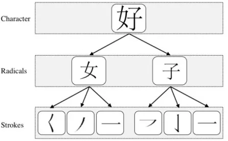
The Chinese writing system is extremely hierarchical: words consist of individual charac-ters, which in turn consist of a group of radicals (“偏旁部首”, sub-components), which then in turn consist of a sequence of strokes (“笔划”, the simplest components of each character). In general, a single Chinese character stands for at least one meaning, while a radical can also carry some semantic clues of the character. For example, the character “好”(hǎo, meaning “good”), consists of the two radicals “女” (nǚ, meaning “female”, or “daughter”), and “子” (zǐ, meaning “son”). Figure 1.2.1 demonstrates how a Chinese character can be decomposed based on the “character-radical-stroke” hierarchical law.
Figure 1.2.1.Hierarchical Composition of a Chinese Character: Every character can be decomposed based
on the
“character-radical-stroke” hierarchical law.
For example, the character
“好”consists of the two
radi-cals “女”, and “子”, which in
turn consist of a sequence of six simple strokes.
There are three known general approaches to Chinese character recognition: holistic, stroke-based, and radical-based.
Holistic Approaches: Most studies are done using holistic approaches, which recog-nize each character as an indivisible unit. No segmentation is performed and the whole character is recognized at once [15]. If we were to recognize characters holistically, we
would need to determine the size of the entire Chinese character set. According to statis-tics [11], there are over 400,000 unique Chinese characters, where 4,000 are used on a daily basis. If we were to classify them holistically and individually, the scale of usage obviously challenges holistic classification methods because naturally, even with the help of a good classification algorithm, the probability of selecting a correct character out of 4,000 is very small.
Stroke-Based Approaches: Another popular approach is to base classification on the extraction of low-level features such as strokes. Stroke-based methods focus on de-composing each character into a set of strokes, and then classify it based on the number, position, order, shape and orientation of the set of strokes [15]. However, because there are many variations (size, degree orientation, position, etc) of each type of stroke, this method essentially also has to deal with the problem of a large number of features. In addition, stroke-extraction is extremely difficult if a particular style of handwriting merges several strokes into continuous curves (similar to cursive handwriting in western languages). On the other hand, stroke-based approaches can be explored with on-line data since stroke order information would be available.
Radical-Based Approaches: Lastly, radical-based approaches decompose each char-acter into its sub-components, or radicals, and classify the charchar-acter based on the com-bination of the radicals and their positions within that character. There are 214 unique radicals in Chinese script, which is relatively small compared to the set of commonly used characters. Moreover, unlike strokes, each radical would only have one or two variations (vertical or horizontal). However, there are only a few existing methods that have focused on radical decomposition. Ideally, recognizing radicals is much easier than recognizing the whole character or its individual strokes. A native Chinese speaker recognizes characters based on high-level features such as the radicals (because they often contribute to the
1. INTRODUCTION 11 meaning of the character), rather than low-level features such as the strokes. These obser-vations motivate us to research on radical-based approaches to classify Chinese characters.
1.3
Databases of Handwritten Chinese
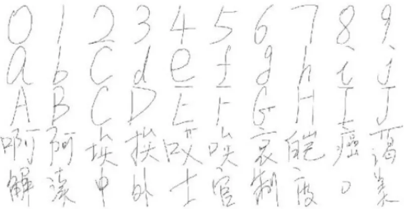
There are several databases of handwritten Chinese characters on-line, such as the CASIA On-line and Off-line Chinese Handwriting Databases built by the National Laboratory of Pattern Recognition (NLPR) and the Institute of Automation of Chinese Academy of Sci-ences (CASIA) [1]. In this study, we will use a relatively smaller but more recent database known as the Harbin Institute of Technology Opening Recognition Corpus for Chinese Characters (HIT-OR3C), which was collected in 2010 [4]. A sample of the data is shown in Figure 1.3.1.
Figure 1.3.1. HIT-OR3C Data Example
The HIT-OR3C contains both on-line and off-line data of 6,825 unique classes, collected from 122 different writers, with 832,650 samples in total. The 6,825 character classes correspond to the 6,825 characters in the Guojia Biaozhun 2312 (GB2312, “国家标准”) table, which is the registered name for a key official character set of China, used for simplified Chinese characters. The GB2312 table covers 99.75% of the characters used for daily Chinese input.
Furthermore, the 6,825 character classes are divided into two main sections: characters in the first section are arranged according to Pinyin (“拼音”, the Chinese alphabet), and characters in the second section are arranged according to radicals (in increasing strokes). In this project, only the 3008 character classes in the second half of the data are used since the goal is to find radicals in the characters [4]. A complete mapping from radical classes to the characters in GB2312 can be found in Appendix A [2]. However, the map shows that only 168 out of the 214 radical classes are used in the second section of the data set. In the HIT-OR3C data set, all the Chinese characters have been collected using a tablet with a handwriting document collection software: OR3C Toolkit, which is available for download on the website. The original individual character images are 128 by 128 grey scale.
In our off-line character recognition experiments, the image samples are converted to 128 by 128 binary matrices by averaging the RGB values of each pixel and setting a threshold of 128. That is, an average pixel value of less than 128 is considered as background and is converted to 0. Otherwise, it is considered as foreground and converted to 1. The data is converted to binary because the recognition methods we explore work well with sparse data, as explained in the next chapter.
1.4
Simple Approaches
1.4.1 Hamming Distance
Previously, we talked about how holistic approaches are quite challenging because of the large character class size. The most common and simple holistic approach in character recognition problems is template matching, where individual pixels are used as features. Classification is performed by comparing an input character with a set of templates (or prototypes) from each character class. Each comparison results in a similarity measure between an input character and a template.
1. INTRODUCTION 13 We will show one holistic approach that fails to classify characters - Hamming distance, which compares the matrices of two character images and finds the number of positions at which the corresponding binary values are different. Hence, the smaller the Hamming distance is between two characters, the more similar they are to each other. To do so, we generated a set of 6,825 typed characters (which are used as templates/prototypes) cor-responding to the GB2312 table, and for each input handwritten character, we calculated the Hamming distance between the input and each typed character, and picked the typed character that was “closest” to the input. We tested this method using 5,000 randomly picked input characters, and the accuracy rate was less than 1%. The explanation for the low classification rate is simple - poor alignment, as shown in Figure 1.4.1.
Figure 1.4.1. Poor Alignment of Charac-ters in Hamming Distance: Simply matching handwritten characters with printed template characters results in poor alignment issues, as printed characters do not demonstrate most of the variations in handwritten characters: size, orientation, stroke density, and differences in handwriting.
Handwritten characters in general vary in size, orientation, and density, especially when there are multiple writers. Hence a simple holistic method such as this will not capture the similarities between handwritten characters.
1.4.2 Scale Invariant Feature Transform
There are some much more sophisticated methods to detect features in images, such as Scale-Invariant Feature Transform (SIFT). Hence we used SIFT to see how well it detects features in each character. A major part of SIFT is image feature generation, which trans-forms an image into a large collection of feature vectors, each of which is invariant to image translation, scaling, and rotation, partially invariant to illumination changes and robust to local geometric distortion. Fortunately, OpenCV (a library of computer vision functions)
has built-in SIFT functions to detect key points in images [6]. Figure 1.4.2 demonstrates how to use the OpenCV SIFT function to detect interesting points in an image [6].
Figure 1.4.2. SIFT Code Example. The code demonstrates how interesting features are detected in a given image. First it reads the input image and turns it into grayscale, and then it detects the points and draws them on an output image.
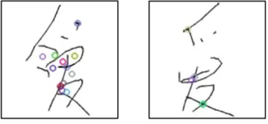
Figure 1.4.3 is an example of how SIFT fails to detect the same key points for two images of the same character (“爱”, love) written by just two different people.
Figure 1.4.3. Incorrect Feature Detection by SIFT. The figure shows the key points detected in the same character written by two different people. It is clear that the key points in each image not only differ in the number, but also in the locations.
Poor classification results from the above experiments using holistic approaches do not show that all holistic approaches are not suitable for Chinese character recognition, nor that they are not effective. Rather, the results show the drawback of these approaches, that they require a high degree of correlation between the test and training images. In addition, holistic methods do not perform effectively under large variations in direction, scale and handwriting style. In the following chapter, we will explore a new radical-based method: non-negative sparse matrix factorization for automatically extracting radicals from Chinese characters.
2
Radical Extraction Using Matrix Factorization
2.1
Non-Negative Matrix Factorization
A fundamental problem in many pattern recognition tasks such as ours is finding a suit-able representation of the data. Non-Negative Matrix Factorization (NMF), is a recently developed method for finding such a representation [3]. The NMF method has been used for many data analysis tasks such as face decomposition, font classification, gene expres-sion clustering, and scalable Internet distance (round-trip time) prediction.
The NMF method was originally proposed by Lee and Seung to find parts of individ-ual objects: “Non-negative matrix factorization is distinguished from other methods by its use of non-negativity constraints. These constraints lead to a parts-based representa-tion because they allow only additive, not subtractive, combinarepresenta-tions.” By contrast, other methods, such as principal component analysis and vector quantization, learn holistic, not parts-based, data representations [9].
Definition 2.1.1. Given ann×m non-negative input matrixV, a Non-Negative Matrix Factorization is one that aims to decompose it into an n×r basis matrix W, and r×m
and H as follows Vij ≈(W H)ij = r X a=1 WiaHaj = ˆVij,
where the rank r of the factorization is generally picked so that (n+m)r < nm,W ≥0,
and H≥0. 4
2.1.1 The Basic NMF Algorithm in Detail
The goal of the NMF algorithm is to decompose an input matrixV into a basis setW and encoding setH specified in Definition 2.1.1, while satisfying the non-negativity constraint. We will talk about what W and H each represents in the context of radical detection in the next section.
To approximate W and H, the NMF algorithm first initiates two random positive ma-trices of dimensionsn×rand r×m, respectively. The next step is to repeatedly calculate the difference between the estimated matrix ˆV =W H and the input matrixV, and at the same time update the elements in both W and H to minimize this difference iteratively, until some kind of a convergence criteria is met - the maximum number of iteration steps is reached, or the total errorE is less than a predefined error threshold.
To converge V and W H is to minimize the construction error ||V −W H||2, which is
the squared error (Euclidean distance) between V and W H. The general error function
E, known as Frobenius Norm, can be described as follows:
E(W, H) = 1 2||V −W H|| 2 F = 1 2 X ij (Vij −(W H)ij)2. (2.1.1)
Furthermore, the element-wise error betweenV and ˆV is:
Eij(W, H) = 1 2||Vij −Vˆij|| 2 F = 1 2(Vij− r X a=1 WiaHaj)2. (2.1.2)
The above error terms are squared because the difference between the actual input matrix and the estimated matrix can be either positive or negative.
2. RADICAL EXTRACTION USING MATRIX FACTORIZATION 17 In order to minimize the error, we need to know either to increase or decrease the current element values inW andH. Generally speaking, to find a local minimum of a function, one needs to take steps proportional to the opposite/negative direction of the gradient of the cost function at each iteration, and this method is known as Gradient Descent. Hence in our case, to find the directions of element values inW andH, we differentiate the function in (2.1.2) with respect to any pair of elements Wik and Hkj (such that WikHkj = ˆVij)
separately [19]: ∂ ∂Wik Eij = 1 2 ∂ ∂Wik (Vij − r X a=1 WiaHaj)2 =−(Vij−Vˆij)(Hkj) =−EijHkj. (2.1.3) ∂ ∂Hkj Eij = 1 2 ∂ ∂Hkj (Vij − r X a=1 WiaHaj)2 =−(Vij−Vˆij)(Wik) =−EijWik. (2.1.4)
Notice that in (2.1.3), the partial derivative of (Vij −Pra=1WiaHaj) with respect to any
Wik inW is only one term,−Hkj, not a sum. This is becauseWik only corresponds to one of the terms in Pra=1WiaHaj, where 1≤k≤r. Hence the other terms witha6=k cancel
out in the derivation process. This explanation applies to (2.1.4) as well.
Having formulated the gradient for any pair of elementsWik andHkj, we can now take
a step proportional to the opposite of the gradients and derive the update rules for them separately: Wik0 =Wik+α ∂ ∂WikEij =Wik+αEijHkj. (2.1.5) Hkj0 =Hkj+α ∂ ∂Hkj Eij =Hkj+αEijWik, (2.1.6)
In common Gradient Descent and linear regression problems,αis known as the “learning rate” whose value determines the rate the algorithm is approaching the local minimum at each iteration. Usually a very small value (such as 0.001) is chosen because we want to take small steps towards each local minimum to avoid the risk of missing it.
So far we have described a set of simple additive update rules, (2.1.5) and (2.1.10). A more popular approach, proposed by Lee and Seung [9] is to update the matrices multiplicatively [9]: Wik0 ←Wik (V HT)ik (W HHT) ik (2.1.7) and Hkj0 ←Hkj (W TV) kj (WTW H) kj . (2.1.8)
The major advantage of the multiplicative approach is, as long as the initiation process of the matrices assigns positive values to all elements, multiplying each matrix element by a positive value makes sure the new element is also positive. In addition, there is no learning parameterα to tune.
The multiplicative rules can easily be derived from the additive ones. First, we will rewrite the additive update rules in (2.1.5) and (2.1.10) into the following forms:
Wik0 =Wik+α ∂ ∂Wik Eij =Wik+α ∂ ∂Wik (Vij − r X a=1 WiaHaj)2 =Wik+α(Vij−WikHkj)(Hkj)
=Wik+α(VijHikT −WikHkjHikT) =Wik+α(V HT −W HHT)ik
(2.1.9)
2. RADICAL EXTRACTION USING MATRIX FACTORIZATION 19 Hkj0 =Hkj+α ∂ ∂HkjEij =Hkj+α ∂ ∂Hkj (Vij− r X a=1 WiaHaj)2 =Hkj+α(Vij−WikHkj)(Wik) =Hkj+α(WkjTVij−WkjTWikHkj) =Hkj+α(WTV −WTW H)kj. (2.1.10)
Next, Lee and Seung proposed to replace the αin rule (2.1.9) with the following term:
α= Wik (W HHT)
ik
, (2.1.11)
and rule (2.1.9) is then rewritten into rule (2.1.7):
Wik0 =Wik+α(V HT −W HHT)ik =Wik+ Wik (W HHT) ik (V HT −W HHT)ik =Wik+ Wik (W HHT) ik (V HT)ik− Wik (W HHT) ik (W HHT)ik =Wik+Wik (V HT)ik (W HHT) ik −Wik =Wik (V HT)ik (W HHT) ik . (2.1.12)
Similarly, theα in rule (2.1.10) can be replaced by substituting the following term:
α= Hkj (WTW H)
kj
, (2.1.13)
Hkj0 =Hkj+α(WTV −WTW H)kj =Hkj+ Hkj (WTW H) kj (WTV −WTW H)kj =Hkj+ Hkj (WTW H) kj (WTV)kj − Hkj (WTW H) kj (WTW H)kj =Hkj+Hkj (WTV)kj (WTW H) kj −Hkj =Hkj (WTV) kj (WTW H) kj . (2.1.14)
Finally, a pseudo code for the NMF can be found in Algorithm 2.1.1. Lee and Seung have proved that the algorithm under update rules (2.1.7) and (2.1.8) is guaranteed to reach at least a locally optimal solution [9].
Algorithm 1 NMF Algorithm
1: procedure Init 2: initialize W+ 3: initialize H+
4: procedure Factorize
5: for iteration inmaxNumberOfIterationsdo
6: forrow=i,col=j inV do
7: compute Eij
8: compute gradients ∂Wik∂ Eij and ∂Hkj∂ Eij 9: calculate updated elements Wik0 andHik0 10: compute total error E
11: if E <errThresholdthen
12: break
13:
return W,H
In the above algorithm, “maxNumberOfIterations”, the maximum number of iterations the algorithm will run is generally specified by the user. “errThreshold”, the tolerance threshold for the total error at each iteration, is also used to decide when to stop updating the elements. This value is usually set to a very small positive number to ensure a close approximation of ˆV toV.
2. RADICAL EXTRACTION USING MATRIX FACTORIZATION 21
2.1.2 NMF Applications
In recent years, researchers have applied NMF to various problems. Among the most well-known applications are face decomposition, font classification, and document classification. The most original application of NMF is face decomposition - looking for localized features that correspond with intuitive notions of the parts of faces (the eyes, the nose, and the mouth) [9]. Now let’s take another look at NMF based on Definition 2.1.1. The dimensions of each matrix can be expressed as follows:
V[n×m]≈W[n×r]×H[r×m].
In Lee and Seung’s research, the image database of faces is regarded as ann×mmatrix
V, with each column being an input image in the form of a size-n vector. There are m
input images in total. The r columns of W are called basis images, and each column of
H is called an encoding and has a one-to-one relationship with each face in V. What is even more important to know is that an encoding consists of the coefficients by which a particular face image is represented with a linear combinations of the basis images of
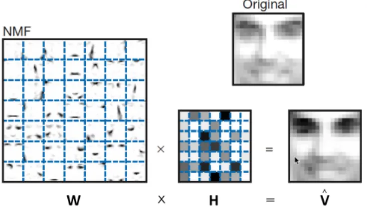
W [9]. Once W and H are approximated, they can be used to reconstruct a new face, as demonstrated in Figure 2.1.1 [9].
W x H = V >︎
Figure 2.1.1. Reconstruction of a face using NMF. Non-negative matrix factoriza-tion learns a parts-based representafactoriza-tion of
faces: the W shown here is a set of r =
72= 49 basis images (the eyes, the nose, the
mouth, etc). A particular test image, tagged as “Original” here, is approximately repre-sented by a linear superposition of the
im-ages inW, with encodings inH (the darker
the color the bigger the coefficient matrix el-ement is).
As can be seen from Figure 2.1.1, a large fraction ofW, the NMF image basis, consists of vanishing coefficients. Hence both the basis images and image encodings are sparse
(see Definition 2.1.2). The basis images are sparse because they are not global, and they represent various versions of facial features, mouths, noses, eyes, etc, in different locations and forms. Any face in the data can be generated by combining these different parts, but the combination does not necessarily need all of these basis images [9] .
Definition 2.1.2. A sparse matrix is a matrix in which most of the elements are zero. By contrast, if most of the elements are nonzero, then the matrix is considered dense. 4
Based on the above idea, many other applications including Chinese character classifica-tion can use NMF to decompose data into different features. Figure 2.1.2 and Table 2.1.2 summarize some of these applications.
Figure 2.1.2. Visualization of NMF
Application n m r
Face Decomposition Total number of pixels in
an image.
Number of face image samples.
Number of different facial features.
Font Classification Total number of pixels in a
letter/character image of a specific font.
Number of character image samples.
Number of different fonts.
Chinese Radical Detection
Total number of pixels in a character image. In this
project,n= 1282.
Number of character image samples.
Number of different radical classes.
Table 2.1.1. Use of Parameters in Different NMF Applications
The following section will explain in detail how NMF can be used to detect radicals in Chinese characters.
2. RADICAL EXTRACTION USING MATRIX FACTORIZATION 23
2.1.3 Outline of Radical Detection Using NMF
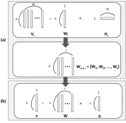
Tan, Xie, Zheng, and Lai were the first to use NMF on Chinese characters, and more specifically, they used the method to find radicals in printed characters. Unlike handwritten characters, the only variation in printed characters is the font [15]. Their method can be illustrated as below in two phases - training and testing, as shown in Figure 2.1.3.
Figure 2.1.3. Illustration of the Training and Testing Phases. In (a), the training phase, each
radical Wi is learned using m
characters (in their column vec-tor form) that contain the
radi-cal.WiandHiare estimated to
best fitVi. When all 168 radicals
have been learned, together they
form the radical dictionary, W.
Then in (b), the testing phase,
for every test imagev,Wis used
to estimate h, a one-column
co-efficient matrix, which is used to determine what radicals are most prominent in the reconstruction
ofv.
In general NMF applications, theW matrix is known as a dictionary, and in this prob-lem, it is known as a radical dictionary. Each column ofW represents a basis radical class [15]. In other NMF applications where the features are unknown,ris usually estimated in order to better approximateW andH. In this problem, we specify r= 1 at each training step, because we want to isolate radical classes in order to learn them individually. As demonstrated in Figure 2.1.3, in the training phase (a), we train each radical class Wi
separately from the others using NMF, with m characters that contain this radical. The training is done when we haver column vectors trained for the r= 168 radical classes in
the data. Then W stays constant and is passed into (b), the testing phase. Each column ofW corresponds to one of the learned radical classes. Hence each testing character image (in its column vector form), can again be estimated as:
v≈W ×h, (2.1.15)
where W is known, and h is a coefficient matrix that is estimated using least squares (because W is not a square matrix, we cannot solve forh using the inverse of W). Since most characters are structured by no more than four or five components, and eachhi∈h
represents how important a radical class i in W is in the formation of a character, we can see if particular radicals exist in a character simply by examining the top four or five coefficients in h. In this paper, we make the assumption that all characters have no more than five components. Figure 2.1.4 demonstrates how a character in the testing phase can be reconstructed using the estimated W and H.
Figure 2.1.4. An Example of
a Reconstructed Character: As
demonstrated, the input character
“刈(y`ı, [verb] to regulate)” is used
as a testing image sample. In this example, only five radical classes are used in the radical dictionary
W for demonstration purposes,
with “刂” being the first radical
class in W. The coefficient matrix
hcorrectly predicted that the most
prominent sub-component in “刈” is
“刂” (the peak atx= 0). Although
the left part of the reconstructed image appears to be a blur (since
it contains radical classes that
are not learned), the right side
clearly demonstrates that “刂” is a
2. RADICAL EXTRACTION USING MATRIX FACTORIZATION 25
2.2
NMF Results
In this section, we will record the initial results of radical detection using the following variants of NMF: standard, probabilistic, projected gradient, non-smooth, sparse (imposed on the W matrix), sparse (imposed on the H matrix), and penalized NMF. A short description of each NMF variant (except standard NMF, which is previously described in depth in Section 2.1.1) can be found in Appendix B. These are the most popular NMF methods used today. Since NMF has not been applied to handwritten character classification, we want to apply all of these methods to see which algorithms would produce good results.
The basis for comparison at this point is only the average accuracy over all radical classes. After we get a general idea of how each variant algorithm performs, we will then compare some of the algorithms in depth in the following section.
Another idea we want to explore here is how the accuracy of NMF changes as a function of the training-set size. As seen in Appendix A, not all radical classes map to the same number of characters (we will refer the number of characters a radical class maps to as
its character variability). For example, radical class number 4, “儿(´er, son)”, only maps
to itself, where as radical class number 24, “阝(ˇer, ear)”, maps to 61 characters, such as “阢”, “阡”, “阱”, “阪”, “阽”, “阼”, etc. Hence for a radical class such as “儿”, we get 1 character sample from each of the 122 writers in the data, leading to a total of only 122 samples representing the radical class (hence it has very little noise in the training set). On the other hand, “阝” would have 122×61 = 7442 samples (which we assume would lead to more noise in the training set). Hence, different radical classes might require training sets of different sizes for them to be better represented in the dictionary.
2.2.1 Preliminary Results
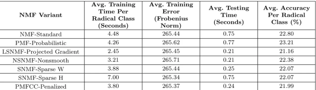
To explore how the accuracy is related to the training set size, we need to first establish a basis for comparison, using a minimum training set that is equal for all radical classes. For each radical class, we pick only 102 random samples from the pool of all 122 writers, and the testing phase will test on the remaining 20 samples. This way, all the radical classes are learned on training sets of equal size.
We will then use the seven variants of NMF to see how the results differ. It is impor-tant to state that there is no overlap between the training and testing image samples. In addition, for each variant NMF algorithm we use, the experiment is run 10 times (using identical training and testing sets for each algorithm) and returns the average measure-ments. The results are recorded below in Table 2.2.1. The average training and testing times are useful measures calculated to determine the efficiency of the various NMF algo-rithms. The training error, known as Frobenius Norm, is our error function described in Equation 2.1.1. NMF Variant Avg. Training Time Per Radical Class (Seconds) Avg. Training Error (Frobenius Norm) Avg. Testing Time (Seconds) Avg. Accuracy Per Radical Class (%) NMF-Standard 4.48 265.44 0.75 22.80 PMF-Probabilistic 4.26 265.62 0.77 23.21 LSNMF-Projected Gradient 2.45 265.45 0.21 21.16 NSNMF-Nonsmooth 3.21 265.71 0.21 22.38 SNMF-Sparse W 3.88 265.44 0.25 22.07 SNMF-Sparse H 7.00 265.34 0.75 22.07 PMFCC-Penalized 3.80 265.37 0.24 21.99
Table 2.2.1. Results from Different NMF Variants Using a Minimum Training Set
All of the results shown in Table 2.2.1 suggest the poor performance of NMF when using the same number of samples to train each radical class. Because of the small training set size, the W dictionary is not a good representation of character variability.
rad-2. RADICAL EXTRACTION USING MATRIX FACTORIZATION 27 ical would lead to a better representation of character variability. To answer this question, we used standard NMF to train on all available data, and tested the resulting dictionary on the same testing samples used above (20 testing samples per radical class), and obtained an average classification accuracy of 27.08% over 10 runs. By using all of the available data to learn the radical, the average classification accuracy improved by less than 5%. It is possible that this is the best result, but it is more likely that using all of the available data impacts the dictionary’s ability to generalize the radical classes and their features -that by using all of the data, too much irrelevant variation is added to the training set. This is quite a common issue in machine learning.
In the following subsection, we will make use of a concept known as learning curves to see if incrementally increasing the training size (yet without using the entire data set) will affect the results in a positive way. Plotting the learning curves for the radical classes can show us how to fit the data efficiently.
2.2.2 The Learning Curves of NMF
A learning curve is a measure of predictive performance on a given domain as a function of varying amounts of learning effort. The most common form of learning curves in machine learning shows predictive accuracy on the testing samples as a function of the number of training samples. In this radical recognition problem, the accuracy for each radical class might vary depending on the number of training samples we use. The more training samples we use, the more variations of characters are added to the training set. This improves the generalization of the dictionary due to observing more character variability. One idea is to group all of the radical classes into equal subsets and plot learning curves for each subset. Note that it is impossible to graph a learning curve for each radical class, as we need a substantial number of radicals in a dictionary to determine the efficiency of the algorithm. Because a radical exists in a test character if it is one the top five coefficients
of h, aW matrix with r = 1 (r is the number of radicals/columns in the W dictionary) is extremely biased and would definitely always return a classification accuracy of 100%. Hence it is important each subset contains more than 5 radical classes.
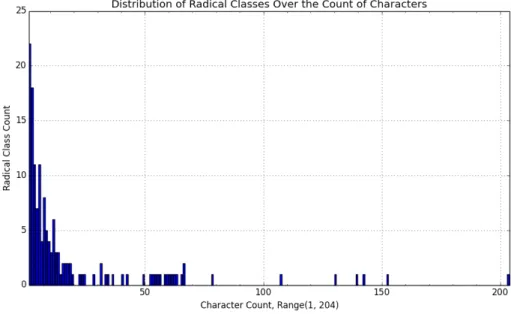
First we need to see the distribution of the 3008 characters among the 168 radical classes. Let R={r1, r2, . . . , r168} be the set of 168 radical classes such that radical class
ri maps to |ri| characters. Appendix A shows that the smallest|ri| is 1, and the largest |ri|is 204. We plotP168
i=1ri such that|ri|=x for allx∈[1,204]. That is, each column in
the graph represents the number of radical classes that map to x characters. The sum of all the columns is 168 as we have 168 radical classes.
Figure 2.2.1.Distribution of Radicals Over the Count of Characters (Character Variability): The x-axis represents the number of characters a radical class maps to (character variability), and the y-axis shows the sum of the radical
classes that map toxcharacters. It is shown that most radical classes map to fewer than 50 characters, while there
are only a few radical classes that map to more than 100 characters.
Figure 2.2.1 shows that most radical classes map to fewer than 50 characters, while there are only a few radicals that map to more than 100 characters. We cannot plot the learning curves for radical classes that contain fewer than 5 characters, because the range is not wide enough to show improvement in accuracy. This excludes 197 characters out of
2. RADICAL EXTRACTION USING MATRIX FACTORIZATION 29 the set of 3008 characters. We then group the rest of the elements inR (adding the bars by multiplying them with their corresponding x value in Figure 2.2.1 in a left-to-right fashion) into three subsets of equal size, S1, S2, and S3. Hence when we test a random
character in a certain radical class, the probability of that radical being already trained in any one of the three subsets is equal.
After grouping the three subsets, we find that |S1| ≈ |S2| ≈ |S2| ≈ 1
3(3008−197), and S1={ri ∈R | 5<|ri| ≤42} S2={ri ∈R | 43<|ri| ≤78} S3={ri ∈R | |ri| ≥79}.
In a sense, S1 can be thought of as a subset of radical classes that have low character
variability (all of them map to less than 42 characters). Similarly, radical classes inS2have
medium character variability, and radical classes in S3 have high character variability.
We also double-checked that each subset contains more than 5 radical classes. Now we have extracted the domains to plot the learning curve for each subset. Since each character is written by 122 different writers, it means each character sample has 122 copies. We can use 102 of those for training and 20 for testing. Hence each number in the domain is actually multiplied by 102 in training. The resulting learning curves are shown in Appendix C.
The learning curve for S1 shows that using around 300 samples for training is ideal
for radical classes in S1. The S2 and S3 learning curves are not minimally monotonous
(they contain many peaks), but they show some peaks which can still suggest some good numbers to use for training. The highest peaks arex≈1400 and x≈1900 forS2 and S3,
respectively. It is clear that radical classes with high character variability require more training samples than the ones with low character variability.
our observations from the learning curves, Ni can be determined as follows: Ni = |ri| ×102 if|ri| ≤5 3×10² if 5<|ri| ≤42 14×102 if 43≤ |ri| ≤78 19×102 otherwise (|ri| ≥79),
where for |ri| ≤ 5, all of radical class ri’s available training samples are used. It is im-portant to emphasize that partitioning the 3008 characters into three equal subsets (in increasing character variability) is only one way to plot the learning curves. While our partitioning methodology yields good results (shown below), other methods might also lead to improvement in learning, such as forming subsets of radical classes with similar number of strokes, or making sure each subset has the same number of radical classes.
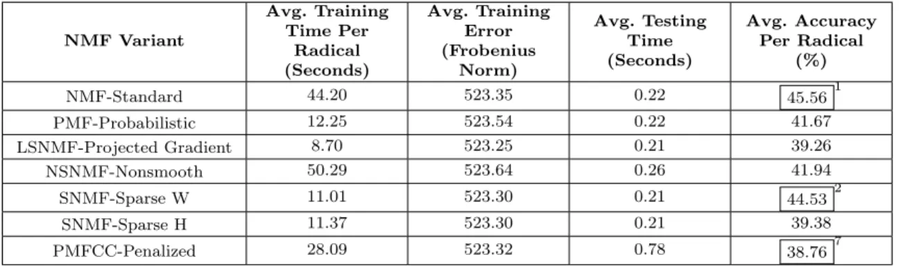
By using the above partition and the 7 NMF variants for training, we get the results in Table 2.2.2 from testing on 3,360 character images (exactly 20 characters from each of the 168 radicals). Appendix E contains our Python code for radical classification using the training data partitioning methodology described in this section.
NMF Variant Avg. Training Time Per Radical (Seconds) Avg. Training Error (Frobenius Norm) Avg. Testing Time (Seconds) Avg. Accuracy Per Radical (%) NMF-Standard 44.20 523.35 0.22 45.561 PMF-Probabilistic 12.25 523.54 0.22 41.67 LSNMF-Projected Gradient 8.70 523.25 0.21 39.26 NSNMF-Nonsmooth 50.29 523.64 0.26 41.94 SNMF-Sparse W 11.01 523.30 0.21 44.532 SNMF-Sparse H 11.37 523.30 0.21 39.38 PMFCC-Penalized 28.09 523.32 0.78 38.767
Table 2.2.2. Results from Different NMF Variants After Studying the Learning Curves. We boxed and ranked the accuracies of the top two and also the least efficient algorithms.
The above results show significant improvement in accuracy compared to the ones listed in Table 2.2.1. It is clear that using more training samples generally leads to better results because a higher level of character variability is expressed.
2. RADICAL EXTRACTION USING MATRIX FACTORIZATION 31 training time does not matter significantly even though the training times for the 7 algo-rithms vary greatly. Hence we can say that the differences between the training errors are negligible. All of the testing times are under one second. Hence the differences are also not significant. What we need to focus on is the accuracy - Standard NMF and SNMF (with imposed sparsity on W) show similar accuracies, whereas the penalized model shows the lowest accuracy. In the next subsection, we will analyze how statistically different these results are.
2.2.3 Statistical Comparisons of Two Pairs of Algorithms
In machine learning, an overall classification accuracy alone is typically not enough infor-mation to help determine what is the best algorithm. The slight difference we saw in the accuracies produced by Standard NMF and SNMF might be a result of the variance in the training or testing data and other reasons. In this problem, since our classification system consists of as many as 168 classes, we cannot use common measurements such as a con-fusion matrix or a ROC (receiver operating characteristic curve, which is used for binary classification) to examine the performance of NMF. However, we can apply two commonly used statistical methods on our NMF results: One-Sample Paired t-Test for Population Means and One-Sample Paired F-Test for Population Variances. We will first apply the two tests once to the standard NMF and SNMF pair, to see how statistically different the two best algorithm results are. Then we will apply the two tests to the standard NMF and penalized NMF pair, to see how statistically different the best and the worst algorithm results differ.
Standard NMF & SNMF - One-Sample Paired t-Test for Population Means:
The paired sets of data would be the two sets of accuracies provided by the two NMF algorithms. Each set contains 168 averaged accuracies, one for each radical class.
Let X be the set of accuracies returned by Standard NMF, and Y be the set of ac-curacies returned by SNMF. Since we want to see if the average results are significantly different, we want to set up two hypotheses to examine the accuracies. The null hypothesis is that the overall means of the two sets of results are equal:
H0 :X−Y = 0 (2.2.1)
The alternative hypothesis is that there is a difference in the overall means of the two sets of results:
H1 :X−Y 6= 0 (2.2.2)
The first step of the t-test is to calculate the difference (Di =Yi−Xi) between the two observations on each of the N = 168 pairs. Calculating the mean (D) and the square of standard deviation value (s2D) of the differences gives:
D= P iDi N ≈0.0104 (2.2.3) and SD2 = P iD2i N−1 − N(D)2 N−1 ≈0.0526. (2.2.4) Then, the standard error of the mean difference (SE(D)) is:
SE(D) = √SD
N ≈0.0513, (2.2.5)
and the test statistic tratio is found from:
t= D
SE(D) ≈0.2003, (2.2.6) with N −1 = 167 degrees of freedom under the null hypothesis. Using the t-value, we can find thep-value (probability distribution) using thept command inR (a software for statistical computing):
2. RADICAL EXTRACTION USING MATRIX FACTORIZATION 33 Suppose we use a significance level of α = 0.05 in this test, we have p > α, which means we cannot reject the null hypothesis,H0. This means there is insufficient evidence
to conclude that the two sets of results have different means.
Although the overall improvement of NMF over SNMF in average accuracy is only 1%, it is not a negligiable difference. It would be useful to calculate a confidence interval for the mean difference to tell us within what limits the true difference is likely to lie. A 95% confidence interval for the true mean difference is:
D±tα/2×SE(D), (2.2.8)
where tα/2 is the 2.5% point of the t-distribution on N −1 = 167 degrees of freedom. UsingR again, we can find that the confidence interval is:
[−0.0245,0.0453], (2.2.9)
which means if we do the same experiment to compare NMF and SNMF 100 times, 95 times the true value for the average difference would lie in the 95% confidence interval shown above.
Standard NMF & SNMF - One-Sample Paired F-Test for Population
Vari-ances:To build a more solid analysis of the difference between the two sets of results, we can also compare their variances, σX2 for SNMF andσ2Y for NMF. To do so, we can make the following hypothesis:
H00 :σX2 −σ2Y = 0 (2.2.10)
and
H00 :σX2 −σY2 6= 0. (2.2.11)
Suppose we choose a significance level of α= 0.05 again. The test statisticF is:
F = S 2 X SY2 ≈ 0.22082 0.26032 ≈ 0.0488 0.0678 ≈0.7198. (2.2.12)
Then using R again, we can find the probability distribution for theF-statistic is:
p≈0.0091, (2.2.13)
which means, with 95% confidence, the null hypothesis H00 is rejected. Furthermore, we find that the confidence interval for the difference in the two population variances is:
[0.4917,0.9039]. (2.2.14)
That is, we are 95% confident that the ratio of the two population variances is between 0.4917 and 0.9039. Since the interval does not contain the ratio value 1, we can conclude that the population variances differ. Table 2.2.3 and Table 2.2.3 sum up the comparisons between the two algorithms.
Table 2.2.3. t-Test for Population Means - Standard NMF and SNMF t-value N-1 Significance (α) p-value Confidence Interval Difference 0.2003 167 0.05 0.5793 [-0.0245, 0.0453]
Table 2.2.4. F-Test for Population Variances - Standard NMF and SNMF F-value N-1 Significance (α) p-value Confidence Interval Difference 0.7198 167 0.05 0.0091 [0.4917, 0.9039]
Based on the above tests, we can conclude that although there is insufficient evidence to conclude which algorithm yields a better overall accuracy, we see that there is lower variance among the average accuracies of the radical classes in standard NMF. That is, the 168 accuracies in SNMF disperse further from their population mean than those of NMF. As described in Appendix B, SNMF imposes sparseness (more zero elements) on
W. It is possible that the level of sparseness is uneven among the radical classes (columns) inW, leading to more variance among the performance of its radicals.
In conclusion, standard NMF should be used if there there is a preference for accuracies closer to the expected values, whereas SNMF (with imposed sparseness onW) can be used
2. RADICAL EXTRACTION USING MATRIX FACTORIZATION 35 when there is a preference in a shorter training time.
Standard NMF & Penalized NMF - One-Sample Paired t-Test for Population
Means and F-Test for Population Variances: We will follow the same calculations described previously to derive the two test statistics for standard NMF and penalized NMF. The details are omited and we will just show the results in Tables 2.2.3 and 2.2.3.
Table 2.2.5. t-Test for Population Means - Standard NMF and Penalized NMF t-value N-1 Significance (α) p-value Confidence Interval Difference 0.7137 167 0.05 0.7618 [0.0031, 0.1330]
Table 2.2.6. F-Test for Population Variances - Standard NMF and Penalized NMF F-value N-1 Significance (α) p-value Confidence Interval Difference 1.7138 167 0.05 1.663e-07 [1.6786, 3.0854]
Again, the One-Sample Paired t-Test shows that we cannot reject the null hypothesis that the populations means of standard NMF and penalized NMF are the same. There is insufficient evidence to conclude that the two sets of results have different means. What we can conclude is that the standard NMF results are much more variant than that of penalized results.
Appendix D contains plots that compare the means and variances of all 168 radical classes between the two pairs of algorithms: standard NMF and SNMF (the two best algorithms), and standard NMF and penalized NMF (the best and the worst). Figure D.0.1 and Figure D.0.2 are great illustrations that show although standard NMF and SNMF yield similar accuracies among all radical classes, there is greater variance among the performance of radical classes in SNMF. Furthermore, Figure D.0.3 and Figure D.0.4 demonstrate that although there is greater variance among the performance of individual radicals in standard NMF, it yields much better results than the penalized method.
3
Conclusion
3.1
Discussions and Comparisons
Among the existing methods for handwritten Chinese character classification, the radical-based approach may be the most similar to human cognition, given that most native Chinese speakers recognize characters by their radicals (because they give semantic clues about the meanings of the characters). However, radical extraction in Chinese characters is still relatively unexplored because of the challenges it presents. In this paper, we used Non-Negative Matrix Factorization (NMF) to extract the radicals in handwritten charac-ters. NMF is a very recent methodology proposed to find “parts-based” representation of objects (usually imagery or textual objects). This method had only been previously used on printed characters [15].
In this paper, we find that learning each radical using a training set with a size deter-mined based on the radical’s character variability (the number of characters it maps to) yields better results than using a minimum or maximum training set. After learning all 168 radicals (as column vectors), a radical dictionary matrix is formed, which we can use to predict what radicals are present in new testing image samples. Furthermore, because
3. CONCLUSION 37 we did not know which NMF variants would yield good results, we used seven different variants of NMF (including the standard one) to learn the dictionary. Based on the average classification accuracies (using the same training and testing samples for all algorithms over 10 runs/executions), we find that the standard NMF algorithm and Sparse NMF (with an imposed sparseness on the dictionary matrix) yield the best results. While the standard algorithm performs well on all radicals, the individual radical class performance in SNMF shows more variance.
Without modifying the input data images, Non-Negative Matrix Factorization already produces positive results (a 45% accuracy rate and a testing time that is less than a sec-ond) that exceed our expectations, also given that the data has so many variations (size, rotation, and different handwriting styles). We believe that with some modifications in the data itself, NMF will perform more efficiently.
The original research (by Tan, Xie, Zheng, and Lai) that applied NMF to printed Chi-nese characters made two more modifications: Taking away the non-negative constraint and normalizing all images to a bounding shape (which we will describe in the future work section) [15]. Their methods produced a character classification rate of 99.2%. It is difficult to compare our results with theirs since they focused on character classifica-tion and we focused on radical classificaclassifica-tion. However, since they assumed each character has at most two radicals, we can estimate their radical classification rate to be approxi-mately√99.2%≈99.6% (assuming that both radicals in each character are independent), which is a lot better than ours. On the other hand, the scale of their experiments was much smaller. They learned only 59 radicals from 648 printed characters, and used only 1029 testing samples. It is natural that classification of handwritten characters is more challenging than that of printed characters because of the handwriting style variations in handwritten characters.
The author, Daming Shi, reported a radical classification rate of 96.5% and a character classification rate of 93.5%. His experiments were conducted using 200 radical classes on a test set of 430,800 characters from 2,154 character classes [13] (whereas we used 168 radicals, 3,360 testing samples from 3008 character classes), which is on a much larger scale than ours and produced much better results. Shi’s approach is entirely different. For training, he uses kernel principle-component analysis to find “landmark” points in the training samples and capture the main variations around the mean radical. He makes the assumption that each character consists of up to four unique radicals. For testing, chamfer distance minimization is used to match radicals within a character using the dynamic tunneling algorithm to search for the best shape parameters to describe the deformation of an active model to fit the test image [13]. The author used a combination of algorithms to best capture the many variations in Chinese characters.
Based on the above comparisons, it is clear that although the standard NMF algorithm already produces meaningful results on handwritten characters produced by different writ-ers, alone it is not enough to produce comparable results. Nevertheless, it has been proved that NMF performs well in finding parts and sub-components of objects. Furthermore, radical classification can be used in many useful real-world applications, and we will make a proposal for one in the following section.
3.2
A Proposal for a Character Learning Application
As mentioned in the introductory sections, handwritten Chinese character recognition has received renewed interest with the emergence of touch screen devices. An on-line dictionary called Line Dictionary, which bills itself as “more than a dictionary”, has a handy feature that allows users to find Chinese characters by drawing them with a mouse, a track pad or a tablet. Figure 3.2.1 is an illustration of the feature [10].
3. CONCLUSION 39
Figure 3.2.1.Dictionary Look-Up Drawing Applica-tion. This on-line application allows the user to draw a character using a mouse, and then it makes sugges-tions in real time about what that character might be. The example shown here is a hand drawn character,
好(good), and it is clear that the application makes a
correct prediction.
Unlike English, the sound (Pinyin) of a Chinese character does not correlate with its shape, and to type a character, one must know its sound. The application in Figure 3.2.1 is useful when the user does not know the Pinyin of the character, which happens frequently to non-native speakers. While an application like this is becoming more and more popular, there still does not exist a similar application that extracts radicals from a hand drawn character. Thereby we will make a proposal for such an application here (Due to time constraints, we will not be able to actually implement the idea). We propose the following layout for the radical learning application:
Figure 3.2.2. A Proposed Layout for a Character Learning Application. We model the new application based on the layout of the previous one, with an additional “Next Page” button to allow the user to look at more options.
The initial step of building the application requires that we learn the radical dictionary
W beforehand and save the matrix into a file. Then, whenever a user finishes writing, we convert the character image into a matrix of binary elements. Next, we useW to estimate
the coefficient matrix h, pick the top 12 coefficients in h, and display the corresponding radicals. Finally, when the user picks the desired radicals, the application should display the following information about the radical: meaning, number of strokes, etc.
We model the new application based on the layout of the previous one, with an addi-tional “Next Page” button to allow the user to look at more options. Recall that in our experiment, we defined that a radical is found in a testing sample if its index appears to be in the top five elements of the estimated coefficient matrix,h. The layout of the proposed application allows there to be at least 12 suggestions of radicals, and the user is allowed to look at more suggestions if the desired radicals are not on the first page. This means the actually radical classification rate might be much higher than 45%. However, when building and testing the model, we still need to take into account of new styles of hand-writing being introduced to the testing set. One solution is to update the W dictionary constantly as new styles of handwriting appear.
3.3
Conclusion
In this project, we used a novel approach known as Non-Negative Matrix Factorization (NMF), a recent method for finding a suitable parts-based representation of imagery data, to detect sub-components (known as radical characters) in handwritten Chinese characters. Whereas most researchers focus on holistic approaches, by using NMF, this project takes a different approach and a human cognitive perspective by focusing on a more specific problem - radical detection.
In our experiments, seven variants of the NMF algorithm were used to learn a dictionary that represents 168 radical classes. We find that learning each radical using a training set of a size most suitable to represent its character variability produces better results than using a minimum or maximum training set. Furthermore, by testing on 3,360 character image samples, the best accuracies are 45.56% and 44.53%, produced by standard NMF
3. CONCLUSION 41 and sparse NMF (SNMF, with enforced sparseness on the dictionary matrix), respectively. We have also found that while standard NMF performs well on all radical classes, SNMF is much faster and shows more variance. We assume the variance is a result of uneven sparseness among the learned radical classes.
Finally, we proposed a character learning model which can potentially be built into a mobile phone or web application. The application would allow the user to first hand draw a Chinese character, then it predicts what radicals may be present in the character image, and after the user selects the desired radicals, the application displays the following information about the chosen radicals: meaning, number of strokes, etc. From a linguistic point of view, we believe that learning radicals and their shapes and meanings would help a learner better recognize Chinese characters and memorize their meanings.
NMF has shown to be a dynamic method that produces meaningful results for many different types of problems. For future study, it would be interesting to see NMF being applied to other Eastern Asian languages that also have hierarchical character structures, such as Korean and Japanese.
3.4
Future Work
The researchers that applied NMF to printed Chinese characters also proposed two mod-ification of the problem: changing the non-negative constraint in NMF, and normalizing the input data using Affine transform. We will briefly describe these two proposals in the following subsections.
3.4.1 Constrained Sparse Matrix Factorization
Due to the non-negative restraint, NMF meets many challenges and requirements in real applications. In Tan, Xie, and Zheng’s study, they propose to drop the non-negative con-straint, because although it may affect the sparseness, is unnecessary for character
de-composition [15]. They introduced Constrained Sparse Matrix Factorization (CSMF) as an improvement of NMF. CSMF guarantees the sparseness by dropping the non-negative constraint, and at the same time it brings in penalized functions. Usually, penalty terms are added to the new method in order to replace a constrained optimization problem by unconstrained problems whose solutions ideally converge to the solution of the original constrained problem.
In CMSF, V corresponds to the character set, W corresponds to the radical set, and
H is a matrix of unique decomposition coefficients specific toV and with respect to basis
W [15]. Finding the point of convergence between V and W H in CMSF is the same as NMF - we need to minimize the construction error||V−W H||2, which is the squared error
(Euclidean distance) betweenV and W H. Then the CSMF can be described as follows:
minW,HE(W, H) = 1 2||V −W H|| 2 F +g1(W) +g2(H) (3.4.1) s.t.W ∈D1, H ∈D2
where D1 and D2 are domains of W and H, andg1 and g2 are penalized functions ofW
and H, respectively [15] [18]. The penalty functions are described as follows:
g1(W) =α r X j1=1 r X j2=1 n X c,j26=j1 |Wj1(c)||Wj2(c)|+β r X j=1 n X c=1 |Wj(c)|, (3.4.2) and g2(H) =λ m X k=1 r X j=1 |hk(j)|, (3.4.3) s.t. W ∈Rn×r, W ≥0 andH ∈Rr×m
whereα, β, andλare non-negative weights/coefficients specifying the importance of each term [15] [18]. It is easy to see that CSMF evolves from NMF because whenD1={W ≥0},
D2={H≥0}and α=β =λ= 0, CSMF is essentially NMF.
3. CONCLUSION 43 terms are placed where the original constraints are violated to compensate for the violation. Ideally, the solutions of the unconstrained problems will eventually converge to that of the original constrained problem.
3.4.2 Affine Sparse Non-Negative Matrix Factorization
Because of the complexity of Chinese characters, and the variations of handwriting in our data set, NMF might not perform well as it may result in radical extraction variations in location, scale, or direction. To overcome this problem, Tan, Xie, Zheng, and Lai proposed to apply Affine transformation on all characters in the date set, and called this modified method Affine Sparse Matrix Factorization (ASMF) [15].
The Affine transformation procedure can be seen as the normalization step of the data set, so that all characters in the data set can have an identical shape, which is bounded by a rectangle and resembles a TBLR quadrilateral, as shown in Figure 3.4.1. [15].
Figure 3.4.1.Normalization of Data: (a) Bound-ing rectangle, (b) TBLR quadrilateral.
ASMF Overview: Letf denote the Affine transformation. Then we can combine the previously described CSMF with Affine transformation and propose the following ASMF definition: min W∈D1,H∈D2E(W, H) = 1 2||A−W H|| 2 F +g1(W) +g2(H) =||f(V)−W H||2+g1(W) +g2(H) (3.4.4) where Aiu=f(Viu)≈(W H)iu= r X a=1 WiaHau
and D1,D2,g1 and g2 are described in the previous section.
Now the Affine tranformation can be described as follows:
Ai=f(Vi) =AVi+b=AsAtAuAθVi+b = s 0 0 s 1 0 1 t 1 u 0 1 cos(θ) −sin(θ) sin(θ) cos(θ) Vi+ b1 b2 b3 b4 =
s·cos(θ) (stu)·cos(θ)−(st)·sin(θ)
s·sin(θ) (stu)·sin(θ)−(st)·cos(θ)
Vi+ b1 b2 b3 b4 , (3.4.5)
whereAs,At,Au,Aθ, andbdenote the scaling, stretching, skew, rotation, and translation parameters, respectively. The Affine transformation will improve the alignment of charac-ters by adjusting them into a common normal structure.
For future work, it would be interesting to see if the modifications that work well on printed characters would also improve NMF’s performance on handwritten characters.
Appendix A
Map of Radicals to GB2312
The following is a radical index for the 3,008 GB 2312-80 Level 2 hanzi, arranged according to a reduced set of 186 radicals (this index also applies to GB/T 12345-90 Level 2 hanzi). The GB 2312-80 Row-Cell codes for the radicals themselves are also provided under the “Radical”column. Note that some radicals do not have a corresponding range—hanzi categorized under such radicals are in GB 2312-80 Level 1 hanzi.
Number Radical GB 2312-80 1 50-27 c 5601–5612 2 56-13 丨 5613–5614 3 56-15 丿 5615–5627 4 56-28 丶 5628 5 50-50 乙 5629–5632 6 22-94 二 5633 7 42-14 十 5634–5637 8 19-07 厂 5638–5645 9 56-46 匚 5646–5651 10 18-23 卜 5652–5653 11 56-54 刂 5654–5670 12 56-71 冂 5671–5672 13 56-73 亻 5673–5757 14 40-43 人 5758–5765 15 16-43 八 5766–5771 16 57-72 勹 5772–5775 17 28-24 几 5776–5777 18 22-89 儿 5778 19 57-79 亠 5779–5790 20 57-91 冫 5791–5801 21 58-02 冖 5802–5804 Number Radical GB 2312-80 22 58-05讠 5805–5863 23 58-64卩 5864–5865 24 58-66阝 5866–5926 25 21-22刀 5927–5928 26 33-06力 5929–5936 27 51-54又 5937–5939 28 59-40廴 5940 29 59-41凵 5941–5943 30 59-44厶 5944–5946 31 25-04工 5947 32 45-33土 5948–6015 33 42-31士 6016–6018 34 60-19艹 6019–6234 35 62-35廾 6235–6236 36 20-83大 6237–6243 37 62-44尢 6244–6247 38 62-48扌 6248–6313 39 20-71寸 40 63-14弋 6314–6317 41 31-58口 6318–6476 42 64-77囗 6477–6487
Number Radical GB 2312-80 43 29-77 巾 6488–6506 44 41-29 山 6507–6559 45 65-60 彳 6560–6573 46 65-74 彡 6574 47 65-75 犭 6575–6621 48 47-06 夕 6622–6625 49 66-26 夂 6626 50 66-27 饣 6627–6646 51 25-67 广 6647–6663 52 66-64 忄 6664–6736 53 35-37 门 6737–6759 54 67-60 丬 6760–6762 55 67-63 氵 6763–6917 56 69-18 宀 6918–6932 57 69-33 辶 6933–6969 58 69-70 彐 6970–6973 59 42-12 尸 6974–6981 60 25-13 弓 6982–6987 61 28-26 己 62 69-88 屮 6988 63 37-14 女 6989–7055 64 48-01 小 7056–7057 65 55-51 子 7058–7063 66 34-77 马 7064–7088 67 70-89 纟 7089–7158 68 71-59 幺 7159–7160 69 71-61 巛 7161–7163 70 45-85 王 7164–7223 71 46-04 韦 7224–7226 72 36-30 木 7227–7363 73 40-14 犬 7364–7365 74 20-85 歹 7366–7376 75 19-21 车 7377–7406 76 24-74 戈 7407–7416 77 17-40 比 78 45-63 瓦 7417–7422 79 54-25 止 80 74-23 攴 7423 81 40-53 日 7424–7457 82 17-20 贝 7458–7471 83 28-91 见 7472–7479 84 37-03 牛 7480–7491 85 42-54 手 7492–7502 86 35-11 毛 7503–7512 Number Radical GB 2312-80 87 38-88气 7513–7521 88 75-22攵 7522–7524 89 38-12片 7525–7527 90 29-79斤 91 55-06爪 7528–7529 92 52-34月 7530–7602 93 39-23欠 7603–7608 94 23-71风 7609–7614 95 76-15殳 7615–7618 96 46-36文 7619–7621 97 23-29方 7622–7629 98 22-23斗 99 27-80火 7630–7664 100 24-24父 101 76-65灬 7665–7668 102 27-07户 7669–7673 103 76-74礻 7674–7692 104 48-36心 7693–7716 105 77-17肀 7717–7718 106 43-14水 7719–7721 107 46-67毋 108 42-30示 109 42-15石 7722–7771 110 33-90龙 7772 111 50-21业 7773–7775 112 36-31目 7776–7813 113 44-79田 7814–7822 114 43-36四 7823–7832 115 35-83皿 7833–7835 116 78-36钅 7836–7981 117 42-24矢 7982–7984 118 26-44禾 7985–8006 119 16-55白 8007–8011 120 25-47瓜 8012–8013 121 51-35用 8014 122 36-81鸟 8015–8057 123 80-58疒 8058–8119 124 33-02立 8120–8121 125 49-08穴 8122–8133 126 81-34衤 8134–8165 127 81-66疋 8166–