A Framework for the Automatic Inference
of Stochastic Turn-Taking Styles
Kornel Laskowski
Carnegie Mellon University, Pittsburgh PA, USA Voci Technologies, Inc., Pittsburgh PA, USA
Abstract
Conversant-independent stochastic turn-taking (STT) models generally benefit from additional training data. However, conversants are patently not identical in turn-taking style: recent research has shown that conversant-specific models can be used to refractively detect some conver-sants in unseen conversations. The current work explores an unsupervised framework for studying turn-taking style variability. First, within a verification framework us-ing an information-theoretic model dis-tance, sides cluster by conversant more of-ten than not. Second, multi-dimensional scaling onto low-dimensional subspaces appears capable of preserving distance. These observations suggest that, for many speakers, turn-taking style as character-ized by time-independent STT models is a stable attribute, which may be corre-lated with other stable speaker attributes such as personality. The exploratory tech-niques presented stand to benefit speaker diarization technology, dialogue agent de-sign, and automated psychological diag-nosis.
1 Introduction
Turn-taking is an inherent characteristic of spoken conversation. Among models of turn-taking (Jaffe et al., 1967; Brady, 1969; Wilson et al., 1984; J. Dabbs and Ruback, 1987; Laskowski, 2010; Laskowski et al., 2011b), those labeled “stochas-tic turn-taking models” (Wilson et al., 1984) of-fer a particular advantage: they are independent of the meaning of just what a “turn” might be. This is felicitous, since researchers are in disagreement over the definition. Instead, stochastic turn-taking
(STT) models provide a probability that a specific participant speaks at instantt, conditioned on what that participant and her interlocutors were doing at specific prior instants. Whether her speaking con-stitutes something that might be called a “turn” is not germane to the applicability of STT models.
In their most commonly studied form (Jaffe et al., 1967; Brady, 1969; Laskowski, 2010), STT models condition their estimates on a history that consists exclusively of binary speech/non-speech variables; the extension to more com-plex characterizations of the past have been stud-ied (Laskowski, 2012) but comprise the minor-ity. In this binary-feature mode of operation, STT models ablate from conversations the overwhelm-ing majority of the overt information contained in them, including topic, choice of words, lan-guage spoken, intonation, stress, voice quality, and voice itself, leaving only speaker-attributed chronograms (Chapple, 1949) of binary-valued behavior. This is a strength particular to STT mod-els: they are language-, topic-, and text- agnostic, and therefore stand to form a universal framework for comparison of conversational behavior, where other methods would need to be extended to cross language, topic, and speech usage boundaries.
Given the paucity of information contained in chronograms, however, it is surprising that they have been efficiently exploited in the supervised tasks of conversation-type inference, participant-role inference, social status inference, and even identity inference. The current article aims to ex-tend understanding of STT models in an unsuper-vised way, by starting from a theoretically sound distance metric between models of individual, interlocutor-contextualized conversation sides. In the space induced by these distances, experiments and analyses are performed which aim to answer
a fundamental question: Do people behave
self-consistently, across disparate longitudinal
vations, in terms of their turn-taking preferences? (Self-consistency within conversations was stud-ied indirectly in (Laskowski et al., 2011b).) To provide an answer, between-person scatter is com-pared to within-person scatter, and accounts are sought for both types of variability. The find-ings reveal that models of persons are in fact self-consistent on average, and that, therefore, both (1) the persons they model are self-consistent, and (2) the modeling framework presented here is capable of capturing that self-consistency, while simulta-neously differentiating among persons. The work has important implications for social psychology, diarization technology, and dialogue system de-sign.
2 Data
The data used in this work was drawn from the ICSI Meeting Corpus (Janin et al., 2003), which consists of 75 multi-party meetings involving nat-urally occurring, spontaneous speech. It has been claimed that the meetings would have taken place even if they were not being recorded.
DATASETas defined here is limited to all 29 of
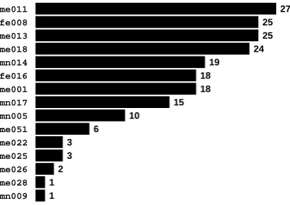
theBmrmeetings, i.e. those held by the group of 15 researchers working on the Meeting Recorder project at ICSI. Not all 15 persons participated in every meeting; each of the 29 meetings was at-tended by an average of 6.8 persons. The total number of conversationsidesin DATASETis 197.
The distribution of sides per participant is shown in Figure 1.
me011 fe008 me013 me018 mn014 fe016 me001 mn017 mn005 me051 me022 me025 me026 me028 mn009 1
1 2
3 3
6 10
15 18 18 19
24 25 25
[image:2.595.76.287.509.658.2]27
Figure 1: The number of sides in DATASET
con-tributed by each of its 15 participants.
Each meeting in the ICSI Meeting Corpus con-tains an interval of time (at the beginning or end of the meeting) marked asDigits, used for micro-phone calibration. This interval was excluded for
the current purposes, as it does not involve conver-sation. Each recording was left with between 22.8 and 74.5 minutes of data, with an average of 48.4 minutes.
3 Methodology
3.1 Chronograms
From each meetingCin DATASET, a
speech/non-speech chronogram (Chapple, 1949) was con-structed, designated by Q. Q is a matrix whose entries are one of{,}, or equivalently{0,1}, designating non-speech or speech respectively. Rows represent theKpersons participating in the meeting, while columns represent 100-ms time frames covering its temporal support. The
aver-ageQ in DATASET thus contained K = 7 rows
andT = 29K columns.
The cell in rowkand columnttof everyQwas
populated, by a value of or , by inspecting
the forced alignments to the manually transcribed speech attributed to the kth speaker of the cor-responding meeting. The transcriptions, attribu-tions, and alignments had been made available by ICSI in (Shriberg et al., 2004). A frame incre-ment of 100 ms was chosen as in (Laskowski et al., 2011b) and (Laskowski et al., 2011a); this is shorter than the average syllable duration, ensur-ing that no speech is missed, but longer than the frame step of the recognizer used by ICSI for the forced alignment. This makes the models devel-oped in the current work robust to imprecision in word start and end times.
3.2 Stochastic Turn-Taking Models
The models used in the current work are prob-abilistic generative models that, given a chrono-gram Q ∈ {,}K×T, provide the probability that its kth participant will speak during its tth frame. Participants are most commonly (Jaffe et al., 1967; Brady, 1969; Laskowski et al., 2011b) treated as conditionally independent (or “single-source” in the terminology of (Jaffe et al., 1967));
namely, the probability of speaking at frame t
for participantkis independent of what the other
K −1participants do at frame t, but it is condi-tioned on the jointK-participant history. The his-tory duration, in number of most-recent contigu-ous frames, is denoted henceforth byτ.
In multi-party conversation, the number K of
eliminate this complication, when constructing or
accessing the model describing the kth row of
chronogram Q, the remaining K −1 rows
(rep-resenting the kth participant’s interlocutors) are collapsed via an inclusive-OR operation, to pro-vide a single “all interlocutors” row. This results in a conditioning history of τ frames of the kth participant, and τ frames of context describing whether any of thekth participant’s interlocutors were speaking at instantt−τ (Laskowski et al., 2011b).
The above method yields a history duration which is independent of K, and lends itself
eas-ily to N-gram modeling. The elements of the
conditioning history are marshalled into a one-dimensional order, and counts are accumulated
as elsewhere for N-grams. This results in a
maximum-likelihood (ML) model pA(q|h) for a
sequence denotedA, withq ∈ {,}andh the
conditioning history. In (Laskowski et al., 2011b), such models were interpolated with lower-order (smaller-τ) models (Jelinek and Mercer, 1980), yielding smoothed models p˜A(q|h). In the
ab-sence of smoothing, as in the current work, the or-der of the elements of the(2×τ)-length history is unimportant, provided it is fixed.
3.3 Supervised Modeling
In supervised modeling, a modelAis constructed from one or more conversation sides attributed to the same speaker, and then that model is applied to a conversation sideBwhose speaker is unknown. In this case, a commonly used score between
gen-erative model A and sequence B is the average
negative log-likelihoodof the sequence given the
model, which is also known as the conditional
cross entropy:
H(pB(q|h)|p˜A(q|h))
= −X
h,q
pB(h, q) log ˜pA(q|h) , (1)
wherepB(h, q)are the ML joint probabilities
ob-served in sequenceB. Equation 1 is often normal-ized by subtracting theconditional entropy(Cover and Thomas, 1991),
H(pB(q|h))
= −X
h,q
pB(h, q) logpB(q|h) . (2)
yielding the conditional relative entropy or
con-ditional Kullback-Leibler divergence (Cover and
Thomas, 1991):
DKL(pB(q|h)kp˜A(q|h))
= X
h,q
pB(h, q) logpp˜B(q|h)
A(q|h) . (3)
For example, in the context of stochastic turn-taking models, Equation 1 was successfully used with zero-normalization of scores (Laskowski, 2014).
3.4 Unsupervised Modeling
In the unsupervised case, a score does not
nor-mally compare a sequence B to a model A, but
rather a sequence A to a sequence B (or, alter-nately, a model trained on sequenceAto a model trained on sequenceB). Because of this symme-try, it is desirable for the score itself to be symmet-ric; the conditional Kullback-Leibler divergence in Equation 3 does not exhibit this quality and, ad-ditionally, is unbounded. It is therefore custom-ary to compute the conditional Jensen-Shannon di-vergence (Lin, 1991), which for two equal-weight conditional probability modelspAandpBis given
by
DJS(pA(q|h)kpB(q|h))
≡ 12 DKL(pB(q|h)kp(q|h))
+ 1
2 DKL(pA(q|h)kp(q|h)) . (4)
Here, p(q|h) is the “joint-source” (ie. A andB) model; (El-Yaniv et al., 1997) showed that for models of conditional probability, its form is
p(q|h) = λA(h)·pA(q|h)
+ λB(h)·pB(q|h) , (5)
namely that it is the linear interpolation of the two single-source models, with weights given by their relative probabilities of the occurrence of the con-texth:
λA(h) = p pA(h)
A(h) +pB(h) (6)
λB(h) = p pB(h)
A(h) +pB(h) . (7)
The Jensen-Shannon distance, a score which is
both bounded and symmetric, is given by
dA,B ≡ p
Table 1: Leave-one-out (LOO) modified-KNN classification accuracies, using Jensen-Shannon distances
between STT models of individual conversation sides in DATASET. K specifies the maximal number
of neighbors;τ is the number of 100-ms frames of conditioning history. Each frame contains 2 bits of information: whether the modeled-side participant was speaking, and whether any of that participant’s interlocutors were speaking.
τ
K 1 2 3 4 5 6 7 8
1 0.37 0.44 0.56 0.54 0.47 0.37 0.18 0.09
3 0.36 0.53 0.51 0.55 0.48 0.37 0.16 0.09
5 0.40 0.53 0.59 0.58 0.49 0.34 0.15 0.07
7 0.40 0.54 0.59 0.57 0.49 0.33 0.16 0.07
9 0.41 0.54 0.57 0.57 0.50 0.33 0.13 0.07
11 0.43 0.55 0.59 0.57 0.52 0.33 0.15 0.08
13 0.43 0.54 0.60 0.57 0.54 0.34 0.15 0.09
15 0.45 0.54 0.60 0.58 0.54 0.35 0.18 0.10
17 0.45 0.54 0.59 0.59 0.55 0.36 0.20 0.13
19 0.45 0.55 0.60 0.58 0.54 0.38 0.21 0.13
25 0.44 0.53 0.57 0.57 0.53 0.38 0.21 0.13
3.5 Modified Nearest-Neighbor Classification A central goal of the current work is the determi-nation of whether two sequences, produced by the same person in different conversations, are more proximate than are two sequences produced by two different persons. One answer to this question can be provided by classifying sequences based on their proximity, of which the formalization is known as K-nearest neighbor classification (Fix and Hodges, 1951). The input to the algorithm is a symmetric, zero-diagonal distance matrix D, whose entries are pair-wise distances.
Here, a modified version of the algorithm is em-ployed. If the speakerg of the side being classi-fied is known to have produced onlyNg−1other
sides in the collection of sides under study, then
K is limited toNg−1for that classification trial.
The use of such side information may be perceived as unfair; however, the aim is diagnostic, and no effort has been made in the current work to nor-malize the distances inDfor local density differ-ences. In addition, it makes little sense to penal-ize an analysis for those trials whose speakers pro-duced no other sides in DATASET(cf. Section 2).
The results of such a diagnostic test can be use-fully compared to the outcome of random guess-ing under the same circumstances.
An alternative approach, consisting of applying clustering to the distance matrix, was also tried; the results yielded similar (albeit more difficult to
disentangle) results and are not presented due to space constraints.
3.6 Multidimensional Scaling
Finally, multidimensional scaling (MDS; cf. (Borg and Groenen, 2005) for example) was ap-plied in an attempt to embed models in a low-dimensional space and to facilitate visual analysis.
The experiments used the smacofSym()
func-tion (de Leeuw and Mair, 2009) implementafunc-tion in R.
4 Results
For a given τ ∈ [1,2,3, . . . ,8], each conversa-tion side qn of the N = 197 sides in DATASET
was used to train a side-specific maximum like-lihood (ML) modelθn. The distance between
ev-ery pair of models was then computed using Equa-tion 8, leading to a symmetric, zero-diagonal dis-tance matrixD∈R197×197
+ .
4.1 Diagnostic Classification
D was then used within the modified K-nearest
neighbor participant-identity classification frame-work described in Section 3.5. The achieved accu-racies are shown in Table 1.
As can be seen, the highest accuracies are ob-tained for τ ∈ [2,3,4,5] with K > 7, with an absolute maximum from among those
ex-plored of 60%, at τ = 3 and K = 15. This
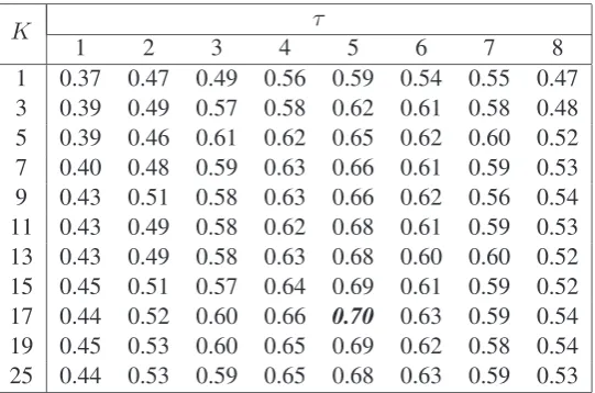
Table 2: LOO modified-KNN classification accuracies, using distances computed following multidimen-sional scaling (MDS) of the distances between STT models of individual conversation sides in DATASET,
to 5 dimensions. Compare to Table 1.
τ
K 1 2 3 4 5 6 7 8
1 0.37 0.47 0.49 0.56 0.59 0.54 0.55 0.47
3 0.39 0.49 0.57 0.58 0.62 0.61 0.58 0.48
5 0.39 0.46 0.61 0.62 0.65 0.62 0.60 0.52
7 0.40 0.48 0.59 0.63 0.66 0.61 0.59 0.53
9 0.43 0.51 0.58 0.63 0.66 0.62 0.56 0.54
11 0.43 0.49 0.58 0.62 0.68 0.61 0.59 0.53 13 0.43 0.49 0.58 0.63 0.68 0.60 0.60 0.52 15 0.45 0.51 0.57 0.64 0.69 0.61 0.59 0.52
17 0.44 0.52 0.60 0.66 0.70 0.63 0.59 0.54
19 0.45 0.53 0.60 0.65 0.69 0.62 0.58 0.54 25 0.44 0.53 0.59 0.65 0.68 0.63 0.59 0.53
achieved by random guessing with the DATASET
priors. This result corroborates the findings in (Laskowski, 2014), that participant identities can frequently be inferred from STT models; the dif-ference with (Laskowski, 2014) is that in the lat-ter work, models were trained on same-personsets of sides in a training portion of the data, rather than on individual sides, and that the asymmet-ric conditional cross entropy (Equation 2, with zero-normalization) was used rather than Jensen-Shannon divergence (Equation 4).
4.2 Diagnostic Classification after Scaling The computed pair-wise Jensen-Shannon dis-tances lie in a space of unknown effective dimen-sionality; the determination of that effective di-mensionality is one of the implicit aims of the cur-rent work. To this end, the distances were em-bedded in a fixed-dimensionality subspace, using multidimensional scaling (MDS) as described in Section 3.6. All 19306 pair-wise distances
com-prisingDwere then re-computed from the
MDS-derived positions, and the diagnostic experiment of Section 4.1 was repeated. The results for a 5-dimensional subspace are shown in Table 2.
As can be seen, relative to Table 1, MDS to 5 dimensions actually increases the attainable clas-sification accuracy, to 70% atτ = 5andK = 17. This suggests that there is considerable noise in the distance estimates, and that scaling effectively collapses some of that variability. The accuracy-maximizing number of dimensions, whose identi-fication is beyond the scope of the current work,
is expected to be specific to any particular data set. However, it is notable that for DATASET
this “elimination of unwanted variance” occurs for the higher-complexity (τ > 2) models; dis-tances computed using these are more likely to be noisy that those computed using simpler models, for fixed conversation-side durations. Since the
τ = 8context contains theτ = 5context, this sug-gests that the duration of the conversations studied here, between 22.8 and 74.5 minutes, may be in-sufficient to infer robust long-conditioning-history models.
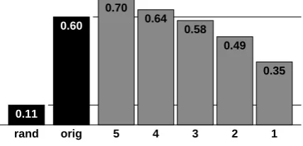
Similar experiments were performed after MDS scaling to each of{4,3,2,1}dimensions. The re-sults are not shown due to space constraints. A summary of the maximum achieved accuracy in each case is depicted in Figure 2.
The figure shows that with each reduction of di-mensionality of the embedding subspace, by one additional dimension, the maximum achievable accuracy falls by an increasing amount. Although for a one-dimensional subspace the accuracy of 35% is still considerably above chance (11%), it is already (just) less than halfway to the accuracy achieved without scaling (60%).
−1 −0.5 0 0.5 −1
−0.8 −0.6 −0.4 −0.2 0 0.2 0.4 0.6 0.8 1
DIM 1
DIM 2
me011 fe008 me013 me018 mn014 other
−1 −0.5 0 0.5 −1
−0.5 0 0.5 1
DIM 1
DIM 3
−1 −0.5 0 0.5 1
−1 −0.5 0 0.5 1
DIM 2
DIM 3
[image:6.595.84.518.59.224.2](a) dimensions 1 & 2 (b) dimensions 1 & 3 (c) dimensions 2 & 3
Figure 3: Positions of 197 models, each of one conversation side in DATASET, as inferred using a
Jensen-Shannon distance matrix and multidimensional scaling (MDS) to 3 dimensions. Sides produced by the five most frequently-occurring persons (cf. Section 2) are identified explicitly, together with ellipses representing projections of the corresponding 50% error ellipsoid.
rand orig 5 4 3 2 1 0.11
0.60 0.70
0.64 0.58
0.49
0.35
Figure 2: Maximum achieved LOO modified-KNN classification accuracies, using distances computed following MDS down to [5,4,3,2,1]
dimensions of the distances between STT mod-els of individual conversation sides in DATASET.
The accuracies are compared to the maximum ac-curacy achieved using unscaled distances (“orig”) and random guessing with actual LOO priors (“rand”).
with an independently measurable human trait or role trait. In that case, such traits could be used to index STT models, for both generation and recog-nition purposes in multi-party conversational set-tings.
4.3 Model Subspace Visualization
It is serendipitous that, for the data set under inves-tigation, three dimensions suffice to yield a good approximation of the accuracy achievable with-out scaling. A three-dimensional space is con-siderably easier to inspect visually, and to under-stand, than are higher-dimensional spaces. Fig-ure 3 shows the MDS-derived locations, two
di-mensions at a time. The 197 datapoints, repre-senting models of individual conversation sides, are seen to comprise a cloud with heterogenous, locally clumpy density. The determinant of the to-tal scatter matrix, given these inferred positions, is
2.74×10³.
The determinants of the between-class scatter matrix and the within-class scatter matrix, given the model positions shown in Figure 3, are3.29×
103 and 2.86 × 10³, respectively. It appears from these numbers that the variability between different-person sides is on average larger than the variability between same-person sides, which in turn suggests that people exhibit low variability — even across longitudinal spans of many months — relative to what differentiates them from others.
5 Discussion
5.1 Intra-Person Variability
It is relevant to try to determine whether the vari-ability observed among models of the same person are due to actual variability of behavior or to mea-surement error. One source of meamea-surement er-ror could be the relative duration of conversations, leading to unequally (under)trained models. Fig-ure 4 depicts the five most frequent participants in DATASET, at the same positions as in Figure 3(a),
with marker size indicative of the duration of ob-servation.
[image:6.595.75.289.313.416.2]par-−1 −0.5 0 0.5 −1
−0.8 −0.6 −0.4 −0.2 0 0.2 0.4 0.6 0.8 1
DIM 1
DIM 2
[image:7.595.311.524.60.279.2]me011 fe008 me013 me018 mn014
Figure 4: Replication of Figure 3(a) with marker size linearly proportional to the duration of con-versation from which each side is drawn. Sides for only the top five most frequent participants shown.
simonious — the resulting error ellipses (shown unchanged from Figure 3(a) in Figure 4) may be tighter, and thereby even more discriminative.
A second potential source of intra-person vari-ability may be not just the duration of observa-tion (i.e. the duraobserva-tion of conversaobserva-tion), but how talkative a person is during a specific conversa-tion. Although the models employed here make no mathematical distinction between speaking and not speaking, in multi-party turn-taking the av-erage participant speaks for only a minority of time, making speaking (versus not speaking) a dis-tinctively marked behavior. Figure 5 is like Fig-ure 4, but marker size is indicative of the amount of speech observed for each side.
Figure 5 shows that points lying in the bot-tom right of the figure represent low quantities of speech per side, globally. This appears to be true for individual speakers separately, particularly for the top three most frequent participants (and
me013 most markedly). Since the ellipses ap-pear cigar-shaped, fanning out from the bottom right, these observations suggest that when given the opportunity to speak a lot, participant models “move” to the upper left where they may be even further apart. They also suggest that a quantity en-coded in the plane of the first and second MDS dimensions (“DIM1” and “DIM2” in the figure) is the proportion of speech produced by each person,
−1 −0.5 0 0.5 −1
−0.8 −0.6 −0.4 −0.2 0 0.2 0.4 0.6 0.8 1
DIM 1
DIM 2
me011 fe008 me013 me018 mn014
Figure 5: Replication of Figure 3(a) with marker size linearly proportional to the amount of speech observed for each side. Sides for only the top five most frequent participants shown.
or their “talkativity”.
5.2 Inter-Person Variability
A source of established (Laskowski et al., 2008) variability in turn-taking models trained using the ICSI Meeting Corpus is the relative seniority of participants within a group. (Laskowski et al.,
2008) used the self-reported Education level.
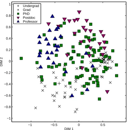
Figure 6 retains the topology shown in Figure 3(a), but markers represent the educational level of in-dividual participants in DATASET. It can be seen
that students (Undergrad and Grad) occupy
exclusively the lower half in the diagram, while
Postdoc andProfessor are found predomi-nantly in the upper half, but in separate clusters. Persons of typePhDexhibit no such leanings.
Figure 6 suggests that education level is indeed discriminated by the STT-model topology inferred via MDS. (Laskowski et al., 2008) observed that despite the fact that persons of typeProfessor
[image:7.595.78.288.60.278.2]terminate talk in overlap.
−1 −0.5 0 0.5 −1
−0.8 −0.6 −0.4 −0.2 0 0.2 0.4 0.6 0.8 1
DIM 1
DIM 2
[image:8.595.76.289.87.304.2]Undergrad Grad PhD Postdoc Professor
Figure 6: Replication of Figure 3(a) with marker shape denoting the self-reported education level of each side.
It should be noted that, unlike the measure-ment of intra-person variability, the measuremeasure-ment of inter-person variability is likely a function of the size of the group of people studied. As de-scribed in Section 2, the group considered here consists of 15 individuals, some of which partic-ipated in only a handful of conversations. For larger groups, it can be expected that — if models represent interaction styles — inter-person vari-ability under a fixed model order and a fixed ob-servation duration will decrease, since nothing a priori prevents multiple individuals from interact-ing usinteract-ing the same or similar-enough style. Since intra-person variability is independent of the num-ber of other persons considered, it is expected to remain constant under group resizing. The ratio of the inter-person variability to the intra-person vari-ability is therefore likely to decrease with increas-ingly larger group sizes, when the model complex-ity and observational duration remain constant. 5.3 Training Speaker-Independent Models That within-person SST-model variability can be smaller than between-person variability, as discov-ered in the dataset used in the current study, has important consequences for training broad STT models, intended to be applicable to a wide variety of domains and conversational interaction styles. The results presented indicate that including more
training data, without careful consideration of its interaction-style content, may bias the model to-wards the styles present in the training data and therefore away from the styles in test data — since they can be so different. In this sense, the re-sults corroborate earlier, similar findings for do-main and topic variability in language modeling within automatic speech recognition.
5.4 Potential Impact and Applications
Over and above the immediate recommendations for the training of STT models, the results ob-tained in the current study may have several con-sequences for at least three research areas.
An understanding of the contexts in which par-ticipants to conversation choose to vocalize can usefully inform the construction of speaker di-arization systems. Current state-of-the-art diariza-tion technology, as used in the transcripdiariza-tion of far-field recordings of multi-party meetings, over-segments the temporal support of the recorded track and then performs agglomerative hierarchi-cal clustering using spectral or voice-print similar-ity. The prior knowledge used in these systems consists of minimal duration constraints on inter-vals of single-party talk, as well as the assump-tion that each instant is associated with exactly one participant speaking. The detection of overlap (or of simultaneous vocalization by more than one speaker), where performed, is generally treated as a post-processing step. Information regarding con-sistent, participant-specific tendencies in the tem-poral deployment of talk — the subject of the cur-rent study — do not curcur-rently feature in any way in the assumptions or priors of today’s diarization systems.
self-consistent and differentiable style, which is syn-tonic with its designed conversational role.
Finally, the results in this study have bearing on the design of diagnostic tools for social psychol-ogy, the domain for which STT models were orig-inally invented (Chapple, 1949; Jaffe et al., 1967). (Chapple, 1949) was concerned with the measure-ment of conversational traits correlated with work performance, whereas (Jaffe et al., 1967) treated clinical settings. A considerable amount of re-search in this area had been conducted in the 1970s and 1980s, primarily in the detection of traits or conditions. However, the models were first-order
Markovian (corresponding to τ = 1 in the
cur-rent work) and often relying on analysis frames as small as 20 ms. The findings presented here indicate that useful speaker-discriminating infor-mation is contained as far back as 500 ms (with frames of 100 ms andτ = 5, cf. Subsection 4.2), even when models are trained on single conver-sations which are as short as 22 minutes long. The obtained results may warrant a re-opening of earlier investigations into diagnostic tools for the health industry.
6 Conclusions
That people exhibit a degree of consistency in their conversational behavior agrees with com-mon sense, and should not be particularly surpris-ing. A number of earlier works have success-fully correlated identity with turn-taking prefer-ences (Jurafsky et al., 2009; Grothendieck et al., 2011). What the analyses in the current work show — and which is surprising — is that this consistency is present even in the very shallow representation implicit in the so-called stochastic turn-taking models. In this representation, words, boundaries, durations, and prosody are markedly absent; only the frame-level occurrence of party-attributed speech activity is captured, and a defini-tion of “turn” is neither needed nor used. Specifi-cally, results indicate that, for conversations whose duration is 40-minutes on average, longitudinally speaker-discriminative models can be learned for a conditioning history which is only 10 bits long: whether the modeled speaker, andanyof their in-terlocutors, were speaking in each of the 5 most recent 100-ms frames. The current study has shown that under these conditions, for groups of 15 people like the ICSI Bmr group, the inferred models exhibit greater between-person
variabil-ity than within-person variabilvariabil-ity. The conver-stants under study appear to have behaved self-consistently, across disparate longitudinal obser-vations, in terms of their turn-taking preferences.
The current experiments also demonstrated that
a conversation-side embedding in three
dimen-sions approximately recovers the Jensen-Shannon distances between 10-bit-context STT models. In this embedding, between-person variability was shown to be smaller for longer conversations, im-plying that over time people can be observed to converge on interaction styles which are even more self-consistent. Although it is premature to unambiguously ascribe meaning to each of the
three dimensions obtained using the ICSI Bmr
data, jointly they appear to encode: (1) the pro-portion of conversation-time spent talking; (2) the inclination to initiate and terminate overlap with others; and (3) role-specific behaviors exhibited by members of a hierarchy (with — in the current work — positions within that hierarchy closely correlated with self-reported education level).
The presented work suggests the possibility of inference of speaker-characterizing conversational interaction styles, as well as the indexing of such interaction styles by points in an embedding space consisting of only a few continuous dimensions. It has immediate bearing on the training of inten-tionally broad, speaker-independent STT models. Finally, the work has the potential to usefully im-pact the design of speaker diarization algorithms for multi-human conversation settings, of human-like conversational dialogue systems, and of diag-nostic software for the health industry.
7 Acknowledgments
This work was funded in part by the Riksbankens
Jubileumsfond (RJ) project Samtalets Prosodi.
References
I. Borg and P. Groenen. 2005. Modern Multidimen-sional Scaling: Theory and Applications. Springer.
P. Brady. 1969. A model for generating on-off speech patterns in two-way conversation. The Bell System Technical Manual, 48(9):2445–2472.
E. Chapple. 1949. The Interaction Chronograph: Its evolution and present application. Personnel, 25(4):295–307.
T. Cover and J. Thomas, 1991. Elements of Informa-tion Theory, chapter Entropy, Relative Entropy and Mutual Information (Chapter 2), pages 12–49. John Wiley & Sons, Inc.
J. de Leeuw and P. Mair. 2009. Multidimensional scal-ing usscal-ing majorization: SMACOF in R. Journal of Statistical Software, 31(3):1–30.
R. El-Yaniv, S. Fine, and N. Tishby. 1997. Agnos-tic classification of Markovian sequences. InProc. Advances in Neural Information Processing Systems (NIPS) 10, pages 465–471, Denver CO, USA.
E. Fix and J. Hodges. 1951. Discriminatory analysis, nonparametric discrimination: Consistency proper-ties. Technical report, USAF School of Aviation Medicine, Randolph Field TX, USA.
J. Grothendieck, A. Gorin, and N. Borges. 2011. So-cial correlates of turn-taking style. Comput. Speech Lang., 25(4):789–801, October.
Jr. J. Dabbs and R. Ruback. 1987. Dimensions of group process: Amount and structure of vocal inter-action. Advances in Experimental Social Psychol-ogy, 20:123–169.
J. Jaffe, S. Feldstein, and L. Cassotta. 1967. Marko-vian models of dialogic time patterns. Nature, 216:93–94.
A. Janin, D. Baron, J. Edwards, D. Ellis, D. Gelbart, N. Morgan, B. Peskin, T. Pfau, E. Shriberg, A. Stol-cke, and C. Wooters. 2003. The ICSI Meeting Corpus. InProc. 28th IEEE International Confer-ence on Acoustics, Speech, and Signal Processing (ICASSP), pages 364–367, Hong Kong, China.
F. Jelinek and R. Mercer. 1980. Interpolated estima-tion of Markov source parameters from sparse data. InProc. Workshop on Pattern Recognition in Prac-tice, Amsterdam, The Netherlands.
D. Jurafsky, R. Ranganath, and D. McFarland. 2009. Extracting social meaning: Identifying interactional style in spoken conversation. InProc. Annual Con-ference of the North American Chapter of the Asso-ciation for Computational Linguistics, pages 638– 646, Boulder CO, USA.
K. Laskowski, M. Ostendorf, and T. Schultz. 2008. Modeling vocal interaction for text-independent par-ticipant characterization in multi-party conversation. In Proc. 9th ISCA/ACL SIGdial Workshop on Dis-course and Dialogue, Columbus OH, USA. K. Laskowski, J. Edlund, and M. Heldner. 2011a.
In-cremental learning and forgetting in stochastic turn-taking models. InProc. 12th Annual Conference of the International Speech Communication Associa-tion (INTERSPEECH), pages 2065–2068, Firenze, Italy.
K. Laskowski, J. Edlund, and M. Heldner. 2011b. A single-port non-parametric model of turn-taking in multi-party conversation. InProc. 36th IEEE Inter-national Conference on Acoustics, Speech, and Sig-nal Processing (ICASSP), pages 5600–5603, Praha, Czech Republic.
K. Laskowski. 2010. Modeling norms of turn-taking in multi-party conversation. In Proc. 48th Annual Meeting of the Association for Computational Lin-guistics (ACL), pages 999–1008, Uppsala, Sweden. K. Laskowski. 2012. Exploiting loudness dynamics in
stochastic models of turn-taking. InProc. 4th IEEE Workshop on Spoken Language Technology (SLT), pages 79–84, Miami FL, USA.
K. Laskowski. 2014. On the conversant-specificity of stochastic turn-taking models. InProc. 15th Annual Conference of the International Speech Communi-cation Association (INTERSPEECH), pages 2026– 2030, Singapore.
J. Lin. 1991. Divergence measrures based on the Shannon entropy. IEEE Trans. Information Theory, 37(1):145–151.
E. Shriberg, R. Dhillon, S. Bhagat, J. Ang, and H. Car-vey. 2004. The ICSI Meeting Recorder Dialog Act (MRDA) Corpus. In Proc. 5th ISCA/ACL SIGdial Workshop on Discourse and Dialogue, pages 97– 100, Cambridge MA, USA.