Structure Sharing with Binary Trees

Structure Sharing with Binary Trees

Lauri Karttunen SRI International, CSLI Stanford

Martin Kay Xerox PARC, CSU Stanford

Many current interfaces for natural language

represent syntactic and semantic information in the

form of directed graphs where attributes correspond

to vectors and values to nodes. There is a simple

correspondence between such graphs and the matrix

notation linguists traditionally use for feature sets.

.

' n " < ' a ' " "

sg 3rd

b.

Figure I

The standard operation for working with such graphs

is unification. The unification operation succedes only

on a pair of compatible graphs, and its result is a

graph containing the information in both

contributors. When a parser applies a syntactic rule, it unifies selected features of input constituents to

check constraints and to budd a representat=on for the output constituent.

Problem: proliferation of copies

When words are combined to form phrases,

unification is not applied to lexlcat representations directly because it would result in the lexicon being

changed. When a word is encountered in a text, a

copy is made of its entry, and unification is applied to

the copied graph, not the original one. In fact,

unification in a typical parser is always preceded by a

copying operation. Because of nondeterminism in

parsing, it is, in general, necessary to preserve every

representation that gets built. The same graph may

be needed again when the parser comes back to

pursue some yet unexplored option. Our experience

suggests that the amount of computational effort

that goes into producing these copies is much greater

than the cost of unification itself. It accounts for a

significant amount of the total parsing time.

In a sense, most of the copying effort is wasted. Unifications that fail typically fail for a simple reason.

If it were known in advance what aspects of structures are relevant in a particular case, some effort could be

saved by first considering only the crucial features of

the input.

Solution: structure sharing

This paper lays out one strategy that has turned out to

be very useful in eliminating much of the wasted

effort. Our version of the basic idea is due to Martin Kay. It has been implemented in slightly different

ways by Kay in Interlisp-O and by Lauri Karttunen in

Zeta Lisp. The basic idea is to minimize copying by

allowing graphs share common parts of their

structure.

This version of structure sharing is based on four

• Binary trees as a storage device for feature

graphs

• "Lazy" copying

• Relative indexing of nodes in the tree

• Strategy for keeping storage trees as balanced

as possible

Binary trees

Our structure-sharing scheme depends on

represented feature sets as binary trees. A tree

consists of cells that have a content field and t w o

pointers which, if not empty, point to a left and a

right cell respectively. For example, the content of the

feature set and the corresponding directed graph in

Figure 1 can be distributed over the cells of a binary

tree in the following way.

Figure 2

The index of the top node is 1; the two cells below have indices 2 and 3. In general, a node whose index

is n may be the parent of ceils indexed 2n and 2n + 1.

Each cell contains either an atomic value or a set of

pairs that associate attribute names with indices of

cells where their value is stored. The assignment of

vaiues to storage cells is arbitrary; =t doesn't matter

which cell stores which value. Here, cell 1 conta,ns the

information that the value of the at"tribute cat is found in ceil 2 and that of agr in cell 3. This is a slight

simplification. As we shall shortly see, when the value in a cell involves a reference to another cell, that

reference is encoded as a relative index.

The method of locating the cell that corresponds to a

given index takes advantage of the fact that the tree branches in a binary fashion. The path to a node can

be read o f f from the binary representation of its index

by starting after the first 1 in this number and taking 0

to be a signal for a left turn and 1 as a mark for a right

turn. For example, starting at node 1, node S is

reached by first going down a left branch and then a

right branch. This sequence of turns corresponds to

the digits 01. Prefixed with 1, this is the same as the

binary representation of 5, namely 101. The same

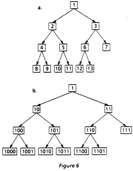
holds for all indices. Thus the path to node 9 (binary 1001) would be LEFT-LEFT-RIGHT as signalled by the

last three digits following the initial 1 in the binary

numeral (see Figure 6).

Lazy copying

The most important advantage that the scheme

minimizes the amount of copying that has to be done.

In general, when a graph is copied, we duplicate only

The operation that replaces copying in this scheme

starts by duplicating the topmost node of the tree

that contains it. The rest of the structure remains the

same. It is Other nodes are modified only ~f and when

destructive changes are about to happen. For

example, assume that we need another copy of the

graph stored in the tree in Figure 2. This can be

obtained by producing a tree which has a different

root node, but shares the rest of the structure with its original. In order to keep track of which tree actually

owns a given node, each node tames a numeral tag

that indicates its parentage. The relationship

between the original tree (generation 0) and its copy

(generation 1) is illustrated in Figure 3 where the

generation is separated from the index of a node by a

colon.

1:0 1:1

person 4 2:0 I n p l 3:0 _{number S}

4:0 S:O

If the node that we want to copy is not the topmost

node of a tree, we need to duplicate the nodes along

the branch leading to it.

When a tree headed by the copied node has to be

changed, we use the generation tags to minimize the

creation of new structure. In general, all and only the

nodes on the branch that lead to the site of a

destructive change or addition need to belong to the

same generation as the top node of the tree. The rest

of the structure can consist of old nodes. For example,

suppose we add a new feature, say [gender: femJ to

the value of agr in Figure 3 to yield the feature set in

Figure 4.

p

gender: fern

Figure 4

Furthermore, suppose that we want the change to

affect only the copy but not the original feature set.

In terms of the trees that we have constructed for the example in Figure 3, this involves adding one new cell

to the copied structure to hold the value fem, and

changing the content of cell 3 by adding the new

feature to it.

The modified copy and its relation to the original is

shown in Figure S. Note that one half of the structure

is shared. The copy contains only three new nodes.

2 : 0 ~ 4

/

~

/ " ~ gender 6

4:0,1~"]

S:oF'~

f

6:1 ~m'--~,

Figure 5

From the point of view of a process that only needs to find or print out the value of particular features, it

makes no difference that the nodes containing the

values belong to several ,trees as long as there is no

confusion about the structure.

Relative addressing

Accessing an arbitrary cell in a binary tree consumes

time in proportion to the logarithm of the size of the

structure, assuming that cells are reached by starting at the top node and using the index of the target

node as an address. Another method is to use relative

addressing. Relative addresses encode the shortest

path between two nodes in the tree regardless of

where they are are. For example, if we are at node 9

in Figure 6.a below and need to reach node 11, it is

easy to see that it is not necessary to go all the way up

to node 1 and then partially retrace the same path in

looking up node 11. instead, one can stop going

upward at the lowest common ancestor, node 2., of

nodes 9 and 11 and go down from there.

a.

Figure 6

up, then down as if going to node 7". In general,

relative addresses are of the form <up,down > where

< u p > is the number of links to the lowest common

ancestor of the origin and < d o w n > is the relative

index of the target node with respect to it.

Sometimes we can just go up or down on the same

branch; for example, the relative address of cell 10

seen from node 2 is simply 0,6; the path from 8 or 9 to

4is 1,1.

As one might expect, it is easy to see these

relationships if we think of node indices in their

binary representation (see Figure 6.b). The lowest

common ancestor 2 (binary 10) is designated by the

longest common initial substring of 9 (binary 1001)

and 11 (binary 1011). The relative index of 11, with respect to, 7 (binary 111), is the rest of its index with 1

prefixed to the front.

In terms of number of links traversed, relative

addresses have no statistical advantage over the

simpler method of always starting from the top. However, they have one important property that is

essential for our purposes: relative addresses remain

valid even when trees are embedded ~n other trees; absolute indices would have to be recalculated.

Figure 7 is a recoding of Figure S using relative addresses.

2:0 ~ 3.01 ~ o ~ , ~ 1 ~ I ~ : l l person1,4

/ \

I

I number 1,s

4:01 ira I 5:01 sg I 6:1

Figure 7

K e e p i n g t r e e s b a l a n c e d

When two feature matrices are unified, the binary

trees corresponding to them have to be combined to form a single tree. New attributes are added to some

of the nodes; other nodes become "pointer nodes,"

i.e., their only content is the relative address of some

other node where the real content is stored. As long

as we keep adding nodes to one tree, it is a simple

matter to keep the tree maximally balanced. At any

given time, only the growing fringe of the tree can be

incompletely filled. When two trees need to be

combined, it would, of course, be possible to add all

the cells from one tree in a balanced fashion to the

other one but that would defeat the very purpose of

using binary trees because it would mean having to

copy almost all of the structure. The only alternative

is to embed one of the trees in the other one. The

resulting tree will not be a balanced one; some of the

branches are much longer than others. Consequently,

the average time needed to look up a value ~s bound

to be worse than in a balanced tree.

For example, suppose that we want to unify a copy of

the feature set in Figure lb, represented as in Figure 2

but with relative addressing, with a copy of the

feature set in Figure 8.

a. agr: [gender: fem]]

l:01agr0,2 J

gender

2:ol

1,31

3:o

Figure 8

a. [-cat: np

I person: 3rd I I Lagr: I-number: sg-~

Lgender : fem~J

I cat0,2 l b. 1"1 aqr0,3

Z . 0 [ ~ ~ ~ ~ ~ ~ n 1,4

• ~1_:.~ I number 1,5

1:11 agrO,2 I

2:11 --> 2,1 I

3:0

Although the feature set in Figure 9.a is the same as

the one represented by the right half of Figure 7, the

structure in Figure 9.b is more complicated because it

is derived by unifying copies of t w o separate trees, not by simply adding more features to a tree, as in

Figure 7. In 9 b , a copy of 8.b has been embedded as

node 6 of the host tree. The original indices of both

trees remain unchanged. Because all the addresses are relative; no harm comes from the fact that indices

in the embedded tree no longer correspond to the

true location of the nodes. Absolute indices are not

used as addresses because they change when a tree is

embedded. The symbol - > in node 2 of the lower tree

indicates that the original content of this

node--<jender 1,3~has been replaced by the address

of the cell that it was unified with, namely cell 3 in the host tree.

In the case at hand, it matters very little which of the

t w o trees becomes the host for the other. The

resulting tree is about as much out of balance either

way. However, when a sequence of unifications is

~erformed, differences can be very significant. For

example, if A, B, and C are unified with one another, ~t

can make a great deal of difference, which of the t w o alternative shapes in Figure 10 is produced as the final result.

A A

.., ¢ ~

~

,&

Figure 10

When a choice has to be made as to which of the t w o

• ,rees to embed in the other, it is important to

minimize the length of the longest path in the

resulting tree. To do this at all efficiently requires addtitional infornation to be stored with each node. According to one simple scheme, this is simply the

length of the shortest path from the node down to a

node with a free left or right pointer. Using this, it is a

simple matter to find the shallowest place in a tree at

which to embed another one. If the length of the

longer path is also stored, it is also easy to determine

which choice of host will give rise to the shallowest combined tree.

Another problem which needs careful attention

concerns generation markers. If a pair of trees to be

unified have independent histories, their generation

markers will presumably be incommensurable and

those of an embedded tree will therfore not be valide in the host. Various solutions are possible for this

problem. The most straightforward is relate the histories of all trees at least to the extent of drawing

generation markers from a global pool. In Lisp, for

example, the simplest thing is to let them be CONS cells.

C o n c l u s i o n

We will conclude by comparing our method of

structure sharing with two others that we know of: R.

Cohen's immutable arrays and the idea discussed in

Fernando Pereira's paper at this meeting. The three

alternatives involve different trade-offs along the

space/time continuum. The choice between them wdl

depend on the particular application they are intended for. No statistics on parsing are avadable yet

but we hope to have some in the final version.

A c k n o w l e d g e m e n t s

This research, made possible in part by a gift from the

Systems Development Foundation, was also

supported by the Defense Advanced Research Projects

Agency under Contracts N00039-80- C-0575 and

N00039-84-C-0524 with the Naval Electronic Systems Command. The views and conclusions contained in

this document are those of the author and should not

be interpreted as representative of the official policies, either expressed or implied, of the Defense

Advanced Research Projects Agency, or the United