Fast and Robust Neural Network Joint Models for Statistical Machine Translation

Fast and Robust Neural Network Joint Models for Statistical Machine

Translation

Jacob Devlin, Rabih Zbib, Zhongqiang Huang, Thomas Lamar, Richard Schwartz,andJohn Makhoul

Raytheon BBN Technologies, 10 Moulton St, Cambridge, MA 02138, USA {jdevlin,rzbib,zhuang,tlamar,schwartz,makhoul}@bbn.com

Abstract

Recent work has shown success in us-ing neural network language models (NNLMs) as features in MT systems. Here, we present a novel formulation for a neural network joint model (NNJM), which augments the NNLM with a source context window. Our model is purely lexi-calized and can be integrated into any MT decoder. We also present several varia-tions of the NNJM which provide signif-icant additive improvements.

Although the model is quite simple, it yields strong empirical results. On the NIST OpenMT12 Arabic-English condi-tion, the NNJM features produce a gain of +3.0 BLEU on top of a powerful, feature-rich baseline which already includes a target-only NNLM. The NNJM features also produce a gain of +6.3 BLEU on top of a simpler baseline equivalent to Chi-ang’s (2007) original Hiero implementa-tion.

Additionally, we describe two novel tech-niques for overcoming the historically high cost of using NNLM-style models in MT decoding. These techniques speed up NNJM computation by a factor of 10,000x, making the model as fast as a standard back-off LM.

This work was supported by DARPA/I2O Contract No. HR0011-12-C-0014 under the BOLT program (Approved for Public Release, Distribution Unlimited). The views, opin-ions, and/or findings contained in this article are those of the author and should not be interpreted as representing the of-ficial views or policies, either expressed or implied, of the Defense Advanced Research Projects Agency or the Depart-ment of Defense.

1 Introduction

In recent years, neural network models have be-come increasingly popular in NLP. Initially, these models were primarily used to createn-gram neu-ral network language models (NNLMs) for speech recognition and machine translation (Bengio et al., 2003; Schwenk, 2010). They have since been ex-tended to translation modeling, parsing, and many other NLP tasks.

In this paper we use a basic neural network ar-chitecture and a lexicalized probability model to create a powerful MT decoding feature. Specifi-cally, we introduce a novel formulation for a neu-ral network joint model (NNJM), which augments ann-gram target language model with anm-word source window. Unlike previous approaches to joint modeling (Le et al., 2012), our feature can be easily integrated into any statistical machine trans-lation (SMT) decoder, which leads to substantially larger improvements than k-best rescoring only. Additionally, we present several variations of this model which provide significant additive BLEU gains.

We also present a novel technique for training the neural network to be self-normalized, which avoids the costly step of posteriorizing over the entire vocabulary in decoding. When used in con-junction with apre-computed hidden layer, these techniques speed up NNJM computation by a fac-tor of 10,000x, with only a small reduction on MT accuracy.

Although our model is quite simple, we obtain strong empirical results. We show primary results on the NIST OpenMT12 Arabic-English condi-tion. The NNJM features produce an improvement of +3.0 BLEU on top of a baseline that is already better than the 1st place MT12 result and includes

a powerful NNLM. Additionally, on top of a sim-pler decoder equivalent to Chiang’s (2007) origi-nal Hiero implementation, our NNJM features are able to produce an improvement of +6.3 BLEU – as much as all of the other features in our strong baseline system combined.

We also show strong improvements on the NIST OpenMT12 Chinese-English task, as well as the DARPA BOLT (Broad Operational Language Translation) Arabic-English and Chinese-English conditions.

2 Neural Network Joint Model (NNJM) Formally, our model approximates the probability of target hypothesisT conditioned on source sen-tenceS. We follow the standardn-gram LM de-composition of the target, where each target word

ti is conditioned on the previous n − 1 target

words. To make this ajointmodel, we also condi-tion on source context vectorSi:

P(T|S) ≈ Π|_iT₌₁|P(ti|ti−1,· · ·, ti−n+1,Si)

Intuitively, we want to defineSias the window that is most relevant toti. To do this, we first say

that each target word ti isaffiliated with exactly

one source word at indexai.Siis then them-word

source window centered atai: Si = s_ai−m−1

2 ,· · · , sai,· · · , sai+m2−1

This notion of affiliation is derived from the word alignment, but unlike word alignment, each target word must be affiliated with exactly one non-NULL source word. The affiliation heuristic is very simple:

(1) If ti aligns to exactly one source word,ai is

the index of the word it aligns to.

(2) Ifti align to multiple source words,ai is the

index of the aligned word in the middle.1

(3) If ti is unaligned, we inherit its affiliation

from the closest aligned word, with prefer-ence given to the right.2

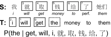
An example of the NNJM context model for a Chinese-English parallel sentence is given in Fig-ure 1.

For all of our experiments we use n = 4 and

m = 11. It is clear that this model is effectively an(n+m)-gram LM, and a 15-gram LM would be

1_{We arbitrarily round down.}

2_{We have found that the affiliation heuristic is robust to}

small differences, such as left vs. right preference.

far too sparse for standard probability models such as Kneser-Ney back-off (Kneser and Ney, 1995) or Maximum Entropy (Rosenfeld, 1996). Fortu-nately, neural network language models are able to elegantly scale up and take advantage of arbi-trarily large context sizes.

2.1 Neural Network Architecture

Our neural network architecture is almost identi-cal to the original feed-forward NNLM architec-ture described in Bengio et al. (2003).

The input vector is a 14-word context vector (3 target words, 11 source words), where each word is mapped to a 192-dimensional vector us-ing a shared mappus-ing layer. We use two 512-dimensional hidden layers with tanh activation functions. The output layer is a softmax over the entire output vocabulary.

The input vocabulary contains 16,000 source words and 16,000 target words, while the out-put vocabulary contains 32,000 target words. The vocabulary is selected by frequency-sorting the words in the parallel training data. Out-of-vocabulary words are mapped to their POS tag (or

OOV, if POS is not available), and in this case

P(P OSi|ti−1,· · ·) is used directly without fur-ther normalization. Out-of-bounds words are rep-resented with special tokens <src>, </src>,

<trg>,</trg>.

We chose these values for the hidden layer size, vocabulary size, and source window size because they seemed to work best on our data sets – larger sizes did not improve results, while smaller sizes degraded results. Empirical comparisons are given in Section 6.5.

2.2 Neural Network Training

The training procedure is identical to that of an NNLM, except that the parallel corpus is used instead of a monolingual corpus. Formally, we seek to maximize the log-likelihood of the train-ing data:

L=X

i

log(P(xi))

wherexiis the training sample, with one sample

Figure 1: Context vector for target word “the”, using a 3-word target history and a 5-word source window (i.e.,n= 4andm= 5). Here, “the” inherits its affiliation from “money” because this is the first aligned word to its right. The number in each box denotes the index of the word in the context vector. This indexing must be consistent across samples, but the absolute ordering does not affect results.

128.3 _{At every epoch, which we define as 20,000}

minibatches, the likelihood of a validation set is computed. If this likelihood is worse than the pre-vious epoch, the learning rate is multiplied by 0.5. The training is run for 40 epochs. The training data ranges from 10-30M words, depending on the condition. We perform a basic weight update with no L2 regularization or momentum. However, we have found it beneficial to clip each weight update to the range of [-0.1, 0.1], to prevent the training from entering degenerate search spaces (Pascanu et al., 2012).

Training is performed on a single Tesla K10 GPU, with each epoch (128*20k = 2.6M samples) taking roughly 1100 seconds to run, resulting in a total training time of ∼12 hours. Decoding is performed on a CPU.

2.3 Self-Normalized Neural Network

The computational cost of NNLMs is a significant issue in decoding, and this cost is dominated by the output softmax over the entire target vocabu-lary. Even class-based approaches such as Le et al. (2012) require a 2-20k shortlist vocabulary, and are therefore still quite costly.

Here, our goal is to be able to use a fairly large vocabulary without word classes, and to sim-ply avoid computing the entire output layer at de-code time.4 _{To do this, we present the novel}

technique ofself-normalization, where the output layer scores are close to being probabilities with-out explicitly performing a softmax.

Formally, we define the standard softmax log

3_{We donotdivide the gradient by the minibatch size. For}

those who do, this is equivalent to using an initial learning rate of10−3_∗128≈10−1_.

4_{We are not concerned with speeding up training time, as}

we already find GPU training time to be adequate.

likelihood as:

log(P(x)) = log eUr(x)

Z(x)

!

= Ur(x)−log(Z(x)) Z(x) = Σ_r|V0₌₁| eUr0(x)

wherexis the sample,U is the raw output layer scores,ris the output layer row corresponding to the observed target word, andZ(x)is the softmax normalizer.

If we could guarantee that log(Z(x)) were al-ways equal to 0 (i.e., Z(x) = 1) then at decode time we would only have to compute rowrof the output layer instead of the whole matrix. While we cannot train a neural network with this guaran-tee, we can explicitly encouragethe log-softmax normalizer to be as close to 0 as possible by aug-menting our training objective function:

L = X

i

log(P(xi))−α(log(Z(xi))−0)2

= X

i

log(P(xi))−αlog2(Z(xi))

In this case, the output layer bias weights are initialized to log(1/|V|), so that the initial net-work is self-normalized. At decode time, we sim-ply use Ur(x) as the feature score, rather than

log(P(x)). For our NNJM architecture, self-normalization increases the lookup speed during decoding by a factor of∼15x.

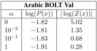
Table 1 shows the neural network training re-sults with various values of the free parameter

α. In all subsequent MT experiments, we use

α= 10−1_.

Arabic BOLT Val α log(P(x)) |log(Z(x))|

0 −1.82 5.02 10−2 _{−1.81 1.35} 10−1 _{−1.83 0.68} 1 −1.91 0.28

Table 1: Comparison of neural network likelihood for various α values. log(P(x)) is the average log-likelihood on a held-out set. |log(Z(x))|is the mean error in log-likelihood when usingUr(x)

directly instead of the true softmax probability log(P(x)). Note thatα = 0is equivalent to the standard neural network objective function.

is no mechanism to control the degree of self-normalization. By contrast, our α parameter al-lows us to carefully choose the optimal trade-off between neural network accuracy and mean self-normalization error. In future work, we will thor-oughly compare self-normalization vs. NCE.

2.4 Pre-Computing the Hidden Layer

Although self-normalization significantly im-proves the speed of NNJM lookups, the model is still several orders of magnitude slower than a back-off LM. Here, we present a “trick” for pre-computing the first hidden layer, which further in-creases the speed of NNJM lookups by a factor of 1,000x.

Note that this technique only results in a signif-icant speedup for self-normalized, feed-forward, NNLM-style networks withonehidden layer. We demonstrate in Section 6.6 that using one hidden layer instead of two has minimal effect on BLEU. For the neural network described in Section 2.1, computing the first hidden layer requires mul-tiplying a 2689-dimensional input vector5 _with

a 2689 ×512 dimensional hidden layer matrix. However, note that there are only 3 possible posi-tions for each target word, and 11 for each source word. Therefore, for every word in the vocabu-lary, and for each position, we can pre-compute the dot product between the word embedding and the first hidden layer. These are computed offline and stored in a lookup table, which is<500MB in size.

Computing the first hidden layer now only re-quires 15 scalar additions for each of the 512 hidden rows – one for each word in the input

5_{2689 = 14 words×192 dimensions + 1 bias}

vector, plus the bias. This can be reduced to just 5 scalar additions by pre-summing each 11-word source window when starting a test sen-tence. If our neural network has only one hid-den layer and is self-normalized, the only remain-ing computation is 512 calls totanh()and a sin-gle 513-dimensional dot product for the final out-put score.6 _{Thus, only ∼3500 arithmetic}

opera-tions are required per n-gram lookup, compared to∼2.8M for self-normalized NNJM without pre-computation, and∼35M for the standard NNJM.7

Neural Network Speed

Condition lookups/sec sec/word

Standard 110 10.9

+ Self-Norm 1500 0.8

+ Pre-Computation 1,430,000 0.0008 Table 2: Speed of the neural network computa-tion on a single CPU thread. “lookups/sec” is the number of uniquen-gram probabilities that can be computed per second. “sec/word” is the amortized cost of unique NNJM lookups in decoding, per source word.

Table 2 shows the speed of self-normalization and pre-computation for the NNJM. The decoding cost is based on a measurement of∼1200 unique NNJM lookups per source word for our Arabic-English system.8

By combining self-normalization and pre-computation, we can achieve a speed of 1.4M lookups/second, which is on par with fast back-off LM implementations (Tanaka et al., 2013). We demonstrate in Section 6.6 that using the self-normalized/pre-computed NNJM results in only a very small BLEU degradation compared to the standard NNJM.

3 Decoding with the NNJM

Because our NNJM is fundamentally an n-gram NNLM with additional source context, it can eas-ily be integrated into any SMT decoder. In this section, we describe the considerations that must be taken when integrating the NNJM into a hierar-chical decoder.

6_{tanh()is implemented using a lookup table.}

7_{3500≈5×512 + 2×513; 2.8M≈2×2689×512 +} 2×513; 35M≈2×2689×512 + 2×513×32000. For the sake of a fair comparison, these all use one hidden layer. A second hidden layer adds 0.5M floating point operations.

8_{This does not include the cost of duplicate lookups}

3.1 Hierarchical Parsing

When performing hierarchical decoding with an

n-gram LM, the leftmost and rightmost n − 1 words from each constituent must be stored in the state space. Here, we extend the state space to also include the index of the affiliated source word for these edge words. This does not noticeably in-crease the search space. We also train a separate lower-ordern-gram model, which is necessary to compute estimate scores during hierarchical de-coding.

3.2 Affiliation Heuristic

For aligned target words, the normal affiliation heuristic can be used, since the word alignment is available within the rule. For unaligned words, the normal heuristic can also be used,exceptwhen the word is on the edge of a rule, because then the target neighbor words are not necessarily known.

In this case, we infer the affiliation from the rule structure. Specifically, if unaligned target wordt

is on the right edge of an arc that covers source span[si, sj], we simply say thattis affiliated with

source wordsj. Iftis on the left edge of the arc,

we say it is affiliated withsi.

4 Model Variations

Recall that our NNJM feature can be described with the following probability:

Π|_iT₌₁|P(ti|ti−1, ti−2,· · · , sai, sai−1, sai+1,· · ·) This formulation lends itself to several natural variations. In particular, we can reverse the trans-lation direction of the languages, as well as the di-rection of the language model.

We denote our original formulation as a source-to-target, left-to-right model (S2T/L2R). We can train three variations using target-to-source (T2S) and right-to-left (R2L) models:

S2T/R2L

Π|_iT₌₁|P(ti|ti+1, ti+2,· · · , sai, sai−1, sai+1,· · ·)

T2S/L2R

Π|_iS₌₁| P(si|si−1, si−2,· · ·, ta0

i, ta0i−1, ta0i+1,· · ·)

T2S/R2L

Π|_iS₌₁| P(si|si+1, si+2,· · ·, ta0

i, ta0i−1, ta0i+1,· · ·) where a0

i is the target-to-source affiliation,

de-fined analogously toai.

The T2S variations cannot be used in decoding due to the large target context required, and are thus only used ink-best rescoring. The S2T/R2L

variant could be used in decoding, but we have not found this beneficial, so we only use it in rescor-ing.

4.1 Neural Network Lexical Translation Model (NNLTM)

One issue with the S2T NNJM is that the prob-ability is computed over every target word, so it does not explicitly model NULL-aligned source words. In order to assign a probability to every source word during decoding, we also train a neu-ral network lexical translation model (NNLMT).

Here, the input context is the 11-word source window centered at si, and the output is the

tar-get token tsi which si aligns to. The probabil-ity is computed over everysourceword in the in-put sentence. We treat NULL as a normal target word, and if a source word aligns to multiple target words, it is treated as a single concatenated token. Formally, the probability model is:

Π|_iS₌₁| P(tsi|si, si−1, si+1,· · ·)

This model is trained and evaluated like our NNJM. It is easy and computationally inexpensive to use this model in decoding, since only one neu-ral network computation must be made for each source word.

In rescoring, we also use a T2S NNLTM model computed over every target word:

Π|_iT₌₁|P(sti|ti, ti−1, ti+1,· · ·)

5 MT System

In this section, we describe the MT system used in our experiments.

5.1 MT Decoder

We use a state-of-the-art string-to-dependency hi-erarchical decoder (Shen et al., 2010). Our base-line decoder contains a large and powerful set of features, which include:

• Forward and backward rule probabilities

• 4-gram Kneser-Ney LM

• Dependency LM (Shen et al., 2010)

• Contextual lexical smoothing (Devlin, 2009)

• Length distribution (Shen et al., 2010)

• Trait features (Devlin and Matsoukas, 2012)

• Factored source syntax (Huang et al., 2013)

• 7 sparse feature types, totaling 50k features (Chiang et al., 2009)

We also perform 1000-best rescoring with the following features:

• 5-gram Kneser-Ney LM

• Recurrent neural network language model (RNNLM) (Mikolov et al., 2010)

Although we consider the RNNLM to be part of our baseline, we give it special treatment in the results section because we would expect it to have the highest overlap with our NNJM.

5.2 Training and Optimization

For Arabic word tokenization, we use the MADA-ARZ tokenizer (Habash et al., 2013) for the BOLT condition, and the Sakhr9 _{tokenizer for the NIST}

condition. For Chinese tokenization, we use a sim-ple longest-match-first lexicon-based approach.

For word alignment, we align all of the train-ing data with both GIZA++ (Och and Ney, 2003) and NILE (Riesa et al., 2011), and concatenate the corpora together for rule extraction.

For MT feature weight optimization, we use iterative k-best optimization with an Expected-BLEU objective function (Rosti et al., 2010). 6 Experimental Results

We present MT primary results on Arabic-English and Chinese-English for the NIST OpenMT12 and DARPA BOLT conditions. We also present a set of auxiliary results in order to further analyze our features.

6.1 NIST OpenMT12 Results

Our NIST system is fully compatible with the OpenMT12 constrained track, which consists of 10M words of high-quality parallel training for Arabic, and 25M words for Chinese.10 _The

Kneser-Ney LM is trained on 5B words of data from English GigaWord. For test, we use the “Arabic-To-English Original Progress Test” (1378 segments) and “Chinese-to-English Orig-inal Progress Test + OpenMT12 Current Test” (2190 segments), which consists of a mix of newswire and web data.11 _{All test segments have}

4 references. Our tuning set contains 5000 seg-ments, and is a mix of the MT02-05 eval set as well as held-out parallel training.

9_{http://www.sakhr.com}

10_{We also make weak use of 30M-100M words of UN data}

+ ISI comparable corpora, but this data provides almost no benefit.

11_{http://www.nist.gov/itl/iad/mig/openmt12results.cfm}

NIST MT12 Test

Ar-En Ch-En

BLEU BLEU OpenMT12 - 1st Place 49.5 32.6 OpenMT12 - 2nd Place 47.5 32.2 OpenMT12 - 3rd Place 47.4 30.8

· · · ·

OpenMT12 - 9th Place 44.0 27.0 OpenMT12 - 10th Place 41.2 25.7 Baseline (w/o RNNLM) 48.9 33.0 Baseline (w/ RNNLM) 49.8 33.4 + S2T/L2R NNJM (Dec) 51.2 34.2

+ S2T NNLTM (Dec) 52.0 34.2

+ T2S NNLTM (Resc) 51.9 34.2 + S2T/R2L NNJM (Resc) 52.2 34.3 + T2S/L2R NNJM (Resc) 52.3 34.5 + T2S/R2L NNJM (Resc) 52.8 34.7 “Simple Hier.” Baseline 43.4 30.1 + S2T/L2R NNJM (Dec) 47.2 31.5

+ S2T NNLTM (Dec) 48.5 31.8

+ Other NNJMs (Resc) 49.7 32.2

Table 3: Primary results on Arabic-English and Chinese-English NIST MT12 Test Set. The first section corresponds to the top and bottom ranked systems from the evaluation, and are taken from the NIST website. The second section corresponds to results on top of our strongest baseline. The third section corresponds to results on top of a simpler baseline. Within each section, each row includes all of the features from previous rows. BLEU scores are mixed-case.

Results are shown in the second section of Ta-ble 3. On Arabic-English, the primary S2T/L2R NNJM gains +1.4 BLEU on top of our baseline, while the S2T NNLTM gains another +0.8, and the directional variations gain +0.8 BLEU more. This leads to a total improvement of +3.0 BLEU from the NNJM and its variations. Considering that our baseline is already +0.3 BLEU better than the 1st place result of MT12 and contains a strong RNNLM, we consider this to be quite an extraor-dinary improvement.12

For the Chinese-English condition, there is an improvement of +0.8 BLEU from the primary NNJM and +1.3 BLEU overall. Here, the base-line system is already +0.8 BLEU better than the

12_{Note that the official 1st place OpenMT12 result was our}

best MT12 system. The smaller improvement on Chinese-English compared to Arabic-English is consistent with the behavior of our baseline fea-tures, as we show in the next section.

6.2 “Simple Hierarchical” NIST Results

The baseline used in the last section is a highly-engineered research system, which uses a wide array of features that were refined over a num-ber of years, and some of which require linguis-tic resources. Because of this, the baseline BLEU scores are much higher than a typical MT system – especially a real-time, production engine which must support many language pairs.

Therefore, we also present results using a simpler version of our decoder which emulates Chiang’s original Hiero implementation (Chiang, 2007). Specifically, this means that we don’t use dependency-based rule extraction, and our de-coder only contains the following MT features: (1) rule probabilities, (2)n-gram Kneser-Ney LM, (3) lexical smoothing, (4) target word count, (5) con-cat rule penalty.

Results are shown in the third section of Table 3. The “Simple Hierarchical” Arabic-English system is -6.4 BLEU worse than our strong baseline, and would have ranked 10th place out of 11 systems in the evaluation. When the NNJM features are added to this system, we see an improvement of +6.3 BLEU, which would have ranked 1st place in the evaluation.

Effectively, this means that for Arabic-English, the NNJM features are equivalent to the combined improvements from the string-to-dependency model plus all of the features listed in Section 5.1. For Chinese-English, the “Simple Hierarchical” system only degrades by -3.2 BLEU compared to our strongest baseline, and the NNJM features produce a gain of +2.1 BLEU on top of that.

6.3 BOLT Web Forum Results

DARPA BOLT is a major research project with the goal of improving translation of informal, dialec-tical Arabic and Chinese into English. The BOLT domain presented here is “web forum,” which was crawled from various Chinese and Egyptian Inter-net forums by LDC. The BOLT parallel training consists of all of the high-quality NIST training, plus an additional 3 million words of translated forum data provided by LDC. The tuning and test sets consist of roughly 5000 segments each, with 2 references for Arabic and 3 for Chinese.

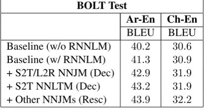
Results are shown in Table 4. The baseline here uses the same feature set as the strong NIST sys-tem. On Arabic, the total gain is +2.6 BLEU, while on Chinese, the gain is +1.3 BLEU.

BOLT Test

Ar-En Ch-En

BLEU BLEU Baseline (w/o RNNLM) 40.2 30.6 Baseline (w/ RNNLM) 41.3 30.9 + S2T/L2R NNJM (Dec) 42.9 31.9

+ S2T NNLTM (Dec) 43.2 31.9

+ Other NNJMs (Resc) 43.9 32.2 Table 4: Primary results on Arabic-English and Chinese-English BOLT Web Forum. Each row includes the aggregate features from all previous rows.

6.4 Effect ofk-best Rescoring Only

Table 5 shows performance when our S2T/L2R NNJM is used only in 1000-best rescoring, com-pared to decoding. The primary purpose of this is as a comparison to Le et al. (2012), whose model can only be used ink-best rescoring.

BOLT Test

Ar-En

Without With RNNLM RNNLM

BLEU BLEU

Baseline 40.2 41.3

S2T/L2R NNJM (Resc) 41.7 41.6 S2T/L2R NNJM (Dec) 42.8 42.9 Table 5: Comparison of our primary NNJM in de-coding vs. 1000-best rescoring.

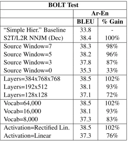
6.5 Effect of Neural Network Configuration

Table 6 shows results using the S2T/L2R NNJM with various configurations. We can see that re-ducing the source window size, layer size, or vo-cab size will all degrade results. Increasing the sizes beyond the default NNJM has almost no ef-fect (102%). Also note that the target-only NNLM (i.e., Source Window=0) only obtains 33% of the improvements of the NNJM.

BOLT Test

Ar-En BLEU % Gain

“Simple Hier.” Baseline 33.8

-S2T/L2R NNJM (Dec) 38.4 100%

Source Window=7 38.3 98%

Source Window=5 38.2 96%

Source Window=3 37.8 87%

Source Window=0 35.3 33%

Layers=384x768x768 38.5 102%

Layers=192x512 38.1 93%

Layers=128x128 37.1 72%

Vocab=64,000 38.5 102%

Vocab=16,000 38.1 93%

Vocab=8,000 37.3 83%

Activation=Rectified Lin. 38.5 102%

Activation=Linear 37.3 76%

Table 6: Results with different neural net-work architectures. The “default” NNJM in the second row uses these parameters: SW=11, L=192x512x512, V=32,000, A=tanh. All mod-els use a 3-word target history (i.e., 4-gram LM). “Layers” refers to the size of the word embedding followed by the hidden layers. “Vocab” refers to the size of the input and output vocabularies. “% Gain” is the BLEU gain over the baseline relative to the default NNJM.

6.6 Effect of Speedups

All previous results use a self-normalized neural network with two hidden layers. In Table 7, we compare this to using a standard network (with two hidden layers), as well as a pre-computed neu-ral network.13 _{The “Simple Hierarchical”}

base-line is used here because it more closely approx-imates a real-time MT engine. For the sake of speed, these experiments only use the S2T/L2R NNJM+S2T NNLTM.

13_{The difference in score for self-normalized vs.}

pre-computed isentirelydue to two vs. one hidden layers.

Each result from Table 7 corresponds to a row in Table 2 of Section 2.4. We can see that go-ing from the standard model to the pre-computed model only reduces the BLEU improvement from +6.4 to +6.1, while increasing the NNJM lookup speed by a factor of 10,000x.

BOLT Test

Ar-En BLEU Gain

“Simple Hier.” Baseline 33.8

-Standard NNJM 40.2 +6.4

Self-Norm NNJM 40.1 +6.3

Pre-Computed NNJM 39.9 +6.1

Table 7: Results for the standard NNs vs. self-normalized NNs vs. pre-computed NNs.

In Table 2 we showed that the cost of unique lookups for the pre-computed NNJM is only

∼0.001 seconds per source word. This does not include the cost of n-gram creation or cached lookups, which amount to ∼0.03 seconds per source word in our current implementation.14

However, then-grams created for the NNJM can be shared with the Kneser-Ney LM, which reduces the cost of that feature. Thus, the total cost in-crease of using the NNJM+NNLTM features in decoding is only∼0.01 seconds per source word.

In future work we will provide more detailed analysis regarding the usability of the NNJM in a low-latency, high-throughput MT engine.

7 Related Work

Although there has been a substantial amount of past work in lexicalized joint models (Marino et al., 2006; Crego and Yvon, 2010), nearly all of these papers have used older statistical techniques such as Kneser-Ney or Maximum Entropy. How-ever, not only are these techniques intractable to train with high-order context vectors, they also lack the neural network’s ability to semantically generalize (Mikolov et al., 2013) and learn non-linear relationships.

A number of recent papers have proposed meth-ods for creating neural network translation/joint models, but nearly all of these works have ob-tained much smaller BLEU improvements than ours. For each related paper, we will briefly

con-14_{In our decoder, roughly 95% of NNJMn-gram lookups}

trast their methodology with our own and summa-rize their BLEU improvements using scores taken directly from the cited paper.

Auli et al. (2013) use afixed continuous-space source representation, obtained from LDA (Blei et al., 2003) or a source-only NNLM. Also, their model is recurrent, so it cannot be used in decod-ing. They obtain +0.2 BLEU improvement on top of a target-only NNLM (25.6 vs. 25.8).

Schwenk (2012) predicts an entire target phrase at a time, rather than a word at a time. He obtains +0.3 BLEU improvement (24.8 vs. 25.1).

Zou et al. (2013) estimate context-free bilingual lexical similarity scores, rather than using a large context. They obtain an +0.5 BLEU improvement on Chinese-English (30.0 vs. 30.5).

Kalchbrenner and Blunsom (2013) implement a convolutional recurrent NNJM. They score a 1000-best list using only their model and are able to achieve the same BLEU as using all 12 standard MT features (21.8 vs 21.7). However, additive re-sults are not presented.

The most similar work that we know of is Le et al. (2012). Le’s basic procedure is to re-order the source to match the linear order of the target, and then segment the hypothesis into minimal bilin-gual phrase pairs. Then, he predicts each target word given the previous bilingual phrases. How-ever, Le’s formulation could only be used in k -best rescoring, since it requires long-distance re-ordering and a large target context.

Le’s model does obtain an impressive +1.7 BLEU gain on top of a baseline without an NNLM (25.8 vs. 27.5). However, when compared to the strongest baseline which includes an NNLM, Le’s best models (S2T + T2S) only obtain an +0.6 BLEU improvement (26.9 vs. 27.5). This is con-sistent with our rescoring-only result, which indi-cates that k-best rescoring is too shallow to take advantage of the power of a joint model.

Le’s model also uses minimal phrases rather than being purely lexicalized, which has two main downsides: (a) a number of complex, hand-crafted heuristics are required to define phrase boundaries, which may not transfer well to new languages, (b) the effective vocabulary size is much larger, which substantially increases data sparsity issues.

We should note that our best results use six sep-arate models, whereas all previous work only uses one or two models. However, we have demon-strated that we can obtain 50%-80% of the

to-tal improvement with only one model (S2T/L2R NNJM), and 70%-90% with only two models (S2T/L2R NNJM + S2T NNLTM). Thus, the one and two-model conditions still significantly out-perform any past work.

8 Discussion

We have described a novel formulation for a neural network-based machine translation joint model, along with several simple variations of this model. When used as MT decoding features, these models are able to produce a gain of +3.0 BLEU on top of a very strong and feature-rich baseline, as well as a +6.3 BLEU gain on top of a simpler system.

Our model is remarkably simple – it requires no linguistic resources, no feature engineering, and only a handful of hyper-parameters. It also has no reliance on potentially fragile outside algorithms, such as unsupervised word clustering. We con-sider the simplicity to be a major advantage. Not only does this suggest that it will generalize well to new language pairs and domains, but it also sug-gests that it will be straightforward for others to replicate these results.

Overall, we believe that the following factors set us apart from past work and allowed us to obtain such significant improvements:

1. The ability to use the NNJM in decoding rather than rescoring.

2. The use of a large bilingual context vector, which is provided to the neural network in “raw” form, rather than as the output of some other algorithm.

3. The fact that the model is purely lexicalized, which avoids both data sparsity and imple-mentation complexity.

4. The large size of the network architecture. 5. The directional variation models.

References

Michael Auli, Michel Galley, Chris Quirk, and Geof-frey Zweig. 2013. Joint language and translation modeling with recurrent neural networks. In Pro-ceedings of the 2013 Conference on Empirical Meth-ods in Natural Language Processing, pages 1044– 1054, Seattle, Washington, USA, October. Associa-tion for ComputaAssocia-tional Linguistics.

Yoshua Bengio, R´ejean Ducharme, Pascal Vincent, and Christian Jauvin. 2003. A neural probabilistic lan-guage model. Journal of Machine Learning Re-search, 3:1137–1155.

David M. Blei, Andrew Y. Ng, and Michael I. Jordan. 2003. Latent dirichlet allocation. J. Mach. Learn. Res., 3:993–1022, March.

David Chiang, Kevin Knight, and Wei Wang. 2009. 11,001 new features for statistical machine transla-tion. InHLT-NAACL, pages 218–226.

David Chiang. 2007. Hierarchical phrase-based trans-lation. Computational Linguistics, 33(2):201–228.

Josep Maria Crego and Franc¸ois Yvon. 2010. Factored bilingualn-gram language models for statistical ma-chine translation. Machine Translation, 24(2):159– 175.

Jacob Devlin and Spyros Matsoukas. 2012. Trait-based hypothesis selection for machine translation. InProceedings of the 2012 Conference of the North American Chapter of the Association for Computa-tional Linguistics: Human Language Technologies, NAACL HLT ’12, pages 528–532, Stroudsburg, PA, USA. Association for Computational Linguistics.

Jacob Devlin. 2009. Lexical features for statistical machine translation. Master’s thesis, University of Maryland.

Nizar Habash, Ryan Roth, Owen Rambow, Ramy Es-kander, and Nadi Tomeh. 2013. Morphological analysis and disambiguation for dialectal arabic. In

HLT-NAACL, pages 426–432.

Zhongqiang Huang, Jacob Devlin, and Rabih Zbib. 2013. Factored soft source syntactic constraints for hierarchical machine translation. InEMNLP, pages 556–566.

Nal Kalchbrenner and Phil Blunsom. 2013. Recurrent continuous translation models.

Reinhard Kneser and Hermann Ney. 1995. Im-proved backing-off for m-gram language modeling. InAcoustics, Speech, and Signal Processing, 1995. ICASSP-95., 1995 International Conference on, vol-ume 1, pages 181–184. IEEE.

Hai-Son Le, Alexandre Allauzen, and Franc¸ois Yvon. 2012. Continuous space translation models with

neural networks. In Proceedings of the 2012 Con-ference of the North American Chapter of the Asso-ciation for Computational Linguistics: Human Lan-guage Technologies, NAACL HLT ’12, pages 39– 48, Stroudsburg, PA, USA. Association for Compu-tational Linguistics.

Yann LeCun, L´eon Bottou, Genevieve B Orr, and Klaus-Robert M¨uller. 1998. Efficient backprop. In

Neural networks: Tricks of the trade, pages 9–50. Springer.

Jos´e B Marino, Rafael E Banchs, Josep M Crego, Adri`a De Gispert, Patrik Lambert, Jos´e AR Fonollosa, and Marta R Costa-Juss`a. 2006. N-gram-based machine translation. Computational Linguistics, 32(4):527– 549.

Tomas Mikolov, Martin Karafi´at, Lukas Burget, Jan Cernock´y, and Sanjeev Khudanpur. 2010. Recur-rent neural network based language model. In IN-TERSPEECH, pages 1045–1048.

Tomas Mikolov, Wen tau Yih, and Geoffrey Zweig. 2013. Linguistic regularities in continuous space word representations. InHLT-NAACL, pages 746– 751.

Franz Josef Och and Hermann Ney. 2003. A sys-tematic comparison of various statistical alignment models. Computational Linguistics, 29(1):19–51. Razvan Pascanu, Tomas Mikolov, and Yoshua Bengio.

2012. On the difficulty of training recurrent neural networks. arXiv preprint arXiv:1211.5063.

Jason Riesa, Ann Irvine, and Daniel Marcu. 2011. Feature-rich language-independent syntax-based alignment for statistical machine translation. In

Proceedings of the Conference on Empirical Meth-ods in Natural Language Processing, EMNLP ’11, pages 497–507, Stroudsburg, PA, USA. Association for Computational Linguistics.

Ronald Rosenfeld. 1996. A maximum entropy ap-proach to adaptive statistical language modeling.

Computer, Speech and Language, 10:187–228.

Antti Rosti, Bing Zhang, Spyros Matsoukas, and Rich Schwartz. 2010. BBN system descrip-tion for WMT10 system combinadescrip-tion task. In

WMT/MetricsMATR, pages 321–326.

Holger Schwenk. 2010. Continuous-space language models for statistical machine translation. Prague Bull. Math. Linguistics, 93:137–146.

Holger Schwenk. 2012. Continuous space translation models for phrase-based statistical machine transla-tion. InCOLING (Posters), pages 1071–1080. Libin Shen, Jinxi Xu, and Ralph Weischedel. 2010.

Matthew Snover, Bonnie Dorr, and Richard Schwartz. 2008. Language and translation model adaptation using comparable corpora. In Proceedings of the Conference on Empirical Methods in Natural Lan-guage Processing, EMNLP ’08, pages 857–866, Stroudsburg, PA, USA. Association for Computa-tional Linguistics.

Makoto Tanaka, Yasuhara Toru, Jun-ya Yamamoto, and Mikio Norimatsu. 2013. An efficient language model using double-array structures.

Ashish Vaswani, Yinggong Zhao, Victoria Fossum, and David Chiang. 2013. Decoding with large-scale neural language models improves translation. In Proceedings of the 2013 Conference on Em-pirical Methods in Natural Language Processing, pages 1387–1392, Seattle, Washington, USA, Oc-tober. Association for Computational Linguistics. Will Y Zou, Richard Socher, Daniel Cer, and