Nonparametric Dynamic Conditional Beta

Munich Personal RePEc Archive

Nonparametric Dynamic Conditional

Beta

Maheu, John M and Shamsi, Azam

McMaster University, McMaster University

16 September 2016

Online at

https://mpra.ub.uni-muenchen.de/77424/

Nonparametric Dynamic Conditional Beta

∗

John M. Maheu

Azam Shamsi

February 2017

Abstract

This paper derives a dynamic conditional beta representation using a Bayesian semiparametric multivariate GARCH model. The conditional joint distribution of excess stock returns and market excess returns are modeled as a countably infinite mixture of normals. This allows for deviations from the elliptic family of distribu-tions. Empirically we find the time-varying beta of a stock nonlinearly depends on the contemporaneous value of excess market returns. In highly volatile markets, beta is almost constant, while in stable markets, the beta coefficient can depend asymmetrically on the market excess return.

Key words: Dirichlet Process Mixture; GARCH; Beta.

∗_{Maheu thanks the SSHRC of Canada for financial support. We are grateful for comments from Ron}

Balvers, Martin Burda and Jia Liu. We thank participants of the CFE 2015 conference, Melbourne Bayesian Econometric Workshop 2015 and the Doctoral Workshop in Applied Econometrics, University of Toronto 2016 for helpful comments.

†_{DeGroote School of Business, McMaster University, Hamilton, ON, Canada. E-mail address:}

[email protected].

‡_{DeGroote School of Business, McMaster University, Hamilton, ON, Canada. E-mail address:}

1

Introduction

This paper shows how to nonparametrically estimates the dynamic conditional beta of a stock using a Bayesian semiparametric multivariate GARCH model. This extends Engle’s (2016) parametric version of dynamic conditional beta to the case of an unknown general continuous distribution. In this setting the whole distribution can affect the compensation for risk.

Researchers have long studied the beta coefficient of a stock which represents the nondiversifiable risk arising from exposure to market movements. Traditional approaches estimate the beta coefficient by regressing excess stock returns on the excess market return as in the one-factor Capital Asset Pricing Model (CAPM, Sharpe (1964) and Lintner (1965)), or exploiting more empirically supported asset pricing models, such as Fama-French three-factor model, which incorporate additional explanatory variables (Fama & French (1993)). Our multivariate model nests both cases, but allows for time variation in the conditional second moments. There is a large literature based on multivariate GARCH (MGARCH) models that link a time varying beta to the conditional second moments. Some examples include Bollerslev et al. (1988),Giannopoulos (1995), McCurdy & Morgan (1992) and Choudhry (2002).

Recently Engle (2016) proposes a multivariate normal GARCH model from which the conditional distribution defines the dynamic beta coefficient. This directly links time-varying second moments to the time-time-varying beta in a consistent fashion. The parametric pricing relationship holds more generally for the elliptic family of distributions. This is an attractive approach but may be limiting if the parametric distributional assumptions are not valid.

A key insight of our approach is that if the joint distribution of excess stock returns and market returns are correctly specified then it follows that their contemporaneous pricing relationship is completely determined by the associated conditional distribution. Therefore, we semiparametrically model the conditional distribution as a countably in-finite mixture of multivariate normals. Each normal component in the mixture has a conditional covariance directed by a MGARCH process. Our model nests the Gaussian and Student-t distribution as special cases but importantly allows for deviations from the elliptic family of distributions. This includes asymmetric distributions which the el-liptic family omit being only symmetric. The mixing is over both the mean vector and covariance matrix.

We follow Jensen and Maheu (2013) to implement a Bayesian semi-parametric MGARCH model and extend it to allow for asymmetric shocks in volatility. The data strongly support the semiparametric MGARCH specification over Gaussian and Student-t distributional alternatives.

In this framework, the conditional distribution of stock returns given the market excess return (and possibly other factors) can be represented as an infinite mixture with weights written as functions of the value of the market excess return. Consequently, the beta coefficient of a security at each time will depend nonparametrically on the contemporaneous value of market return, as opposed to the beta derived from existing models which is insensitive to the contemporaneous value of the market return.

the individual stock return derived from models with different dimensions and is directly comparable across specifications. Empirically, the one factor model is strongly supported for all stocks compared to specifications with Fama-French factors and momentum.

Although the time series of the realized conditional betas from the semiparametric model are similar to the benchmark model, we find significant nonlinear dependence in beta as a function of the contemporaneous value of the market excess return. In the parametric models, beta is constant as a function of the market excess return.

When the market is highly volatile, beta is not affected by unexpected shocks in the market return. While in a calm market, beta can change dramatically from unexpected shocks. For stocks which are highly correlated with the market, an unexpected shock during calm periods increases the beta coefficient. The effect is the reverse for the stocks with low correlation with the market. In other words, when an asset is highly correlated with the market, large moves in a stable market increase the conditional covariance between the market and the asset more than they increase the conditional variance of the market, resulting in a significant increase in the beta coefficient. When an asset has low conditional correlation with the market, large moves in a stable market increase the conditional variance of the market more than they increase the conditional covariance between the market and the asset, leading to a drop in conditional beta. These are important contemporaneous nonlinear dynamics that are absent in other models.

The remainder of the paper is structured as follows. We begin by reviewing the benchmark model which is an MGARCH model with Student-t innovations. Section 3 provides a general theoretical setting of the multivariate model used in this study, key fea-tures of the semiparametric MGARCH model, and the use of the Dirichlet process prior. Posterior sampling is detailed in Section 4. The derivation of the nonparametric dynamic conditional beta is presented in Section 5. Data is introduced in Section 6, and Section 7 assesses models with different number of factors and compares the performance of the proposed model to the benchmark model. Applications of the semiparametric model are found in Section 8, and Section 9 provides some implications of the semiparametric model in finance. Section 10 concludes and an Appendix defines distributions and collects the detailed derivations.

2

Benchmark Model

Our benchmark model is a straightforward extension of Engle (2016). Engle (2016) defines dynamic conditional beta using a multivariate GARCH (MGARCH) model assuming a multivariate normal distribution as the joint density of stock returns and factors. We replace the normal distribution with a Student-t to accommodate the fat-tails in the data. Let the excess stock return on asset iberi,t and a vector of regressors (factors) including the excess market return be rf,t = (rf1,t, rf2,t, ..., rfq,t)

′

. rt = (ri,t, r′_f,t)′ _{is assumed to}

follow the MGARCH-t

rt|r1:t−1 ∼t(µ, Ht, ν), (2.1)

Ht= Γ0+ Γ1⊙(rt−1 −η)(rt−1−η)′+ Γ2⊙Ht−1, (2.2)

wheret(µ,Σ, ν) denotes a t-distribution (see appendix) with mean vectorµ, scale matrix Σ and degree of freedom ν and r1:t−1 = {r1, . . . , rt−1} is the information set available at

time t−1. The scale matrix, Ht, is based on the vector-diagonal multivariate GARCH

symbol ⊙ denotes the Hadamard product. The parameter is Γ = {Γ0,Γ1,Γ2, η}, with

the symmetric positive definite matrices parameterized as Γ0 = Γ1/20 (Γ 1/2

0 )′, Γ1 =γ1(γ1)′,

and Γ2 = γ2(γ2)′ where Γ0 is a lower triangular (q+ 1)×(q+ 1) matrix and γ1, γ2 and η are (q+ 1)-vectors. η permits a nonlinear asymmetric response to shocks and can be considered a multivariate version of the asymmetric GARCH model (Engle & Ng 1993).

Partition rt = (r′ 1,t, r

′ 2,t)

′

into a k1 and k2 (k1 +k2 = q+ 1) vector and similarly

µ= (µ′ 1, µ

′ 2)

′

and

Ht=hH11,tH12,t H12,tH22,t i

.

Applying the properties of the Student-t distribution (Roth 2013) the conditional distri-bution of r1,t givenr2,t is

r1,t|r2,t ∼ t(µ1|2, Ht,1|2, ν1|2), (2.3)

µ1|2 = µ1+H12,tH22,t−1(r2,t−µ2), (2.4)

Ht,1|2 = ν+ (r2,t−µ2)

′

H_22,t−1(r2,t−µ2)

ν+k2 (H11,t−H12,tH

−1 22,tH

′

12,t), (2.5)

ν1|2 = ν+k2, (2.6)

where the conditional mean is µ1|2, the conditional scale matrix is Ht,1|2 and the degree of freedom ν1|2.

This is a useful result in that it tells us how the conditional distribution ofr1,t reacts to any value of r2,t. For instance, if r1,t ≡ri,t and conditioning on one factor, the excess market return, r2,t ≡rm,t, substituting into (2.4) directly gives a dynamic risk premium

for asset i as

E[ri,t|rm,t, Ht] =µi +H12,tH_22,t−1(rm,t−µm). (2.7)

This tells how the expected excess return of asset i reacts to any value of the market. If the market shock is zero (rm,t = µm) then the expected value is µi but for all other realizations the market shock impacts the expected return of the asset. Engle identifies the dynamic conditional beta that arises from the joint relationship as

βt =H12,tH_22,t−1. (2.8)

This is the derivative of (2.7) with respect to rm,t. A conditional pricing relationship is

obtained by setting r2,t ≡E[rm,t|r1:t−1] and substituting into (2.7).

There are several advantages to modeling excess returns in this way. First, it confronts the simultaneous nature of the asset return and the factors that price the risk premium. Rather than specifying a single equation partial equilibrium relationship the model begins with the full joint dynamics. Second, the joint distribution of the asset and the factors directly pins down the conditional distribution and the implications for the risk premium. The dynamic beta is a function of the conditional covariance matrix. This is a general result that holds for the elliptic family of distributions.

We estimate the model from a Bayesian perspective. The posterior density has the non-standard form

p(µ,Γ, ν|r1:T)∝p(ν)p(µ)p(Γ)×

T Y

t=1

where t(rt|µ, Ht, ν) is the density of the Student-t distribution, and p(ν)p(µ)p(Γ) is the

prior density for µ,Γ, ν. Posterior draws of the parameters vector are simulated with a Metropolis-Hastings sampler.

Although attractive, the conditional distribution in (2.3) has some drawbacks. The conditional beta derived from MGARCH-t model, at each time, is constant with respect to the contemporaneous value of market return (Equation 2.8), and consequently, the conditional expected return of the stock is a linear function of the factor returns. This pricing relationship will not hold for more general distributions not belonging to the elliptic family. The elliptic family of distributions are symmetric about their mean and do not account for asymmetry observed in financial returns.

This model imposes a strong assumption on the functional form of the joint distri-bution of the data. In this paper, we remove this restrictive assumption by employing a Dirichlet process mixture (DPM) to model the unknown joint distribution of returns. This results in a potentially non-constant conditional beta and a nonlinear conditional expected return of the stock as a function of the contemporaneous value of the market return.

3

A Bayesian Semiparametric Model

Unlike the benchmark model that assumes a specific parametric joint distribution for the individual asset returns and the factors, we model this joint distribution nonparametri-cally by an infinite mixture of normal distributions which can approximate any continuous multivariate distribution. Recall thatrt= (ri,t, rf1,t, ..., rfq,t)

′ _{represents the excess return}

vector of an individual stock and q factors at time t. The infinite mixture representation can be written as

rt|Ht, µ, B, W ∼ ∞ X

j=1

ωjN(µj,(H_t1/2)Bj(H_t1/2)′). (3.1)

whereHt1/2 is the Cholesky decomposition ofHt,µ={µ1, µ2, . . .},B ={B1, B2, . . .}and W ={ω1, ω2, . . .}is the vector of the weights, such thatωj ≥0 for allj andP∞_j=1ωj = 1.

The mixing is over the mean vector and the componentBj of the covariance matrix. The

second component, Ht of the covariance matrix captures volatility clustering through

time but is not a function of j. Bj is a symmetric positive definite matrix which scales

Ht to yield a better estimate of the joint density of data. Given Ht, in general any

positive definite matrix Ht1/2Bj(H 1/2

t )′ can be represented with the appropriate choice of Bj making this a very flexible structure.

The conditional mean can be derived in exactly the same way as in the benchmark model except it will follow an infinite mixture of conditional normal distributions. If

rf t = (rf1,t, ..., rfq,t) ′

then the conditional density ofri,t givenrf,t is a mixture distribution as well and the conditional expectation can be written as the following weighted mixture

E(ri,t|rf,t, Ht) =

∞ X

j=1

qj(rf,t)E(ri,t|rf,t, µj, Bj, Ht). (3.2)

model the conditional expectation is not a linear function of the factors. To obtain the nonparametric conditional beta, we take the derivative of (3.2) with respect to the desired factor. The conditional beta is not constant in general but it changes as the con-temporaneous value of the corresponding factor changes. The next section introduces the Dirichlet process prior to estimate this model. In Section 5 we derive the nonparametric conditional beta.

In Bayesian inference the Dirichlet process (DP) prior (Ferguson 1973) is a stan-dard prior used for infinite dimensional objects such as (3.1). A draw from a DP,

G ∼ DP(α, G0), is almost surely a discrete distribution and is governed by two pa-rameters. The concentration parameter α, a positive scalar and a base distribution G0. The nonparametric distribution Gis centered on the base distribution G0, which can be considered as the prior guess; E(G) = G0. The concentration parameter measures the strength of belief in G0. The larger α, the stronger belief in G0 and the more distinct elements we have with non-negligible mass. Lo (1984) introduces Dirichlet process

mix-ture (DPM) model in which G is the mixing measure over a continuous kernel. This

has become a standard Bayesian approach to nonparametric estimation of an unknown continuous distribution. In this paper, G is the unknown distribution that governs the mixing over the mean vector and covariance matrix of the normal kernel in our mixture model.

The model (MGARCH-DPM) is an extension of Jensen & Maheu (2013) and allows for asymmetry in the MGARCH process from shocks to volatility and fat tails without making any restrictive assumption. The hierarchical form of the model is,

rt|φt, Ht ∼ N(ξt, H_t1/2Λt(Ht1/2)′), t= 1, ..., T (3.3)

φt ≡ {ξt,Λt}|G∼G, (3.4)

G|α, G0 ∼ DP(α, G0), (3.5)

G0 ≡ N(µ0, D)× W−1(B0, ν0), (3.6)

Ht = Γ0+ Γ1⊙(rt−1−η)(rt−1−η)′+ Γ2⊙Ht−1. (3.7)

In this modelξtis a (q+1)-vector and Λtis a symmetric positive definite matrix andHt

fol-lows the same MGARCH specification as the benchmark parametric model. W−1_{(B0, ν0)}

represents an inverse Wishart distribution (see appendix) with scale matrixB0 and degree of freedom ν0.

Sethuraman (1994) characterizes a stick-breaking representation of the DP. Com-bining this with the normal kernel gives the associated stick breaking representation of the MGARCH-DPM density as

p(rt|µ, B, W, Ht) =

∞ X

j=1

ωjN(rt|µj, Ht1/2Bj(H 1/2

t )′), (3.8)

ω1 = v1, ωj =vj j−1 Y

l=1

(1−vl), j >1, (3.9)

vj iid∼ Beta(1, α), (3.10)

µj iid∼ N(µ0, D), Bj iid∼ W−1(B0, ν0), (3.11)

whereN(rt|µj, Ht1/2Bj(H 1/2

t )′) denotes the multivariate normal density with meanµj and

of support in the discrete distribution G while ξt and Λt denote draws from G in (3.4),

with the possibility of repeated draws of µj and Bj.

The model nests several special cases. First, the Gaussian model is obtained when

α→0 as ω1 = 1, ωj = 0,∀j >1 andB1 =I. The Student-t model results from µj being

constant for all j and α → ∞, since G→G0, the inverse Wishart distribution.

4

Posterior Sampling

To estimate the unknown parameters in (3.3)-(3.7), we apply an MCMC sampler along with the slice sampler of Walker (2007) and Kalli et al. (2011). Slice sampling introduces a latent variable, ut ∈ (0,1), to elegantly convert an infinite sum to a finite mixture

model which makes the sampling feasible. Estimating the joint posterior density of ut

and other model parameters and then integrating out the slice variable ut recovers the desired posterior density. In practice, this means jointly sampling all parameters including the slice variable but then discarding ut. Define ut such that the joint density of (rt, ut) given (W,Θ≡(µ, B)) is given by

f(rt, ut|W,Θ) = ∞ X

j=1

1(ut< ωj)N(rt|µj,(Ht1/2)′BjHt1/2). (4.1)

Let s1:T = {s1, ..., sT} be the configuration set that partitions the data r1:T into

c distinct clusters such that observation rt is assigned parameter θst = (µst, Bst). Let nj ={#t|st =j} be the number of observations allocated to state j. The full likelihood is

p(r1:T, u1:T, s1:T|W,Θ) = ΠTt=11(ut< ωst)N(rt|µst,(H 1/2

t )Bst(H 1/2

t )′), (4.2)

and the joint posterior is proportional to

p(W1:K)ΠK_j=1p(µj, Bj)ΠT_t=11(ut < ωst)N(rt|µst,(H 1/2

t )Bst(H 1/2

t )′) (4.3)

where K is the smallest natural number that satisfies the condition PK_j=1ωj > 1 −

min{ut}T

t=1 andW1:K denotes the finite set ofW and similarly for other parameters µ1:K

and B1:K. Having defined the notation, the steps of the MCMC algorithm are discussed

next.

Steps of MCMC algorithm for MGARCH-DPM

1. The posterior distribution of θj = (µj, Bj), j = 1, ..., K: Using the transformation

zt=Ht−1/2rt, and applying the results of conditionally conjugate priors for the linear

regression model we have

Bj|r1:T, s1:T, µj,Γ ∼ W−1 nj+ν0, B0+X

st=j

(zt−Ht−1/2µj)(zt−H −1/2 t µj)′

!

(4.4)

µj|r1:T, s1:T, Bj,Γ ∼ N(¯µ,D¯) (4.5)

in which

¯

D−1 =D−1+ X

t|st=j

Ht−1/2′Bj−1H −1/2

t , µ¯= ¯D 

X

t|st=j

Ht−1/2′Bj−1zt+D−1µ0 

2. Updatingvj, j = 1, ..., K.

vj|S∼Beta 1 +

T X

t=1

1(st=j), α+

T X

t=1

1(st> j)

!

. (4.7)

Then we update W1:K based on (3.9).

3. Updating ut, t = 1, ..., T. ut|s1:T ∼ U(0, ωst). Then update K such that PK

j=1ωj >

1−min{ut}T

t=1. Additional ωj and θj will need to be generated from the priors if K

is incremented.

4. Updatings1:T. For eacht= 1, ..., T,

p(st=j|r1:T)∝1(ωj > ut)N(rt|µj, H_t1/2Bj(H_t1/2)′), j = 1, ..., K. (4.8)

5. Updatingα: Assuming a gamma priorα∼ G(a0, b0) (see appendix)αcan be sampled following the two steps below (Escobar & West 1995). Recall that c is the number of alive clusters defined as the number of clusters in which at least one observation is allocated. Note that c≤K. Then the sampling steps are as follows.

(a) (τ|α, c)∼Beta(α+ 1, T).

(b) Sample α from

α|τ ∼πτG(a0+c, b0−log(τ)) + (1−πτ)G(a0+c−1, b0−log(τ)),

where πτ is defined by πτ 1−πτ =

a0+c−1

T(b0−log(τ)).

6. Updating GARCH parameters Γ = (Γ1/2₀ , γ1, γ2, η). The conditional posterior is

p(Γ|µ, B, S, r1:T, H1:T)∝p(Γ)×

T Y

t=1

N(rt|µst, H 1/2 t Bst(H

1/2

t )′) (4.9)

which is not of standard form, and we apply a Metropolis-Hastings sampler. Given the current value Γ of the chain, the proposal Γ′ _{is sampled Γ}′ _{∼N(Γ,Vb). The draw}

is accepted with probability

min{p(Γ′|µ, B, S, r1:T, H1:T)/p(Γ|µ, B, S, r1:T, H1:T),1},

and otherwise rejected. Vb is proportional to the inverse Hessian matrix of ℓ =

log[p(Γ|µ, B, S, r1:T, H1:T)] evaluated at its posterior mode,bΓ, which is computed once

at the start of estimation. Vb is scaled to achieve an acceptance rate between 0.2

and 0.5. In this paper we apply the numerical optimization of the

Broyden-Fletcher-Goldfarb-Shanno (BFGS) algorithm to approximate the posterior mode of ℓ.

5

Nonparametric Dynamic Conditional Beta

sampling algorithm, we sample model parameters for many iterations and after dropping a set of burn-in draws we have the following set of sampled parameters:

{(µ(g)_j , B_j(g)), v_j(g), j = 1, ..., K(g)},{s(g)t , u (g)

t , t= 1, ..., T}, H (g) 1:T ={H

(g) 1 , ..., H

(g)

T }, (5.1)

for g = 1, ..., M where M is the number of MCMC iterations. At each iteration g = 1, ..., M of the algorithm, a draw of G|r1:T, can be written as

G(g)=

K(g)

X

j=1

ω(g)_j δ_θ(g)

j +

 1−

K(g)

X

j=1 ω_j(g)



G0(θ), (5.2)

where θ(g)_j = (µ(g)_j , B_j(g)) and δ_θ(g)

j is a mass point at θ (g) j .

Combining this with the normal kernel gives the predictive density for the generic return (ri,t,rm,t) conditional on G(g) as

p(r_i,t,r_m,t|r1:T, G(g)) = K(g)

X

j=1

ω_j(g)f(r_i,t,r_m,t|θ_j(g)) +

 1−

K(g)

X

j=1 ω_j(g)



Z f(r_i,t,r_m,t|θ)G0(θ)dθ,

(5.3) where f(ri,t,rm,t|θ) is the multivariate normal density.

To assess the nonlinear regression function E(ri,t|rm,t, r1:T), or the conditional beta of the individual stock i, we require the conditional density derived from this predictive (joint) density of (ri,t,rm,t). Therefore,

p(ri,t|rm,t, r1:T, G(g)) = p(ri,t,rm,t|r1:T, G

(g)₎

p(rm,t|r1:T, G(g)₎ (5.4)

= p(ri,t,rm,t|r1:T, G

(g)₎ PK(g)

j=1 ω (g)

j f2(rm,t|θ (g) j ) +

1−PK_j=1(g)ω(g)_j R f2(rm,t|θ)G0(θ)dθ

=

K(g)

X

j=1

q(g)_j (rm,t)f(ri,t|rm,t, θj(g)) +  1−

K(g)

X

j=1

q_j(g)(rm,t) 

f(ri,t|rm,t, G0), (5.5)

where

q_j(g)(rm,t) =

ω_j(g)f2(rm,t|θ_j(g))

PK(g)

j=1 ω (g)

j f2(rm,t|θ(g)j ) +

1−PK_j=1(g)ω_j(g) R f2(rm,t|θ)G0(θ)dθ

(5.6)

and f2(rm,t|θ_j(g)) is the marginal (normal) density of rm,t and f(ri,t|rm,t, G0) is the

con-ditional distribution using the base measure. The terms q_j(g)(r_m,t) determine which components in the mixture receive more weight. Clusters that have a marginal den-sity f2(rm,t|θ_j(g)) that has a higher likelihood value for rm,t will receive larger weights.

The marginal density, and hence relative weight of clusters, will change with r_m,t as well

as over time through the MGARCH component, Ht. These features will determine the

Our focus is on the conditional mean of r_i,t given r_m,t. Using the properties of the normal distribution the conditional mean directly comes from (5.5) and is

E(ri,t|rm,t, r1:T, G(g)) =

K(g)

X

j=1

q_j(g)(rm,t)[µ(g)j,1 +β (g)

jt (rm,t−µ(g)j,2)]+ (5.7)

 1−

K(g)

X

j=1

q_j(g)(rm,t)   R

[µ1+βt(rm,t−µ2)]N(rm,t|µ2,(H(g)

1/2

t BH

(g)1/2′

t )22)p(µ, B)dµdB R

N(rm,t|µ2,(H_t(g)1/2BH_t(g)1/2′)22)p(µ, B)dµdB

.

The cluster specific beta is defined as

β_jt(g) = (H

(g)1/2

t BjH(g)

1/2′ t )12

(Ht(g)1/2BjH (g)1/2′ t )22

(5.8)

where the subscript (i, j) on ()ij denotes element (i, j) of the matrix and βt in the

sec-ond line of (5.7) is defined as β_jt(g) except Bj is replaced with B. The numerator and

denominator in the last term of (5.7) can be approximated by simulation.

Integrating all parameter and distributional uncertainty results in an estimate of the predictive conditional mean as

E(ri,t|rm,t, r1:T)≈ 1 M

M X

g=1

E(ri,t|rm,t, r1:T, G(g)). (5.9)

The predictive mean of the conditional beta is the derivative of this conditional expecta-tion of ri,t given rm,t, (5.9) with respect to rm,t. This is,

bm,t(rm,t) =

∂E(ri,t|rm,t, r1:T)

∂rm,t

rm,t=rm,t

. (5.10)

Full details on this derivative and estimate are provided in the appendix.

In the case that we have more than one factor, we follow the same process. We first estimate the joint model and back out the conditional distribution of the stock returnri,t

given all factors. The nonparametric conditional beta in this case is a vector. It is defined analogously to (5.10) as the partial derivative with respect to the factor. For instance in the case of the Fama-French 3-factor model (Fama & French 1993), beta for size factor is defined as

bSM B,t = ∂E(ri,t|rm,t, rSM B,t, rt,HM L, r1:T)

∂rSM B,t

rm,t=rm,t rSM B,t=rSM B,t rHM L,t=rHM L,t

(5.11)

with a similar expression for the other factor coefficients bm,t and bHM L,t.

6

Data

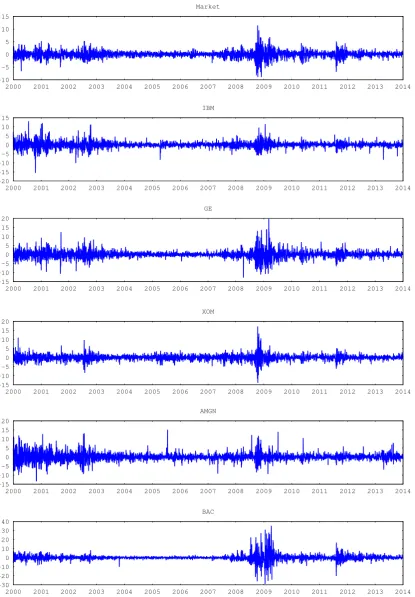
(3521 daily observations). Excess returns are derived after subtracting the risk-free re-turn approximated by the three-month Treasury bill rate. All rere-turns are scaled by 100. Figure 1 displays the data and Table 1 reports summary statistics. All individual stocks display skewness and excess kurtosis. Figure 1 shows that returns with absolute large (small) value tend to be followed by other large (small) absolute returns reflecting volatil-ity clustering. Daily data for the size factor,rSM B,t, value factor,rHM L,t, and momentum factor, rM OM,t, are obtained from Kenneth French’s website.

7

Model Performance

The criteria that we use to compare different models is the value of the log-predictive

likelihood. For each particular model M (i.e., MGARCH-t or MGARCH-DPM), the

predictive likelihood forrL:T,L < T is expressed in terms of the one-step-ahead predictive likelihoods,

m(rL:T|r1:L−1,M) = ΠT_t=Lp(rt|r1:t−1,M) (7.1)

where L >1 is chosen to eliminate the influence of the priors on model comparison. We can approximate the one-step-ahead predictive likelihoods, p(rt|r1:t−1,M), by averaging the data density over draws of the unknown parameters conditional on the data history

r1:t−1. This integrates out parameter and distributional uncertainty as

p(rt|r1:t−1,M) =

Z

p(rt|θ, r1:t−1,M)p(θ|r1:t−1,M)dθ (7.2)

≈ 1

M M X

g=1

p(rt|θ(g), r1:t−1,M)

where θ(g) _{is a posterior draw from p(θ|r1:t−1,M) and p(rt|θ}(g)_{, r1:t−1,M) is the data}

density givenθ(g) _{and r1:t−1 for model M.}

The following priors are used in estimation. In the MGARCH-t model, ν ∼

U(2,100), and µ ∼ N(0,0.1I) for both models. For each of GARCH parameters in both models, we set Γ1/2_0,ij ∼ N(0,100)1S, γ1,i ∼ N(0,100)1S and γ1,i ∼ N(0,100)1S, i = 1, . . . , q + 1, j ≤ i as prior distribution where S denotes the following restriction: diag(Γ1/20 )>0, γ11>0, γ22>0 to impose identification. For the concentration parameter α ∼ G(0.1,0.3) with a mean of 1/3. The prior on α controls the number of the distinct components in the mixture model, although with a large number of observations the ef-fect of the prior is diminished. For the hyper-parameters of the base measure G0, we set

B0 = (ν0−q−1)I which makes E(B) = I and centers the conditional covariance of rt

atHt. ν0 = 8, but other values for ν0 do not change our conclusions.

Based on (7.2), the predictive likelihoods for the two models are estimated as

p(rt|r1:t−1,MGARCH-t) ≈ 1 M

M X

g=1

t(rt|µ(g), Ht(g), ν(g)), (7.3)

p(rt|r1:t−1,MGARCH-DPM) ≈ 1 M

M X

g=1

N(rt|µ(g) s(_tg), H

(g)1/2

t B

(g) s(_tg)H

(g)1/2′

t ). (7.4)

Note that we are able to computeHt(g)at each iteration of the MCMC since we have H_t−1(g) and GARCH parameters: H_t(g)= Γ(g)₀ + Γ(g)₁ ⊙(rt−1−η(g))(r−η(g))′t−1+ Γ

(g)

2 ⊙H

In MGARCH-DPM model, at each iteration g, s(g)t is drawn from one of the K(g) + 1

components with weights ω(g)_j j = 1, . . . , K(g) _{and 1−}PK(g) j=1 ω

(g)

j . When s

(g)

t =K(g)+ 1

a new parameter θ∼G0 is drawn.

To determine the factors to be used, we compare the values of the marginal

pre-dictive likelihood of the individual stock return derived from each model, using different factors. The predictive likelihoods discussed above are directly comparable but when com-paring a model with 2 factors versus 3 factors the independent variablertis 2 dimensional and 3 dimensional, respectively. These predictive likelihood values are not comparable. Instead we compare the marginal predictive likelihood for the individual stock return only. This is obtained from each full model after integrating out the factors in each model. For instance, for excess stock return i we compare the one-factor model against the two-factor model withp(ri,t|ri,1:t−1, rf1,1:t−1) andp(ri,t|ri,1:t−1, rf1,1:t−1, rf2,1:t−1). These

marginal predictive likelihoods are derived from the full predictive likelihood. For exam-ple, the first one is obtained from p(ri,t, rf1,t|ri,1:t−1, rf1,1:t−1) by marginalizing out rf1,t.

This can be done directly on the terms (7.3) and (7.4) by selecting the associated uni-variate marginal density from the multiuni-variate Student-t and normal on the right hand side of these equations.

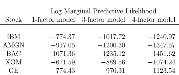
We first compare the performance of the MGARCH-DPM model with different factors. These factors include market excess return, size factor and value factor from the Fama-French 3-factor model, and the momentum factor. The set of factors can be extended to include any factor. Table 2 reports the marginal log-predictive likelihood of IBM, BAC, GE, XOM and AMGN, for the MGARCH-DPM model, for 12/03/2012 to 31/12/2013 (500 observations) when we use different factors. The table shows that, for all stocks under study, the 1-factor model with market excess return as the only factor results in a better marginal predictive likelihood compared to the 3 (market, SMB, HML) and 4-factor models (market, SMB, HML, momentum). The evidence for one factor is very strong. For instance, the log-predictive Bayes factor for the 1 factor IBM model against the 3 factor version is 243.35. Therefore the remainder of the empirical results focus on the the 1-factor model.

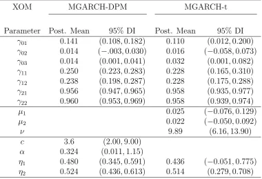
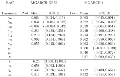
Table 3 reports the log-predictive likelihoods for the 1-factor MGARCH-t and MGARCH-DPM models, and the log-Bayes factor over 12/03/2012 to 31/12/2013. Bi-variate models based on daily excess returns on IBM, GE, XOM, AMGN and BAC each with excess market returns are considered. The results strongly support our semi-parametric model relative to the benchmark model. For instance, log-Bayes factors are all greater than 211. This is very strong evidence of significant deviations from the Student-t MGARCH model.

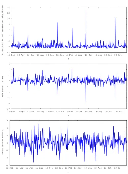
Figure 2 displays the time-series of the market and IBM excess returns as well as the difference in the log-predictive likelihood of the two models using

logp(rt|r1:t−1,MGARCH-DPM)−logp(rt|r1:t−1,MGARCH-t). (7.5)

Positive values favour the MGARCH-DPM specification. This figure shows that the MGARCH-DPM model almost always outperforms MGARCH-t model. There are large differences when the market or IBM returns are extreme.

8

Applications of Semiparametric Conditional Beta

the corresponding counterpart from the parametric MGARCH-t model. Not only does the beta computed in this way change over time, but also the time-varying conditional beta is sensitive to the contemporaneous value of excess market return. This implies that the value of the systematic risk of an asset at each time depends on the level of the market return.

The model is applied to derive a nonparametric conditional beta (calculated in

Section 5) using excess returns on a single stock and on the market return (q = 1).

This results in a conditional expected return of the individual stock comparable to the conditional CAPM model.

The analysis reported here is based on 25000 iterations of the MCMC algorithm. The first 15000 draws were dropped as burn-in and the following 10000 used for inference. The average acceptance rate of GARCH parameters is about 20% and about 30% for parametric and nonparametric models, respectively.

Tables 4-8 report the posterior mean and the 0.95 probability density intervals of the fixed parameters for both models and for different stocks. The estimated MGARCH

parameters from the two models are consistent. The tables report c, the number of

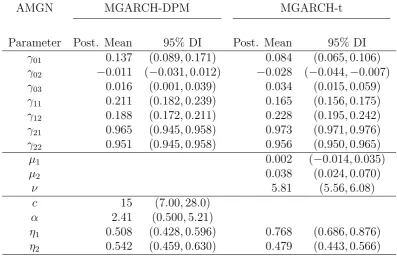
components in the mixture used to estimate the unknown density. On average, the bivariate joint density of IBM, XOM, GE, and BAC with the market is estimated using about 3.6-6.3 components but the density intervals indicate considerable uncertainty. However, for AMGN and the market, about 15 components are used, showing that this joint density is far more complex than the others. These results are compatible with

the small degree of freedom estimated in the benchmark models. Estimates ofη1 and η2

are consistently positive indicating a larger response to the conditional covariance from negative shocks.

Figures 3-7 compare the posterior mean of therealized beta over time derived from both models for each of the stocks. For MGARCH-t model, the posterior mean of (2.8) is reported while for the MGARCH-DPM model the posterior mean of (5.10) is evaluated at the realized excess market return value for timet. As seen in the figures, both models result in very similar time series for the conditional beta.

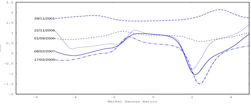
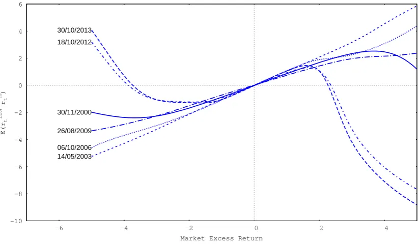
Figures 8-12 illustrate posterior mean of each stock’s conditional beta as a function of the contemporaneous market excess return using (5.10) at several dates. These figures show that beta is changing over time and, more importantly, at each time the value of beta is sensitive to the contemporaneous value of the market excess return. For each stock there are dates that beta is a constant function of the market return which would be consistent with the MGARCH-t model. However, each stock has dates in which beta is nonlinearly dependent on the market return. Moreover, often beta is asymmetrically related to the market; when the market excess return increases (large positive values), conditional beta drops more significantly (Figures 8-10).

The nonlinear relationship between beta and the market transfers directly into the conditional expected excess return. For example, Figure 13 displays the posterior mean of the conditional expected excess return of IBM given different values of the contem-poraneous market excess return, derived from (5.9), for dates for which the conditional betas are illustrated in Figure 8. This figure clearly shows how the nonlinear conditional beta results in the nonlinear conditional expected return.

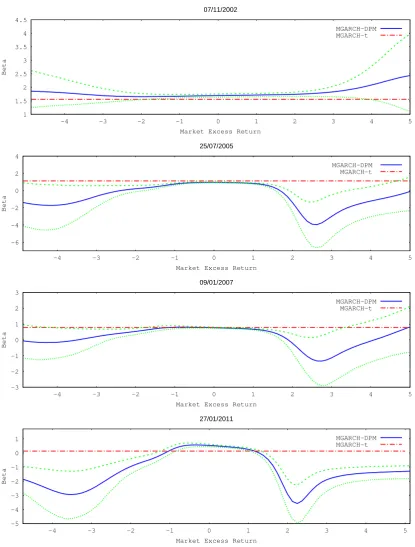
In Figure 14, generally returns outside of (−2,2) have density intervals that exclude the constant beta for the MGARCH-t. The deviation of the nonparametric beta from the constant one is very large for 27/01/2011. On the other hand, Figure 15 shows fewer episodes that differ from the constant beta for XOM. Figure 17 displays large deviations for 27/08/2003 and 23/10/2008 for AMGN and similarly for BAC 04/11/2011 (Figure 18). It is clear from these figures that there are significant departures of the nonparametric beta from the constant beta in the MGARCH-t model.

Finally, Figures 19-23 provide a three dimensional version of Figures 8-12 for each stock. In some periods beta is essentially flat and consistent with the MGARCH-t model while in other times beta is very sensitive to the market return.

8.1

Summary of Empirical Results

As the empirical results illustrate, the conditional beta is time-varying and at each time depends on the contemporaneous market excess return, as opposed to the constant beta of the benchmark model.

The previous results show some periods in which the conditional beta is insensitive to the value of rm,t (beta is almost constant with respect to rm,t) while in other time periods beta changes significantly with rm,t. To measure the sensitivity of bm,t(rm,t) to rm,t at each time t consider the following measure

dt= max

rm,t

bm,t(rm,t)−min

rm,t

bm,t(rm,t), (8.1)

where bm,t(rm,t) is defined in (5.10). Large values of dt indicate that bt(rm,t) is strongly

sensitive to r_m,t, while a dt = 0 indicates no sensitivity. The MGARCH-t model has a dt = 0 for all t. Figure 24 illustrates this dt over time for all individual stocks. Among these five stocks, the dynamic conditional beta for IBM and BAC have the most sensitivity and XOM has the least sensitivity tor_m,t. What is apparent is that during relatively high volatility periods such as 2002-03, 2009 and 2011:6-2012, dt attains its smallest values over the sample. In these periods shocks to the market are expected to be large. During lower volatility periods large shocks to the market and firms are unexpected and the conditional beta adjusts accordingly.

To investigate howbm,t(rm,t) changes with different market conditions Figures 25-29

show the broad trends that we find in all stocks. When the market is highly volatile, an individual stock’s conditional beta is less affected by unexpected shocks in the con-temporaneous market return. While in a calm market, the conditional beta changes remarkably from unexpected shocks to the market. However, the changes depend on the stocks correlation with the market.

It is often the case that the effect onbm,t(rm,t) fromrm,t is asymmetric. Frequently bm,t(rm,t) is more sensitive to large positive values of rm,t compared to negative values.

In addition, when the market is calm, we see both u-shape and inverse u-shape patterns for the conditional beta of all stocks.

9

Financial Applications

From Equation (5.5), we are able to examine the whole conditional density of the stock given factor values. This allows for the study of the individual stock’s conditional ex-pected return but also risk measures under different market scenarios. For instance, what is the expected return tomorrow of a stock if a market crash occurred or what is the value-at-risk in this case?

Consider the predictive conditional expected return of IBM at timet derived from the 1-factor model, E[rIBM,t|rm,1:t−1, rIBM,1:t−1]. Using the semiparametric model, this value is a nonlinear function of rm,t. Therefore, when a large shock is expected to the

market, this shock affects our expectation of the IBM return nonlinearly, while in the benchmark model this effect is linear. For instance, Figure 30 illustrates IBM’s predictive conditional expected return for a specific date (30/11/2000). From this figure we can assess the expected impact of a large positive or negative shock to the market on the value of IBM’s expected return.

Consider a second example of a large realized market shock in 29/10/2008 and the impact on IBM. Figure 31 shows IBM’s predictive conditional expected return for this day derived from the benchmark model and the semiparametric model. The realized market return and IBM return on this day are %9.77 and %9.56, respectively. Accounting for the nonlinearity using the semiparametric model reduces the prediction error considerably. The blue line from the nonparametric model is much closer to the realized return.

The previous example focused on one specific date. If we consider all dates in which the market had a large realized shock (more than 6%) the root mean squared error of

the prediction is reduced from 8.394 and 8.131 in moving from the MGARCH-t to the

nonparametric model. This represents a 3.2% improvement in accuracy.

In addition to the expected return, the semiparametric model enables us to study the effect of large shocks in the market on IBM’s whole conditional density and the impact on different risk measures. Figure 32 illustrates the effect of +5% and −5% shocks in the market return on IBM’s predictive conditional density on 17/05/2012. The value-at-risk from a $1 investment in IBM when we have no shock in the market is 2.306%. A +5% shock in the market return decreases the value-at-risk to 0.180%, while a −5% shock in the market return increases the value at risk to 4.471%. Therefore, we can carry out different risk scenario analyses in order to measure the effect of big shocks in the market on our investment in a specific firm.

10

Conclusion

return. In highly volatile markets, beta is almost constant, while in stable markets, the beta coefficient can depend asymmetrically on the contemporaneous value of the market excess return. The paper concludes with a discussion of how the model can be used to assess different risk scenarios.

11

Appendix

11.1

Distributions

If r∼t(µ,Σ, ν) then the density function of the Student-t (Bauwens et al. 2000) is

f(r|ν, µ,Σ) = Γ(

ν+p 2 )

Γ(ν₂)πp/2|Σ| −1/2

1 + 1

ν(r−µ)

T_Σ−1_(r−µ)

−(ν+p)/2

, ν >0.

The q×q matrix B follows an inverse Wishart density with a symmetric positive

definite scale matrix B0 and degree of freedomν0 ≥q+ 1, if its pdf can be written as

f(B|B0, ν0) = |B0|

ν0/2

2qν20π

q(q−1) 4 Πq

i=1Γ(ν0+1−i2 )

|B|−ν0+2q+1exp

−1

2tr(B

−1_B0)

,

with E(B) = 1

ν0−q−1B0.

The pdf of the Gamma distribution G(a, b) with shape parameter a and scale pa-rameter b is written as

f(x|a, b) = b

a

Γ(a)x

a−1_e−xb_{, x∈(0,∞), E(x) =} a b.

11.2

Derivation of the nonparametric conditional beta

E(ri,t|ri,t, r1:T, G(g)) =

K(g)

X

j=1

q_j(g)(rm,t)[µ(g)j,1 +β (g)

jt (rm,t−µ(g)j,2)]+ (11.1)

 1−

K(g)

X

j=1

q_j(g)(r_m,t)

  R

[µ1+βt(rm,t−µ2)]N(rm,t|µ2,(H(g)

1/2

t BH

(g)1/2′

t )22)p(µ, B)dµdB R

N(rm,t|µ2,(Ht(g)1/2BH (g)1/2′

t )22)p(µ, B)dµdB

.

Let

A1 =

Z

[µ1+βt(rm,t−µ2)]N(rm,t|µ2,(H(g)

1/2

t BH

(g)1/2′

t )22)p(µ, B)dµdB, (11.2)

A2 =

Z

N(rm,t|µ2,(H_t(g)1/2BH_t(g)1/2′)22)p(µ, B)dµdB. (11.3)

A1 and A2 can be easily approximated by Monte Carlo simulation as follows

A1 ≈ 1 N

N X

n=1

[µn,1+β_n,t(g)(rm,t −µn,2)]N(rm,t|µn,2,(H(g)

1/2

t BnH

(g)1/2′

t )22) (11.4)

A2 ≈ 1 N

N X

n=1

N(rm,t|µn,2,(H(g)

1/2

t BnH

(g)1/2′

where µn and Bn, n= 1, ..., N are i.i.d draws from the priorp(µ, B) which in our model

is N(µ|µ0, D) andW−1_{(B|B0, ν0), and}

β_nt(g)= (H

(g)1/2

t BnH

(g)1/2′

t )12

(Ht(g)1/2BnH (g)1/2′ t )22

. (11.6)

Now we obtain the posterior mean of the nonparametric conditional beta by taking the derivative of 11.1:

bm,t(rm,t) =

1

M M X

g=1

bm,t(rm,t, G(g)) =

1

M M X

g=1

∂E(ri,t|rm,t, r1:T, G(g)₎ ∂rm,t

rm,t=rm,t

. (11.7)

After replacing A1 and A2 with their approximations we have

∂E(ri,t|rm,t, r1:T, G(g))

∂rm,t ≈

K(g) X

j=1

q_j(g)(rm

t )β(jtg) (11.8)

+ K(g)

X

j=1

q′_j(g)(rtm)[µ(j,g1)+β (g)

jt (rtm−µ(j,g2))]

− K(g)

X

j=1

q′(g)

j (rtm) P

n[µn,1+βtn(g)(rmt −µn,2)]N(rmt |µn,2,(H(g)

1/2

t BnH(g)

1/2′

t )22)

P

nN(rmt |µn,2,(H(g)

1/2

t BnH(g)

1/2′

t )22)

+  1− K(g) X j=1

q(_jg)(rm t )



{ P

nβ

(g)

tnN(rtm|µn,2,(H(g)

1/2

t BnH(g)

1/2′

t )22)

P

nN(rmt |µn,2,(H(g)

1/2

t BnH(g)

1/2′

t )22)

+ P

n[µn,1+β(tng)(rtm−µn,2)]N′(rtm|µn,2,(H(g)

1/2

t BnH(g)

1/2′

t )22)

P

nN(rmt |µn,2,(H(g)

1/2

t BnH(g)

1/2′

t )22)

−[ P

n[µn,1+βtn(g)(rmt −µn,2)]N(rmt |µn,2,(H(g)

1/2

t BnH(g)

1/2′

t )22)]PnN′(rmt |µn,2,(H(g)

1/2

t BnH(g)

1/2′

t )22)

[P

nN(rmt |µn,2,(H(g)

1/2

t BnH(g)

1/2′

t )22)]2

}

whereβ_jt(g),β_nt(g), andq_j(g)(rm

t ) are defined in Equations (5.8), (11.6), and (5.6), respectively,

and N′_{(x|.) is the derivative of the pdf of Normal distribution with respect to x. In the}

case that we have more than one factor (say q factors), the derivations follow similarly but the derivative will be a vector of size q, each element of which is the coefficient of the corresponding factor.

References

Bauwens, L., Lubrano, M. & Richard, J.-F. (2000), Bayesian Inference in Dynamic

Econometric Models, Oxford University Press, Oxford.

Bollerslev, T., Engle, R. F. & Wooldridge, J. M. (1988), ‘A Capital Asset Pricing Model with Time-varying Covariances’,The Journal of Political Economy. 96(1), 116–131.

Choudhry, T. (2002), ‘The Stochastic Structure of the Time-Varying Beta: Evidence

from UK Companies’,The Manchester School 70(6), 768–791.

Engle, R. F. (2016), ‘Dynamic conditional beta’, Journal of Financial Econometrics

14(4), 643–667.

Engle, R. F. & Ng, V. K. (1993), ‘Measuring and Testing the Impact of News on Volatil-ity’, The Journal of Finance48(5), 1749–1778.

Escobar, M. D. & West, M. (1995), ‘Bayesian Density Estimation and Inference using Mixtures’, Journal of the American Statistical Association 90(430), 577–588.

Fama, E. F. & French, K. R. (1993), ‘Common Risk Factors in the Returns on Stocks and Bonds’,Journal of Financial Economics 33(1), 3–56.

Ferguson, T. S. (1973), ‘A Bayesian Analysis of Some Nonparametric Problems’, The

Annals of Statistics 1, 209–230.

Giannopoulos, K. (1995), ‘Estimating the Time-varying Components of International Stock Markets Risk’,European Journal of Finance 1(2), 129–164.

Jensen, M. J. & Maheu, J. M. (2013), ‘Bayesian Semiparametric Multivariate GARCH Modeling’,Journal of Econometrics 176(1), 3–17.

Kalli, M., Griffin, J. E. & Walker, S. G. (2011), ‘Slice Sampling Mixture Models’,Statistics and Computing 21(1), 93–105.

Lintner, J. (1965), ‘The Valuation of Risk Assets and the Selection of Risky Investments

in Stock Portfolios and Capital Budgets’, The Review of Economics and Statistics

47(1), 13–37.

Lo, A. Y. (1984), ‘On a Class of Bayesian Nonparametric Estimates: I. Density Esti-mates.’,The Annals of Statistics 12(1), 351–357.

McCurdy, T. H. & Morgan, I. (1992), ‘Evidence of Risk Premiums in Foreign Currency Futures Markets’,Review of Financial Studies 5(1), 65–83.

Roth, M. (2013), On the Multivariate t Distribution, Technical Report 3059. http://www.diva-portal.org/smash/get/diva2:618567/FULLTEXT02.

Sethuraman, J. (1994), ‘A Constructive Definition of Dirichlet Priors.’, Statistica Sinica

4, 639–650.

Sharpe, W. F. (1964), ‘Capital Asset Prices: A Theory of Market Equilibrium under Conditions of Risk’,The Journal of Finance 19(3), 425–431.

Walker, S. G. (2007), ‘Sampling the Dirichlet Mixture Model with Slices’,

Stock Mean Variance Skewness Kurtosis Max Min

Market 0.017 1.744 -0.070 7.067 11.350 -8.950

IBM 0.028 3.070 0.230 7.834 13.019 -15.567

GE -0.003 4.277 0.323 8.397 19.702 -12.797

XOM 0.032 2.672 0.367 11.163 17.180 -13.950

AMGN 0.034 4.758 0.508 5.907 15.090 -13.437

BAC 0.031 10.701 0.891 23.399 35.261 -28.969

Table 1: Summary statistics of the daily excess returns on the market portfolio, IBM, GE, XOM and AMGN, BAC from 03/01/2000 to 31/12/2013 (3521 observations).

Log Marginal Predictive Likelihood

Stock 1-factor model 3-factor model 4-factor model

IBM −774.37 −1017.72 −1240.97

AMGN −917.05 −1200.30 −1347.57

BAC −1071.36 −1235.12 −1451.62

XOM −671.59 −889.56 −1074.24

GE −774.43 −970.31 −1123.54

Table 2: This table reports the marginal log-predictive likelihood for MGARCH-DPM model, for the last 500 observations, from 12/03/2012 to 31/12/2013 for the univariate stock return. Data are daily excess market returns, SMB, HML and momentum returns coupled with excess returns on IBM, AMGN, BAC, XOM and GE from 03/01/2000 to 31/12/2013. The 1-factor model includes the market, the 3-factor model the market, SMB and HML, the 4-factor model the market, SMB, HML and momentum

log-predictive likelihood

Model IBM GE XOM AMGN BAC

MGARCH-DPM −983.27 −964.99 −875.47 −1140.12 −1473.11

MGARCH-t −1353.67 −1369.03 −1300.21 −1571.32 −1684.72

log-Bayes factor 370.40 404.04 424.74 431.20 211.61

IBM MGARCH-DPM MGARCH-t

Parameter Post. Mean 95% DI Post. Mean 95% DI

γ01 0.102 (0.055,0.146) 0.023 (0.015,0.037)

γ02 −0.043 (−0.081,0.003) −0.042 (−0.053,−0.034)

γ03 0.020 (0.001,0.053) 0.020 (0.002,0.048)

γ11 0.247 (0.199,0.307) 0.150 (0.144,0.160)

γ12 0.267 (0.232,0.313) 0.224 (0.210,0.233)

γ21 0.971 (0.965,0.977) 0.975 (0.971,0.977)

γ22 0.953 (0.945,0.961) 0.955 (0.951,0.961)

µ1 0.025 (0.016,0.046)

µ2 0.041 (0.022,0.074)

ν 5.37 (5.01,5.54)

c 5.6 (3.00,11.0)

α 0.571 (0.070,1.61)

η1 0.570 (0.349,0.714) 0.807 (0.776,0.864)

η2 0.533 (0.434,0.618) 0.507 (0.451,0.644)

Table 4: IBM Estimates: This table displays posterior mean and 95% density intervals (DI) for the parameters of MGARCH-DPM and MGARCH-t models. Data is daily excess returns on IBM and excess market returns. Data is from Jan 3, 2000 to Dec 31, 2013 (3521 observations).

XOM MGARCH-DPM MGARCH-t

Parameter Post. Mean 95% DI Post. Mean 95% DI

γ01 0.141 (0.108,0.182) 0.110 (0.012,0.200)

γ02 0.014 (−.003,0.030) 0.016 (−0.058,0.073) γ03 0.014 (0.001,0.041) 0.032 (0.001,0.082)

γ11 0.250 (0.223,0.283) 0.228 (0.165,0.310)

γ12 0.238 (0.198,0.287) 0.228 (0.175,0.288) γ21 0.956 (0.947,0.965) 0.958 (0.935,0.977)

γ22 0.960 (0.953,0.969) 0.958 (0.939,0.974)

µ1 0.025 (−0.076,0.129)

µ2 0.022 (−0.050,0.092)

ν 9.89 (6.16,13.90)

c 3.6 (2.00,9.00)

α 0.324 (0.011,1.15)

η1 0.480 (0.345,0.591) 0.436 (−0.051,0.775)

η2 0.524 (0.436,0.613) 0.514 (0.279,0.708)

GE MGARCH-DPM MGARCH-t

Parameter Post. Mean 95% DI Post. Mean 95% DI

γ01 0.061 (0.023,0.093) 0.031 (0.012,0.056)

γ02 −0.033 (−0.054,−0.014) −0.029 (−0.039,−0.008)

γ03 0.018 (0.001,0.052) 0.036 (0.022,0.052)

γ11 0.196 (0.174,0.216) 0.170 (0.145,0.188)

γ12 0.204 (0.181,0.225) 0.180 (0.168,0.192)

γ21 0.974 (0.967,0.981) 0.974 (0.970,0.981)

γ22 0.964 (0.957,0.970) 0.971 (0.967,0.974)

µ1 0.004 (−0.034,0.029)

µ2 0.049 (0.015,0.071)

ν 6.47 (5.35,7.05)

c 5.04 (3.00,10.0)

α 0.501 (0.060,1.42)

η1 0.554 (0.414,0.707) 0.633 (0.555,0.785)

η2 0.464 (0.395,0.539) 0.463 (0.416,0.561)

Table 6: GE Estimates: This table displays posterior mean and 95% density intervals (DI) for the parameters of MGARCH-DPM and MGARCH-t models. Data is daily excess returns on GE and excess market returns. Data is from Jan 3, 2000 to Dec 31, 2013 (3521 observations).

AMGN MGARCH-DPM MGARCH-t

Parameter Post. Mean 95% DI Post. Mean 95% DI

γ01 0.137 (0.089,0.171) 0.084 (0.065,0.106)

γ02 −0.011 (−0.031,0.012) −0.028 (−0.044,−0.007) γ03 0.016 (0.001,0.039) 0.034 (0.015,0.059)

γ11 0.211 (0.182,0.239) 0.165 (0.156,0.175)

γ12 0.188 (0.172,0.211) 0.228 (0.195,0.242) γ21 0.965 (0.945,0.958) 0.973 (0.971,0.976)

γ22 0.951 (0.945,0.958) 0.956 (0.950,0.965)

µ1 0.002 (−0.014,0.035)

µ2 0.038 (0.024,0.070)

ν 5.81 (5.56,6.08)

c 15 (7.00,28.0)

α 2.41 (0.500,5.21)

η1 0.508 (0.428,0.596) 0.768 (0.686,0.876)

η2 0.542 (0.459,0.630) 0.479 (0.443,0.566)

BAC MGARCH-DPM MGARCH-t

Parameter Post. Mean 95% DI Post. Mean 95% DI

γ01 0.064 (0.024,0.115) 0.065 (0.045,0.091) γ02 −0.031 (−0.062,0.012) −0.022 (−0.036,−0.008)

γ03 −0.007 (−0.061,0.042) 0.029 (0.004,0.051)

γ11 0.284 (0.235,0.351) 0.219 (0.206,0.238) γ12 0.212 (0.183,0.260) 0.213 (0.197,0.229)

γ21 0.962 (0.954,0.968) 0.962 (0.956,0.966)

γ22 0.955 (0.945,0.963) 0.963 (0.956,0.969)

µ1 0.000 (−0.033,0.033)

µ2 0.040 (0.021,0.072)

ν 6.37 (5.992,6.839)

c 6.24 (3.000,12.000)

α 0.658 (0.092,1.800)

η1 0.436 (0.326,0.547) 0.472 (0.400,0.554)

η2 0.414 (0.333,0.501) 0.432 (0.354,0.558)

-30 -20 -10 0 10 20 30 40

2000 2001 2002 2003 2004 2005 2006 2007 2008 2009 2010 2011 2012 2013 2014

BAC -15

-10 -5 0 5 10 15 20

2000 2001 2002 2003 2004 2005 2006 2007 2008 2009 2010 2011 2012 2013 2014

AMGN -15

-10 -5 0 5 10 15 20

2000 2001 2002 2003 2004 2005 2006 2007 2008 2009 2010 2011 2012 2013 2014

XOM -15

-10 -5 0 5 10 15 20

2000 2001 2002 2003 2004 2005 2006 2007 2008 2009 2010 2011 2012 2013 2014

GE -20

-15 -10 -5 0 5 10 15

2000 2001 2002 2003 2004 2005 2006 2007 2008 2009 2010 2011 2012 2013 2014

IBM -10

-5 0 5 10 15

2000 2001 2002 2003 2004 2005 2006 2007 2008 2009 2010 2011 2012 2013 2014

Market

-2 0 2 4 6 8 10 12 14

12-Feb 12-Apr 12-Jun 12-Aug 12-Oct 12-Dec 13-Feb 13-Apr 13-Jun 13-Aug 13-Oct 13-Dec

Difference in Log-predictive Likelihoods

t

-10 -8 -6 -4 -2 0 2 4 6

12-Feb 12-Apr 12-Jun 12-Aug 12-Oct 12-Dec 13-Feb 13-Apr 13-Jun 13-Aug 13-Oct 13-Dec

IBM Excess Return

t

-3 -2 -1 0 1 2 3

12-Feb 12-Apr 12-Jun 12-Aug 12-Oct 12-Dec 13-Feb 13-Apr 13-Jun 13-Aug 13-Oct 13-Dec

Market Excess Return

t

-1 -0.5 0 0.5 1 1.5 2

2000 2001 2002 2003 2004 2005 2006 2007 2008 2009 2010 2011 2012 2013 2014

Beta

t

MGARCH-t MGARCH-DPM

Figure 3: IBM: Realized conditional beta over time from MGARCH-t and MGARCH-DPM models.

-1 -0.5 0 0.5 1 1.5 2

2000 2001 2002 2003 2004 2005 2006 2007 2008 2009 2010 2011 2012 2013 2014

Beta

t

MGARCH-t MGARCH-DPM

Figure 4: XOM: Realized conditional beta over time from MGARCH-t and MGARCH-DPM models.

0 0.5 1 1.5 2 2.5

2000 2001 2002 2003 2004 2005 2006 2007 2008 2009 2010 2011 2012 2013 2014

Beta

t

MGARCH-t MGARCH-DPM

-1 -0.5 0 0.5 1 1.5 2 2.5 3

2000 2001 2002 2003 2004 2005 2006 2007 2008 2009 2010 2011 2012 2013 2014

Beta

t

MGARCH-t MGARCH-DPM

Figure 6: AMGN: Realized conditional beta over time from MGARCH-t and MGARCH-DPM models.

0 0.5 1 1.5 2 2.5 3 3.5 4 4.5 5 5.5

2000 2001 2002 2003 2004 2005 2006 2007 2008 2009 2010 2011 2012 2013 2014

Beta

t

MGARCH-t MGARCH-DPM

Figure 7: BAC: Realized conditional beta over time from MGARCH-t and MGARCH-DPM models.

-7 -6 -5 -4 -3 -2 -1 0 1 2

-6 -4 -2 0 2 4

Beta

Market Excess Return 30/11/2000

30/10/2013 14/05/2003 06/10/2006 26/08/2009

18/10/2012

-2 -1.5 -1 -0.5 0 0.5 1 1.5 2 2.5

-6 -4 -2 0 2 4

Beta

Market Excess Return

08/02/2007 28/11/2001

01/09/2006 22/11/2006

17/02/2005

Figure 9: XOM: posterior mean of conditional beta as a function of the market excess return for different dates.

-2 -1.5 -1 -0.5 0 0.5 1 1.5 2 2.5 3

-6 -4 -2 0 2 4

Beta

Market Excess Return

18/09/2009

28/11/2012

08/01/2004 16/02/2011 06/09/2000 19/12/2006

-1 0 1 2 3 4 5 6 7 8

-6 -4 -2 0 2 4

Beta

Market Excess Return

21/05/2002 21/05/2001

22/03/2004 23/02/2005

07/02/2007

27/09/2012

-5 -4 -3 -2 -1 0 1 2 3 4

-6 -4 -2 0 2 4

Beta

Market Excess Return

09/05/2012 22/10/2013

28/12/2012

23/01/2013 28/04/2011

08/04/2010

Figure 12: BAC: posterior mean of conditional beta as a function of the market excess return for different dates.

-10 -8 -6 -4 -2 0 2 4 6

-6 -4 -2 0 2 4

E(r

t

IBM

|r

t

m)

Market Excess Return 30/11/2000

30/10/2013

14/05/2003 06/10/2006 26/08/2009 18/10/2012

1 1.5 2 2.5 3 3.5 4 4.5

-4 -3 -2 -1 0 1 2 3 4 5

Beta

Market Excess Return 07/11/2002

MGARCH-DPM MGARCH-t

-6 -4 -2 0 2 4

-4 -3 -2 -1 0 1 2 3 4 5

Beta

Market Excess Return 25/07/2005

MGARCH-DPM MGARCH-t

-3 -2 -1 0 1 2 3

-4 -3 -2 -1 0 1 2 3 4 5

Beta

Market Excess Return 09/01/2007

MGARCH-DPM MGARCH-t

-5 -4 -3 -2 -1 0 1

-4 -3 -2 -1 0 1 2 3 4 5

Beta

Market Excess Return 27/01/2011

MGARCH-DPM MGARCH-t

0.2 0.4 0.6 0.8 1 1.2

-4 -3 -2 -1 0 1 2 3 4 5

Beta

Market Excess Return 29/04/2010

MGARCH-DPM MGARCH-t -2

-1 0 1 2 3

-4 -3 -2 -1 0 1 2 3 4 5

Beta

Market Excess Return 03/03/2005

MGARCH-DPM MGARCH-t

0.6 0.8 1 1.2 1.4 1.6 1.8 2 2.2 2.4

-4 -3 -2 -1 0 1 2 3 4 5

Beta

Market Excess Return 25/04/2011

MGARCH-DPM MGARCH-t 0.5

1 1.5 2 2.5 3 3.5

-4 -3 -2 -1 0 1 2 3 4 5

Beta

Market Excess Return 09/01/2006

MGARCH-DPM MGARCH-t

-3 -2 -1 0 1

-4 -3 -2 -1 0 1 2 3 4 5

Beta

Market Excess Return 28/09/2000

MGARCH-DPM MGARCH-t

1 1.5 2 2.5 3 3.5

-4 -3 -2 -1 0 1 2 3 4 5

Beta

Market Excess Return 31/12/2002

MGARCH-DPM MGARCH-t

-2 -1.5 -1 -0.5 0 0.5 1 1.5

-4 -3 -2 -1 0 1 2 3 4 5

Beta

Market Excess Return 16/07/2004

MGARCH-DPM MGARCH-t

-2 -1.5 -1 -0.5 0 0.5 1 1.5 2

-4 -3 -2 -1 0 1 2 3 4 5

Beta

Market Excess Return 10/01/2011

MGARCH-DPM MGARCH-t

0.75 0.8 0.85 0.9 0.95 1 1.05

-4 -3 -2 -1 0 1 2 3 4 5

Beta

Market Excess Return 23/10/2008

MGARCH-DPM MGARCH-t

-3 -2 -1 0 1 2

-4 -3 -2 -1 0 1 2 3 4 5

Beta

Market Excess Return 08/10/2012

MGARCH-DPM MGARCH-t 0

2 4 6 8 10 12 14

-4 -3 -2 -1 0 1 2 3 4 5

Beta

Market Excess Return 27/08/2003

MGARCH-DPM MGARCH-t

-1 0 1 2 3

-4 -3 -2 -1 0 1 2 3 4 5

Beta

Market Excess Return 31/05/2005

MGARCH-DPM MGARCH-t

1.5 2 2.5 3 3.5 4 4.5

-5 -4 -3 -2 -1 0 1 2 3 4 5

Beta

Market Excess Return 18/01/2012

MGARCH-DPM MGARCH-t

-10 -8 -6 -4 -2 0 2 4

-5 -4 -3 -2 -1 0 1 2 3 4 5

Beta

Market Excess Return 19/03/2013

MGARCH-DPM MGARCH-t 0.4

0.6 0.8 1 1.2 1.4 1.6 1.8 2

-5 -4 -3 -2 -1 0 1 2 3 4 5

Beta

Market Excess Return 24/05/2012

MGARCH-DPM MGARCH-t 2.2

2.4 2.6 2.8 3 3.2 3.4

-5 -4 -3 -2 -1 0 1 2 3 4 5

Beta

Market Excess Return 04/11/2011

MGARCH-DPM MGARCH-t

Figure 19: The posterior mean of IBM’s nonparametric conditional beta as a function of excess market return and time from 2009-07 to 2010-03 estimated with MGARCH-DPM model.

Figure 21: The posterior mean of GE’s nonparametric conditional beta as a function of excess market return and time from 2009-12 to 2010-06 estimated with MGARCH-DPM model.

Figure 23: The posterior mean of BAC’s nonparametric conditional beta as a function of excess market return and time from 2012-10 to 2013-04 estimated with MGARCH-DPM model.

0 1 2 3 4 5 6 7 8 9 10

2000 2001 2002 2003 2004 2005 2006 2007 2008 2009 2010 2011 2012 2013 2014

dt

t

IBM XOM GE AMGN BAC

Figure 24: Variability of conditional beta with respect to the contemporaneous value of market excess returns over time for different stocks. dt= max

rm,t

bm,t(rm,t)−min

rm,t

0.4 0.5 0.6 0.7 0.8 0.9 1 1.1 1.2

-4 -2 0 2 4

Beta

Market Excess Return Highly volatile market

-4 -3 -2 -1 0 1 2

-4 -2 0 2 4

Beta

Market Excess Return

Calm market, when correlation between market and IBM is low

0.8 1 1.2 1.4 1.6 1.8 2 2.2

-4 -2 0 2 4

Beta

Market Excess Return

Calm market, when correlation between market and IBM is high

0.6 0.7 0.8 0.9 1 1.1 1.2 1.3 1.4

-4 -2 0 2 4

Beta

Market Excess Return Highly volatile market

-1 -0.5 0 0.5 1 1.5

-4 -2 0 2 4

Beta

Market Excess Return

Calm market, when correlation between market and XOM is low

0.8 1 1.2 1.4 1.6 1.8 2 2.2 2.4

-4 -2 0 2 4

Beta

Market Excess Return

Calm market, when correlation between market and XOM is high

-0.8 -0.6 -0.4 -0.2 0 0.2 0.4 0.6 0.8 1 1.2

-4 -2 0 2 4

Beta

Market Excess Return

Calm market, when correlation between market and GE is low

1 1.2 1.4 1.6 1.8 2 2.2

-4 -2 0 2 4

Beta

Market Excess Return

Calm market, when correlation between market and GE is high 0.6

0.7 0.8 0.9 1 1.1 1.2 1.3 1.4 1.5

-4 -2 0 2 4

Beta

Market Excess Return Highly volatile market

0.4 0.5 0.6 0.7 0.8 0.9 1

-4 -2 0 2 4

Beta

Market Excess Return Highly volatile market

-1.5 -1 -0.5 0 0.5 1 1.5

-4 -2 0 2 4

Beta

Market Excess Return

Calm market, when correlation between market and AMGN is low

0 1 2 3 4 5 6

-4 -2 0 2 4

Beta

Market Excess Return

Calm market, when correlation between market and AMGN is high

0.8 1 1.2 1.4 1.6 1.8 2 2.2 2.4 2.6 2.8

-4 -2 0 2 4

Beta

Market Excess Return Highly volatile market

-7 -6 -5 -4 -3 -2 -1 0 1 2

-4 -2 0 2 4

Beta

Market Excess Return

Calm market, when correlation between market and BAC is low

1 2 3 4 5 6 7 8

-4 -2 0 2 4

Beta

Market Excess Return

Calm market, when correlation between market and BAC is high

-4 -3 -2 -1 0 1 2 3 4

-4 -2 0 2 4

E(r

t

IBM

|r

t

m, r

1:t-1

)

Market Excess Return

30/11/2000

DPM-GARCH GARCH-t

Figure 30: IBM: Predictive conditional expected return of IBM derived from MGARCH-DPM and MGARCH-t model.

-10 -8 -6 -4 -2 0 2 4 6 8 10

-10 -5 0 5 10

E(r

t

IBM

|r

t

m, r

1:t-1

)

Market Excess Return 28/10/2008

DPM-GARCH GARCH-t Realized

0 0.1 0.2 0.3 0.4 0.5 0.6 0.7

-6 -4 -2 0 2 4

Conditional Density

IBM Excess return 17/05/2012

+5% shock in the market -5% shock in the market No shock in the market