A Study on Using Multiple Sets of Particle Filters to Control an Inverted Pendulum

(1)

A Study on Using Multiple Sets of Particle Filters

to Control an Inverted Pendulum

Midori Saito and Ichiro Kobayashi

Abstract—The dynamic system is controlled by various ap-proaches by means of the equation of motion which approxi-mates its motion characteristics with a linear function. There is however much noise in the real control environment. So, we often encounter the situation in which we cannot completely ap-proximate such non-linear states in a target system with a linear function. In recent years, the particle filter is often used for the prediction of non-linear states of a system and for controlling the system. In this paper, we propose a method which predicts not directly observable control variable through sharing the likelihood of an observable variable by means of multiple sets of particle filters. We employ an inverted pendulum as the target system to be controlled; examine the ability of our proposed method from views of stability and robustness; and show the method has both strong characteristics.

Index Terms—particle filters, inverted pendulum, likelihood sharing

I. INTRODUCTION

T

HE system is controlled by various approaches using the equation of motion. There is however much noise in the real control environment. So, we often encounter the cases where we may not be able to completely approximate such non-linear states with an equation of motion. The particle filter is a method to estimate the states of a system by means of a probabilistic distribution, and recently it has been widely used in system control [1], [2], [3]. The inverted pendulum includes non-linear states to control itself and the control mechanism itself is simple, so it is often used to testify various proposed methods to control a system including non-linear characteristics in itself [1], [4], [5]. In this study, we aim to propose a control method using particle filters to estimate not directly observable states of a system and control the system. As a target system to be controlled in this paper, we employ an inverted pendulum and estimate the force given to the cart of the pendulum, which cannot be directly observed, through an observable variable — here, the angle of pendulum from its standing position. Moreover, we show our proposed method has strong robustness for the disturbances in the control environment.

II. RELATED STUDIES

In general, in order to control a non-linear system, the method using non-linear feedback or linear approximation based on the first approximation of Taylor developing is widely used, however, there are cases where some systems cannot be controlled because of their strong non-linearity. To overcome the problem with non-linearity, Yamada et al. [6] proposed a method to combine the non-linear feedback and coordination transformation, they were successful in making

M. Saito and I. Kobayashi are with Advanced Sciences, Graduate School of Humanities and Sciences, Ochanomizu University, Tokyo, Japan e-mail: {saito.midori,koba}@is.ocha.ac.jp

an inverted pendulum stand upright from the vertical below position on a simulator. Furthermore, Inoue et al. [4], [5] employed fuzzy rules which controls an inverted pendulum, automatically generated by a genetic algorithm, taking ac-count of the symmetrical movement of an inverted pendulum. However, as for the control of an inverted pendulum which requires more non-linear control in the real environments where many disturbances exist, since the former study pro-poses a linearization method, so the strict stability is not guaranteed by the study. Moreover, the latter study needs to design new fuzzy rules to respond to disturbances. So, in general, if the target system to be controlled contains disturbances in its characteristics, we had better introduce non-linear control to the system. In this context, Kashimura et al. [7] have introduced particle filter into the framework for reinforcement learning to select a relevant policy based on representing experience on action with probabilistic dis-tribution. Although introducing particle filter into non-linear control is related to our approach, in the case of the control in a real environment, to build a probabilistic distribution with particle filter for each estimated state and provide reward to the states might become a big problem in terms of processing cost. Sun et al. [2] constructed a controller for an inverted pendulum with a neural network and employed particle filter to estimate its parameters. Furthermore, they have compared the control effect between Kalman filter and particle filter and then shown that particle filter improves markedly than Kalman filter both on speed and precision. Stahl et al. [3] proposed a method to control an inverted pendulum by introducing two nest particle filters, introducing the idea of model predictive control into stochastic nonlinear systems.

In this study, we introduce multiple sets of particle fil-ters for estimating an unobservable controlled variable of a system from an observable variable through sharing the likelihood of the particles representing those non-linear states of the system, and then propose a method of a robust control against disturbances existing in the environment. Moreover, through simulation experiments we compare the abilities between the control which approximates the continuous space with a linear equation of motion and the control we propose.

III. PARTICLE FILTER

The particle filter is a time-series filter which does not have any constraint on the shape of probabilistic mass function to estimate the states of a system, it can therefore estimate the states of a non-linear system. Particle filters estimate an unobservable statextwith an observable stateyt. Both states

(2)

xt = Ftxt₋1+Gtvt (1)

yt = Htxt+wt (2)

In (1) and (2),vtandwtindicate system noise and observed noise, respectively.Ft，Gt，Htindicate coefficient matrices corresponding to each variable. The state xt is represented

with a set ofK weighted particles,Xt={(x

(k)

t , π

(k)

t )} K

k=1,

whereπt(k) indicates the weight of each particle.

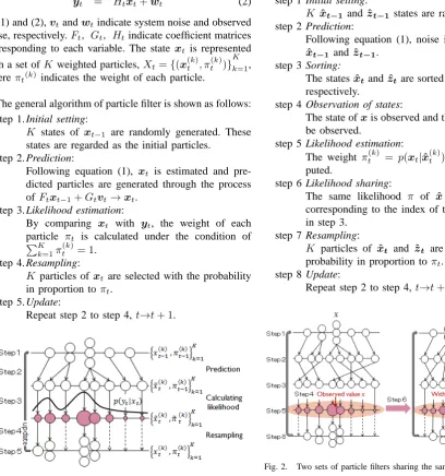
The general algorithm of particle filter is shown as follows: step 1. Initial setting:

K states of xt₋1 are randomly generated. These

states are regarded as the initial particles. step 2. Prediction:

Following equation (1), xt is estimated and pre-dicted particles are generated through the process of Ftxt−1+Gtvt→xt.

step 3. Likelihood estimation:

By comparing xt with yt, the weight of each particle πt is calculated under the condition of ∑K

k=1π (k)

t = 1. step 4. Resampling:

K particles of xtare selected with the probability in proportion toπt.

step 5. Update:

[image:2.595.61.470.98.535.2]

Repeat step 2 to step 4, t→t+ 1.

Fig. 1. Process of particle filters

As shown in Figure 1, a series of process: prediction, likelihood estimation, resampling, and update are repeated. By this, the state yt is tracked by multiple particles Xt.

IV. LIKELIHOOD SHARING FOR STATE ESTIMATION

In the control of an inverted pendulum, we assume that there is dependency between the deflection of pendulum and the other control variables corresponding to the deflection, for example, the force necessary given to the cart of the pendulum to make an inverted pendulum stand upright. The force is not observed directly but can be estimated by an observable state, i.e., the angle of the pendulum from its upright position. In general, particle filters can only track observable states, whereas our proposed method can estimate unobservable states by employing the architecture of sharing likelihood through multiple sets of particle filters.

In this study, we employ two sets of particle filters as

ex-pressed inXt={xˆ

(k)

t ,zˆ

(k)

t , π

(k)

t } K

k=1, then an unobservable

state z is estimated from an observable state x, in the case that there is dependency betweenxandz.

The algorithm of the proposed method is shown as follows: step 1 Initial setting:

K ˆxt−1 andˆzt−1states are randomly generated. step 2 Prediction:

Following equation (1), noise is provided to both

ˆ

xt−1 andˆzt−1. step 3 Sorting:

The statesxˆt andzˆt are sorted in ascending order, respectively.

step 4 Observation of states:

The state ofxis observed and the state ofz cannot be observed.

step 5 Likelihood estimation: The weight πt(k) = p(xt|xˆ

(k)

t )(1≤k≤K) is com-puted.

step 6 Likelihood sharing:

The same likelihood π of xˆ is provided to zˆ, corresponding to the index of the result of sorting in step 3.

step 7 Resampling:

K particles of xˆt and ˆzt are extracted with the probability in proportion toπt.

step 8 Update:

Repeat step 2 to step 4,t→t+ 1.

Fig. 2. Two sets of particle filters sharing the same likelihood

In step 1 and step 2, the same process of normal particle filters is performed. In step 3, the particles of xˆ and zˆ

are sorted in ascending order, since they were randomly generated at step 1. Here, by sorting the particles,πtwill be able to be shared as the weight ofzîn relation to the index ofxât step 6. As for bothxândzˆ, the processes after step 7 are the same as those of the normal particle filter. Like this, by sharing likelihood using two sets of particle filters, the unobservable state ofz will be able to estimate from the observable state ofx.

V. EXPERIMENT: STABILIZING CONTROL OF AN INVERTED PENDULUM

We conduct experiments with an inverted pendulum to confirm the control ability of our proposed method by comparing the control method using the equation of motion.

A. Experimental settings

(3)

to control, referring to [3]. The inverted pendulum consists of the upper and lower parts, i.e., pendulum and cart. Here, the length and the mass of the pendulum are l = 0.5(m) and m = 0.3(kg). The mass of cart is mc = 3.0(kg), respectively. The angle of pendulum from the upright po-sition is ϕ(rad), and angular acceleration is ϕ¨(rad/s2_).

Moving distance, speed and acceleration of the cart arep(m), ˙

p(m/s), p¨(m/s2), respectively. The acceleration of gravity

[image:3.595.355.508.218.278.2]

g is 9.8(m/s2). We use a physics engine called PhysX [8]. PhysX can perform on-line calculation of the physical characteristics of an object and illustrates the state of the object simultaneously. We use it to simulate the physical characteristics of a pendulum represented with the equation of motion and with our proposed model.

Fig. 3. Overview of the inverted pendulum

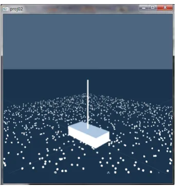
[image:3.595.58.281.243.334.2]

Figure 4 illustrates an example of simulation environment. The white and small objects scattered under the cart are disturbances to the cart.

Fig. 4. Simulation environment on PhysX (with disturbances)

The specification of the computer we have used for sim-ulation is shown in Table I.

TABLE I

THE SPECIFICATION OFPCUSED IN THE EXPERIMENTS

Item Specification

CPU Intel Core2 Duo P8800 (2.66GHz 2.67GHz)

RAM 4GByte

Graphics Mobile Intel 4 Series Express Chipset

B. Equation of motion for an inverted pendulum

If the goal of controlling an inverted pendulum is to make it stand upright, it is reported that we can regard an

inverted pendulum as symmetrical system around the upright position [4]. In this study, we also use this characteristics to achieve stabilizing the pendulum in the condition of standing upright. Considering such motion characteristics of a pendulum around the upright position, we think that the control needs less calculation rather than the other cases.

C. Control with the equation of motion

The equation of motion of an inverted pendulum is ex-pressed with the following equation defined in [3].

¨

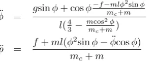
ϕ = gsinϕ+ cosϕ

−f₋mlϕ2_sin_ϕ

mc+m

l(4₃−m_mcos2ϕ

c+m)

(3)

¨

p = f+ml(ϕ

2_sin_ϕ₋_ϕ¨_cos_ϕ₎

mc+m

(4)

Here, we approximate the motion of the inverted pendulum around the upright position, i.e., (ϕ = 0,2π,ϕ˙ = 0), with the following equation.

f1(ϕ) = −0.806314ϕ2+ 5.06622ϕ (5)

The equation of f1 is approximated with the quadratic equation of ϕas expressed in (5) defined in [3]. Therefore, we setϕas the control target and regard it as the controlled variable given to the cart by transforming ϕ to f through equation (5). Moreover, we control the pendulum aroundϕ= 0 with equation (5) under the following 4 conditions of the position and the angular acceleration of the pendulum.

f(ϕ) =       

−f1(ϕ) if(p >0,ϕ >˙ 0)

f1(−ϕ) if(p >0,ϕ <˙ 0)

f1(ϕ) if(p≤0,ϕ >˙ 0) −f1(−ϕ) if(p≤0,ϕ <˙ 0)

(6)

D. State estimation by sharing likelihood

Even though the inverted pendulum is effected by dis-turbances, the controlled variablef depends on ϕ, i.e., the angle from upright position. In this study, we prepare 500 particles to estimate the angle ϕ and the force f provided to the cart — two sets of particle filters are expressed as

Xt={ϕˆ

(k)

t ,fˆ

(k)

t , π

(k)

t } K

k=1.fis usually obtained from given ϕ through the equation (5), however, by using proposed method, the unobservable variable fˆ is estimated by the observable variableϕ.

For estimation, the range of the initial values ofϕˆandfˆ

are set as follows:

0.0 ≤ {ϕˆ₀(k)}K_k₌₁ ≤0.5 (7)

0.0≤ {fˆ₀(k)}K_k₌₁ ≤10.0 (8)

[image:3.595.86.254.411.590.2]

(4)

into two cases: i.e., positive and negative, depending on the direction of deflection of the inverted pendulum.

f = {

rfˆ if (p <0.0)

−rfˆ if (p≥0.0) (9)

The initial values ofϕˆandfˆmentioned above are empir-ically decided, and also we have set the range of those as follows:0.0≤ϕ0ˆ ≤0.5,0.0≤f0ˆ ≤10.0,r= 5.0.

Moreover, in order to decide the number of particles to estimate the angle ϕ and the force f given to the cart of the pendulum, we compared the cases where the number of particles is 50, 100, and 500. Figure 5 shows the average of 5 trials of the error between estimate angleϕˆand the real angle

[image:4.595.338.505.53.152.2]

ϕ – the horizontal axis indicates time steps and the vertical axis indicates error from the real angle. As a result, we confirmed that the accuracy gets increased as the number of particles increased. Based on this result, in this experiment, we use 500 particles taking account of the graphic speed of the physical engine, PhysX.

Fig. 5. Relation between number of particles and error from the real value

E. Experimental results and discussions

Control with the equation of motion: Figure 6 and Figure

7 show the results of the cases where there is not any disturbance in the environment. Figure 8 and Figure 9 show the results of the cases where there is disturbance in the environment. Moreover, Figure 6 and Figure 8 show the absolute value of the angle of the inverted pendulum ϕ

when the equation of its motion is approximately expressed with a linear function. Figure 7 and Figure 9 show the position of the center of gravity of the inverted pendulum from a viewpoint of the fulcrum of the pendulum. We see from Figures 8 and 9 that the controller which had been able to control the pendulum with the equation of motion became unable to control in the environment with lots of disturbances.

In the case that disturbances were provided in the environ-ment, at the initial stage of controlling the pendulum, it could be controlled, but the control error given by the disturbances had been getting accumulated as time passed, and finally the pendulum had become unable to be controlled and was fallen down (see, Figures 8 and 9).

[image:4.595.350.509.194.292.2]

Fig. 6. Angleϕ(without disturbances)

[image:4.595.59.278.316.445.2]

Fig. 7. Position of the inverted pendulum (without disturbances)

[image:4.595.339.504.327.422.2]

Fig. 8. Angleϕ(with disturbances)

Fig. 9. Position of the inverted pendulum (with disturbances)

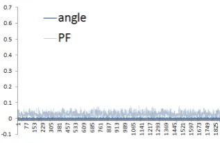
Control by sharing likelihood to estimate states: In Figure

10, the thick line indicates the actual observed value ofϕand the thin line indicates the estimated value of ϕ tracked by particle filter. From Figure 10, we see that the estimation of

ϕwith particle filter is almost correct. However, in the case that the amplitude of the inverted pendulum is extremely small, that is, almost 0, we see that the estimation is not so correct. Therefore, there is still space to consider improving the accuracy of the estimation with particle filter.

[image:4.595.343.505.468.560.2]

(5)

[image:5.595.341.512.49.232.2]

estimated by our proposed method.

Fig. 10. Angleϕ(with disturbances)

[image:5.595.87.247.79.179.2]

Fig. 11. Position of the inverted pendulum (with disturbances)

Fig. 12. Estimated forcefˆ(with disturbances)

VI. EXPERIMENT2: ROBUSTNESS FOR DISTURBANCES

To verify the robustness of our proposed control method, we conducted two additional experiments under different experimental settings. In the experiment 2, we use the same experimental settings in the experiment 1 except the settings of disturbances in the simulation environment. As Figure 13 and Figure 14 show, we have set the environment where there are more disturbances than those in the experiment 1. Furthermore, as well as the case expressed in Figure 13, in Figure 14 we increased the number of disturbances and enlarged each side of disturbances from 5.0(mm) to 10.0(mm).

A. Experimental results and discussions

The results of two additional experiments are shown from Figure 15 to Figure 20. Figures 15, 16, 17 show the result of

ϕandϕˆ,p, andfˆ, respectively, in the case where the number of disturbances increased as shown in Figure 13. The inverted pendulum could be controlled as it stood upright as well as the experiment 1 where there were 22 disturbances in the environment. Next, Figures 18, 19, 20 show the result of ϕ

andϕˆ,p, andfˆ, respectively, in the case where the number

[image:5.595.339.510.260.439.2]

Fig. 13. More disturbances whose side is5.0(mm)

Fig. 14. More disturbances whose side is10.0(mm)

and the size of disturbances are changed as shown in Figure 14. From those Figures, we see that at first the pendulum was widely swinging when hitting the disturbances but finally became stable and stood upright. Besides, we conducted another experiment with the settings for disturbances in which they exceed10.0(mm)on a side, but could not control as the pendulum stood up.

VII. CONCLUSIONS

[image:5.595.88.249.373.471.2]

(6)

[image:6.595.89.248.53.156.2] [image:6.595.343.509.56.155.2]

Fig. 15. Angleϕandϕˆ(More disturbances whose side is5.0(mm))

[image:6.595.89.249.194.304.2]

Fig. 16. Position of pendulum (More disturbances whose side is5.0(mm))

Fig. 17. Forcefˆto the cart (More disturbances whose side is5.0(mm))

In the experiment 1, we have confirmed that our method can estimate not directly observable states of a target by sharing the likelihood of the observable states of the target. By this, the control without the equation of motion can be achieved by our method.

In the experiment 2, we conducted an experiment of controlling an inverted pendulum in the environment where more disturbances exist rather than the environment in the experiment 1, and then have shown the robustness of our proposed method for controlling the pendulum.

As future work, we will explore the stability of control and improve the accuracy of estimation with particle filters.

[image:6.595.86.250.348.445.2]

Fig. 18. Angleϕandϕˆ(More disturbances whose side is10.0(mm))

Fig. 19. Position of pendulum (More disturbances whose side is 10.0(mm))

Fig. 20. Forcefˆto the cart (More disturbances whose side is10.0(mm))

REFERENCES

[1] T. Nishida, N. Ikoma, and S. Kurogi, Tracking and shape estimation

of deformable object using particle filter and adaptive vector quantizer,

No.190, WAC2010, 2010.

[2] L. Sun and S. Wang, Controlling inverted pendulum based on neural

network and particle filter, pp.1345 - 1348, Intelligent Control and

Automation, 2008.

[3] D. Stahl and J. Hauth, PF-MPC:Particle Filter-Model Predictive

Con-trol, System Control Letter, Vol.60, pp.632-643, 2011.

[4] H. Inoue, K. Hatase, and K. KAMEI, Fuzzy Classifier System Using

Hyper-Cone Membership Functions and Rule Reduction Techniques,

Proceedings of The 10th IEEE International Conference on Fuzzy Systems, pp.1436-1439, 2001.

[5] H. Inoue, K. Matsuo, K. Hatase, K. KAMEI, M. Tsukamoto and K. Miyasaka, A Fuzzy Classifier System Using Hyper-Cone Membership

Functions and Its Application to Inverted Pendulum Control,

Proceed-ings of 2002 IEEE International Conference on Systems, Man, and Cybernetics, Paper Number WA2D3(CD-ROM), 2002.

[6] K. Yamada, A. Yuzawa, and K. Nitta, Swing up control of inverted

pendulum using approximate linearization (in Japanese), Journal of

the Japan Society of Applied Electromagnetics and Mechanics, Vol.12, No.1, pp.62-72, 2004.

[7] Y. Kashimura, A. Ueno, and S. Tatsumi, A Continuous Action Space

Representation by Particle Filter for Reinforcement Learning (in Japanese), 2A1-3, The 22nd Annual Conference of the Japanese Society

for Artificial Intelligence, 2008.

[image:6.595.342.499.357.453.2]