Control of Yaw Angle and Sideslip Angle Based
on Kalman Filter Estimation for Autonomous EV
from GPS
Yongkang Zhou, Weijun Liu, Harutoshi Ogai
Abstract—The accurate measurements of yaw angle and sideslip angle are essential for autonomous EV dynamics control. A novel lateral stability control method using on-board GPS receiver is proposed. With proposed Kalman filter, GPS measurement delay is revised and yaw angle and sideslip angle could be estimated efficiently. On the other hand, we choose model predictive control(MPC) as an advanced control method to deal with the constrained optimal tracking problem in autonomous driving. At last, simulation and experiment results verify the effectiveness of proposed control system.
Index Terms—Autonomous driving, Lateral stability control, MPC
I. INTRODUCTION
R
APID development of autonomous driving EV tech-nology has improved the conservation and comfort of human’s transportation. However, few works focus on dynamic motion control. Actually, in the autonomous driving system, the accurate measurements of vehicle yaw angle and side slip angle at the center of gravity are essential for vehicle stability control (VSC). Therefore, we try to design the yaw angle and sideslip angle estimator by using single-antenna GPS receiver in order to reduce the cost and improve the safety of the autonomous driving system. Previously, yaw angle control and sideslip angle control are often realized by simple feedback controller like PD or PID[1]. In order to simplify and improve accuracy of the control system, model predictive control (MPC)[5] seems to be an effective method to control steering angle of the EV. Thus, we choose MPC as an advanced control method to deal with the constrained optimal tracking problem.II. VEHICLEMODELING
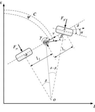
The planer 2-wheel model shown in Fig. 1 is used as the vehicle model. And parameters in the model are shown in TABLE I. Course angle is defined as the angle between direction of vehicle and geodetic North calculated by GPS data[4][7]. And sideslip angle is defined as the angle between velocity vector and longitudinal direction. Thus, we can obtain that course angle equals yaw angle plus sideslip
Manuscript received January 03, 2017; revised January 09, 2017. Yongkang Zhou with the master student at the School of Information, Production and System in Waseda university, Kitakyushu, Fukuoka province 8080135 Japan (email: [email protected]).
Weijun Liu with the master student at the School of Information, Production and System in Waseda university, Kitakyushu, Fukuoka province 8080135 Japan (email: [email protected]).
[image:1.595.341.507.200.396.2]Harutoshi Ogai is with the professor at the School of Information, Production and System in Waseda university, Kitakyushu, Fukuoka province 8080135 Japan (email: [email protected]).
Fig. 1: Planar 2-wheel model
angle with these definitions. Here, vehicle dynamics can be expressed by the following equations.
mv( ˙β+γ) =−2Cf(β+
lfγ
v −δ)−2Cr(β− lrγ
v ) (1)
I( ˙β+γ) =−2Cflf(β+
lfγ
v −δ) + 2Crlr(β− lrγ
v ) (2)
c=ψ+β (3)
And the state space model of vehicle’s yaw motion can be expressed as (4), (5) from (1), (2), and (3).
˙
x=Ax+Bu (4)
y=Cx+Du (5)
where,
x=
β γ ψ T , y=
ψ c T
, u=δ (6)
A=
a11 a12 0 a21 a22 0
0 1 0
, B=
b11 b21
0
(7)
C=
0 0 1
1 0 1
, D=
0 0
(8)
a11=−
2(Cf+Cr)
mv , a12=−1−
2(Cflf −Crlr)
mv2 (9)
a22=−
2(Cfl2f+Crlr2)
Iv , a21=−
2(Cflf−Crlr)
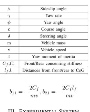
TABLE I: Parameters in model
β Sideslip angle
γ Yaw rate
ψ Yaw angle
c Course angle
δ Steering angle m Vehicle mass v Vehicle speed I Yaw moment of inertia
Cf,Cr Front/Rear concenring stiffness
lf,lr Distances from front/rear to CoG
b11=−
2Cf
mv , b21=−
2Cflf
mv (11)
III. EXPERIMENTALSYSTEM
[image:2.595.307.545.256.482.2]In this study, we select the PHEV “PRIUS” as the exper-imental vehicle which is developed by NEDO-PROJECT as shown in Fig. 2. It is applicable for autonomous driving using MicroAuto Box via dSpace. IMU is installed at the center of gravity (CoG) to measure the yaw angle. A single-antenna GPS receiver, the Hemisphere A325, is used to provide vehicle position to calculate course angle with the update rate of 10Hz. The accuracy of longitude and latitude near to 1 centimeter level under real-time kinematic mode(RTK). Datas of these sensors are transferred by ROS. ROS is connected with MicroAuto Box by LAN.
Fig. 2: Experimental vehicle and GPS receiver.
IV. CONTROLSYSTEMDESIGN
A. Estimation Design
In this section, the idea of multi-rate output measurements is applied for robust estimation of sideslip angle and yaw angle. The state space (4), (5) is transformed to the discrete form[2]:
xk+1=Gk·xk+Hk·uk+wk (12)
yk =Ck·xk+vk (13)
where wk is process noise and vk is measurement noise.
wk and vk are assumed to be constructed by Gaussian
distribution with zero mean. And, here
Gk=eA·Tc, Hk = Tc
Z
0
eA·τ·Bdτ, Ck =C (14)
Use the previous one-step information to define discretized system, then we can obtain:
xak+1=G
a k·x
a k+H
a
k ·uk+wk (15)
yka=Cka·xak+vk (16)
where,
Gak =
Gk TcI
0 I
, Hka =
Hk
0
. (17)
1) Multi-rate Measurements: In this Kalman filter design[3], yaw angle and course angle are selected as output measurements. While yaw angle’s sampling time from IMU can be same as control period atTc(1ms), the sampling time
of course angle from GPS receiver is much longer atTs(100
ms). To solve this multi-rate problem, we proposed to set pseudo-samples between two consecutive updates of course angle as shown in Fig. 3. During pseudo-samples, there is no course angle update. Therefore, we can build measurement matrixCa
k in two cases as in (18)(19).
If course angle is updated:
Cka=
0 0 1 0 0
1 0 1 0 0
; (18)
and during pseudo-samples:
Cka=
0 0 1 0 0
0 0 0 0 0
. (19)
Fig. 3: Two sampling times of output measurements.
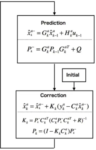
2) Kalman Filter Algorithm: There are two parts, time update part and measurement update part in Kalman filter recursive algorithm. They are built by the following equa-tions.
Time update:
ˆ
xak−=Gakxˆka−1+Hkauk−1 (20)
Measurement update:
ˆ
xak= ˆxak−+Kk(yak−C a kxˆ
a−
k ) (21)
Error covariance is constructed as follows:
Pk−=GakPk−1GaTk +Q (22)
then update the error covariance:
Pk= (I−KkCka)Pk− (23)
To calculate the Kalman Gain, we use the function:
Kk=Pk−C aT k (C
a kPk−C
aT k +R)−
1
(24)
Here, process noise covariance is
Q=E wk wkT
[image:2.595.56.284.410.493.2]
Fig. 4: Kalman filter alogrithm.
and measurement noise covariance is
R=E
vk vkT
. (26)
From the descriptions above, the block diagram of Kalman filter algorithm can be constructed in the Fig. 4. Q and R are the process noise and measurement noise covariance matrices. They are tuning parameters of the Kalman filter. If R is too large, the Kalman gain decreases, thus, the estimation fails to update the subsequent disturbances based on measurements. GPS impacts on the variances of yaw angle noise and course angle noise respectively. And these noises are chosen based on measurement of course angle from GPS because of its validity. On the other hand, large Q leads the estimation to rely on the measurements.
B. Controller Design
The block diagram of the whole control system is shown in Fig. 5. In the following sub-sections, we will explain the design of this proposed system.
1) Reference Model: In this study, we choose the simplest way in autonomous navigation: point-to-point[8]. To calcu-late the command of desired steering angle to navigate the vehicle from point (x1,y1) to point (x2,y2) with following
equations.
δ=
tan−1
x2−x1 y2−y1
, y2> y1
π−tan−1 x
2−x1 y2−y1
, y2< y1, x2> x1
tan−1 x
2−x1 y2−y1
−π, y2< y1, x2< x1
(27)
A long path can be divided into several segments. In each segment, steering angle reference is kept constant.
And the reference model is designed based on the steady-state response of sideslip angle and yaw angle by using the model in Section II. The following equations express the calculation of reference values from the command of steering angle.
ψ(s) =G(s)δ(s) =
− b21s+ (a21b11−a11b21)
s3+ (−a
11−a22)s2+ (a11a22−a12a21)s
δ(s) (28)
β(s) =G(s)δ(s) =
− b11s+ (a12b21−a22b11)
s2+ (−a
11−a22)s+ (a11a22−a12a21)
δ(s) (29)
2) MPC Controller: As we can see, the problem in
autonomous driving system is that it is hard for tracking command of the steering angle. Therefore, it is natural for us to think about model predictive control (MPC)[5][6]. Firstly, MPC is a model based control method. It uses dynamic model explicitly, to predict the future behavior of the system. Secondly, MPC is an optimal control method, it has a quadratic cost function. The control law is obtained by minimizing the cost function. By adjusting the weights, the trade-offs could be shifted. Thirdly, MPC could consider the input constraints in solving the optimal problem. MPC could consider all the problems above. The concept of MPC is simple. A quadratic cost function of future behavior is established and by finding a series of optimal input, the cost function is minimized. The first one of the optimal input is implemented and the procedures are repeated again in the next step.[5]
In the procedures, there are three parts: prediction part, optimization part, and implementation part.
In the prediction part,
xk+1=Axk+Buk (30)
x1=Ax0+Bu0 (31)
x2=Ax1+Bu1 (32)
. . . (33)
xN =AxN−1+BuN−1 (34)
inputs u0,u1,. . .,uN−1 and current statex0 are unknown
parameters.
And when we come to optimization part,
min
z }| {
(u0, u1, . . . , uN−1)J (35)
J is the cost function,
J=X
k
xTkQdxk+uTkRuk+ ∆uTkR∆uk) (36)
then, we could calculate the first optimal input u0 in the
Fig. 5: Overview of proposed control system.
a)
c)
b)
d)
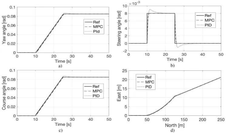
Fig. 6: Cornering test(simulation result).
a) Yaw angle; b) Course angle; c) Steering angle; d) Trajectory of vehicle.
V. CONTROLSYSTEMVERIFICATION
A. Control-Simulation Results
In autonomous driving system, we need verify two aspects of vehicle’s performance: straight driving and cornering. In the simulation, vehicle velocity is kept at 25 km/h in constant, and the general system with feed forward and feedback controllers (PID) are performed for comparison. To verify the robust issue, simulation results are summarized as follows in two cases: In cornering simulation, Fig. 6 (a)(b) illustrates the responses of vehicle yaw angle and course angle according to different control schemes; (b) expresses the front steering angles which are the control inputs; (d) performs the trajectories of vehicle motion. Also, we made lane changing test shown as Fig. 7 to make sure the control system perform well in real autonomous driving process.
B. Control-Experimental Results
To evaluate the proposed control scheme, we conduct the autonomous driving test. In the experiment, the vehicle
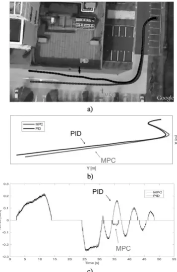
trajectory is desired to be driving to exit from parking lot automatically. Steering angle reference is pre-calculated by using formulation (27). The trajectory results are displayed in Google Earth and Plot XY as shown in Fig. 8. As a result, the tracking of yaw angle, course angle and trajectory are successfully achieved. Thus, we can clearly see that when applying the proposed control scheme, tracking performance is very well.
VI. CONCLUSION
[image:4.595.108.481.273.493.2]a)
c)
b)
[image:5.595.110.479.58.279.2]d)
Fig. 7: Lane changing test(simulation result).
a) Yaw angle; b) Course angle; c) Steering angle; d) Trajectory of vehicle.
Fig. 8: Autonomous driving test. a) Experimental trajectory (in GRS 80); b) Experimental trajectory (in XY plot);
c) Yawrate (observed by IMU).
In this paper, sensors fusing is still too simple. We have to consider environmental factors as disturbance. In future work, we will accomplish more autonomous driving tests with supplementary systems of laser sensors[9] and cameras to improve automatic driving performance.
REFERENCES
[1] Masao Nagai, P. RAKSINCHAROENSAKCar robotics, 2rd ed. ZMP publishing, 2010.
[2] Molinder S. Grewal, Angus P. AndrewsKalman Filtering - Theory and Practice Using MATLAB, 3rd ed. Wiley-IEEE Press, 2008. [3] Nguyen, Binh Minh, et al. ”Dual rate Kalman filter considering delayed
measurement and its application in visual servo.” 2014 IEEE 13th International Workshop on Advanced Motion Control (AMC).IEEE, 2014.
[4] Ryu, Jihan, Eric J. Rossetter, and J. Christian Gerdes. ”Vehicle sideslip and roll parameter estimation using GPS.”Proceedings of the AVEC International Symposium on Advanced Vehicle Control. 2002.
[5] J.M. Maciejowski ,Predictive Control with Constraints, 1st ed. Pren-tice Hall, 2000.
[6] Magni Lalo; Scattolini, Riccardo. Robustness and robust design of MPC for nonlinear discrete-time systems. In:Assessment and future directions of nonlinear model predictive control. Springer Berlin Heidelberg, 2007. p. 239-254.
[7] Bevly, David M., Jihan Ryu, and J. Christian Gerdes. ”Integrating INS sensors with GPS measurements for continuous estimation of vehicle sideslip, roll, and tire cornering stiffness.”IEEE Transactions on Intelligent Transportation Systems7.4 2006: 483-493.
[8] Choi, Ji-wung; Curry, Renwick; Elkaim, Gabriel. Path planning based on bzier curve for autonomous ground vehicles. In:World Congress on Engineering and Computer Science 2008, WCECS’08. Advances in Electrical and Electronics Engineering-IAENG Special Edition of the. IEEE, 2008. p. 158-166.
[9] Guivant Jose; Nebot, Eduardo; Baiker, Stephan. Autonomous navigation and map building using laser range sensors in outdoor applications.
[image:5.595.78.257.348.623.2]