SPATIO-TEMPORAL MODELLING DAM
DEFORMATION USING INDEPENDENT COMPONENT ANALYSIS
Wujiao Dai1, Bin Liu1, Xiaolin Meng2, Dawei Huang1
1) Dept. of Surveying Engineering & Geo-informatics, Central South University, Changsha, China
2) Nottingham Geospatial Institute, the University of Nottingham, UK [email protected](*corresponding author)
ABSTRACT
Modelling dam deformation based on the monitoring data plays an important role in the assessment of a dam’s safety. Traditional dam deformation modelling methods generally utilize single monitoring points. It means it is necessary to model for each monitoring point and the spatial correlation between
points will not be considered using traditional modelling methods. Spatio-temporal modelling methods
provide a way to model the dam deformation with only one functional expression and analyze the
stability of dam in its entirety. Independent Component Analysis (ICA) is a statistical method of Blind
Source Separation (BSS) and can separate original signals from mixed observables. In this paper, ICA
is introduced as a spatio-temporal modelling method for dam deformation. In this method, the
deformation data series of all points were processed using ICA as input signals, and a few output
independent signals are used to model. The real data experiment with displacement measurements by
wire alignment of Wuqiangxi Dam was conducted and the results show that the output independent
signals are correlated with physical responses of causative factors such as temperature and water level
respectively. This discovery is beneficial in analyzing the dam deformation. In addition, ICA is also an
effective dimension-reduced method for spatio-temporal modelling in dam deformation analysis
applications.
Keywords: Dam Deformation Analysis; Independent Component Analysis; Spatio-temporal modeling
INTRODUCTION
Two main methods, statistical analysis and structural identification, are usually used in the area of dam deformation monitoring. From the result of comparison between statistical analysis and structural identification (De Sortis and Paoliani, 2007), the statistical model has the advantages of simplicity for functional expression, fast execution and suitability to any kind of correlation between the governing and dependent parameters. But the statistical parameters do not have any physical meaning, which is not conducive to interpreting the dam deformation. The method of blind source separation (BSS) was used to separate contributions of external loads to the displacements from the deformation data of several points on the dam (Popescu, 2011). Popescu’s work showed that the “all points, one model” (i.e. spatio-temporal model) with physical meaning parameters is possible for dam statistical deformation modelling. Independent component analysis (ICA) is a method of blind source separation proposed in 1990s, which transforms the observed mixed signals into a series of signals whose components are mutually independent in statistical sense. Since independent component indicates some physical meaning in some case, ICA can be taken as a data mining tool. In this paper, we applied ICA to extract the independent displacement components from the monitoring data of 11 points measured by wire alignment on Wuqiangxi Dam and analyzed the correlation between the independent displacement components and causative factors such as temperature and water level. Then, a spatio-temporal displacement model of Wuqiangxi Dam was established using the extracted independent components and the corresponding spatial response values to the monitoring points.
In this paper, the fundamental theory of ICA and the FastICA algorithm are introduced in Section 2. The deformation monitoring data and the independent displacement components of Wuqiangxi Dam are analyzed in Section 3. The steps of spatio-temporal modelling using ICA are described in detail in Section 4. The spatio-temporal displacement model of Wuqiangxi dam deformation is established and the result analysis is described in Section 5. Finally, the conclusions are presented in Section 6.
INDEPENDENT COMPONENT ANALYSIS (ICA)
Basic model of ICA
ICA is a useful method for blind source separation. Its fundamental principle can be
illustrated using Figure 1. Suppose that there are M observations X ,
T M(t)
, (t),
(t) [X1 X ]
X , from N independent components Si(t),i 1,2,,N, we
have:
N M (t) (t)AS ;
X (1)
Without any other priori information about matrix A or source signals, ICA aims
to obtain a separating matrix W to separate the original signals S(t) in Eq. 1 based
on some optimization criteria and learning methods. Generally, the process of
calculating W can be divided into two steps: 1) Whiten the observed signals X(t) by
a whitening matrix B, to let Z BX and E(ZZT)I (Iis a unit matrix). 2)
Calculate the rotation matrix by the specific independence optimize rule, to let
UZ
Y(t) , where Y(t) is the best approximation vector of S(t). FastICA Algorithms
ICA algorithms can be divided into two main categories, and both of them are based on the non-gaussianity and independence of the source signals. The FastICA is a fast optimization iterative algorithm with a good stability (Hyvärinen, 1999; Hyvärinen and Oja, 2000). It is based on the negentropy which is a common quantitative measure of the non-gaussianity of a random variable. The stronger the non-gaussianity of a random variable is, the greater the negentropy will be. The detailed steps are as follows:
1. Centralize and whiten the observed data.
2. Choose an initial weight vector of unit norm (random) w.
3. Update w through w(k1)E[xg(wT(k)x)]E[g'(wT(k)x)]w.
4. Normalizate w by
) 1 (
) 1 ( ) 1 (
k k k
w w
w .
5. Go back to step (3) if not converged..
INDEPENDENT DISPLACEMENT COMPONENTS OF WUQIANGXI DAM
Wuqiangxi Dam and Its Monitoring Data
Fig. 2. Picture of Wuqiangxi Dam
Two tension wire alignments are mainly used to monitor the horizontal displacements of the Wuqiangxi Dam. The displacement data of 12 different monitoring points in the second tension wire alignment was selected for the spatio-temperal modelling experiment, in which 11 points are used to model and another point is used to check the accuracy of the model. The measurements of water level (the difference between the water level of upstream and downstream) and air temperature are also collected for the modelling experiment. All the data are measured daily. The displacement data series of the 11 points are shown in Fig. 3 and the data series of causative factors, including air temperatures and water level, are shown in Fig. 4.
2005 2009
-10 0 10
ex
2-11
(m
m
)
2005 2009
-10 0 10
ex
2-12
(m
m
)
2005 2009
-10 0 10
ex
2-13
(m
m
)
2005 2009
-10 0 10
ex
2-14
(m
m
)
2005 2009
-10 0 10
ex
2-15
(m
m
)
2005 2009
-10 0 10
ex
2-17
(m
m
)
2005 2009
0 10 20
ex
2-18
(m
m
)
2005 2009
0 10 20
ex
2-19
(m
m
)
20050 2009
10 20
ex
2-20
(m
m
)
Date(year)
20050 2009
10 20
ex
2-21
(m
m
)
Date(year)
20050 2009
10 20
ex
2-22
(m
m
)
[image:4.595.95.465.246.412.2]Date(year)
Fig. 3. Displacement data series of the 11 monitoring points
2005 2006 2007 2008 2009 2010 -10
0 10 20 30 40
Te
m
pe
ra
tu
re
(
℃
)
Date(year)
2005 2006 2007 2008 2009 2010 35
40 45 50 55 60
W
at
er
le
ve
l(m
)
[image:4.595.81.484.459.589.2]Date(year)
Fig. 4. Data series of water level and air temperature
Common Displacement Components Separation
2005 2006 2007 2008 2009 2010 -2
0 2
IC
1(
m
m
)
2005 2006 2007 2008 2009 2010
-3 0 3
IC
2(
m
m
)
2005 2006 2007 2008 2009 2010
-5 0 5
IC
3(
m
m
)
[image:5.595.167.352.66.204.2]Date(year)
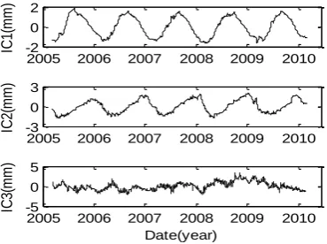
Fig. 5. Independent components extracted from the data of dam displacements
To probe the relationship between ICs and causative factors, comparisons are made between some ICs and air temperature and water level as shown in Fig. 6. All the data
have been standardized with mean 0 and variance 1 by
S X X
Z (X is the mean
value and S is the variance) and adjusted in the same sign in order to make clear comparisons. It can be noted that, the common components of each point extracted by ICA have strong correlation with the air temperature and water level. The data series of IC1 has the similar variation with the data series of air temperature, and a lag effect exists at the same time, which is consistent with the effect of air temperature to the dam deformation (He, 2010). The data series of IC2 has a similar variation with the data series of water level, which means IC2 represents the common water level displacement response of each point. IC3 has no obvious features and it has a little spatial response to each point of the dam. We guess it may be due to the other unknown external loads or some minor combined effects of water level and air temperature on the dam deformation.
From the above results and analysis, it can be concluded that ICA can extract the independent displacement components which can be correlated with the causative factors respectively without a priori knowledge.
2005 2006 2007 2008 2009 2010 -4
-2 0 2 4
Date(year)
IC
1
an
d
Te
m
pe
ra
tu
re
2005 2006 2007 2008 2009 2010 -4
-2 0 2 4
Date(year)
IC
2
an
d
W
at
er
L
ev
el
temperature
IC1
w ater level
IC2
(b) (a)
Fig. 6. Comparison between ICs and environmental factorsSpatio-temporal Model based on ICA
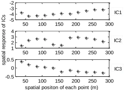
[image:5.595.88.473.553.683.2]displacements over an entire structure (i.e. spatio-temporal model) and to describe its global behavior with only a few independent components. Furthermore, each independent component is related to only one causative factor. When extracting the independent displacement components using ICA, we can also get the spatial response values of ICs for each point to the dam displacements from the mixing matrix. The spatial response values of ICs to each point are shown in Fig.7, from which it seems that the response values may be related to the structure of the dam.
50 100 150 200 250 300 -5
-4 -3 -2
50 100 150 200 250 300 1
2 3 4
s
p
a
ti
a
l
re
s
p
o
n
s
e
o
f
IC
s
50 100 150 200 250 300 -0.5
0 0.5
spatial positon of each point (m)
IC1
IC2
[image:6.595.158.376.184.341.2]IC3
Fig. 7. Spatial response values of ICs to each point
From the displacement measurements of each point, we can see that the displacement responses to the external loads are different. From the physical view, it is due to different structure features and external loads in the different positions. However, as an entire structure, there will be an entire displacement response to external loads. This entire displacement can be measured by all monitoring points although it hides in the displacement data of the points. The three independent displacement components extracted from data of the 11 points using ICA can be interpreted as the entire displacement responses to hydrostatic load, thermal effect and time effect or other unknown external loads. The spatial response values of ICs reflect the different displacement responses to external loads in different positions. From the fundamental principle of ICA, the displacement of a point is the entire displacement response multiplying the corresponding spatial response value. It means that the spatio-temporal modelling procedures can be divided to spatial modelling with spatial response values and temporal modelling with displacement ICs respectively.
The steps of spatio-temporal modelling dam deformation based on ICA are shown as follows:
1. Extract the independent components (ICs) from the observed monitoring data X using FastICA algorithms and the ICs and the mixing matrix Acan be obtained. Then
3 , 2 , 1 ,
A ICs s
X .
2. Model each independent component with suitable methods (dam statistical modelling such as HHT and HTS or geometrical modelling such as curve fitting).
the points are on one line of wire alignment, the spatial response models of the ICs are
curve functions Rs(x), where s1,2,3 and x is the positions of the points.
4. Space fit the constant displacements using a surface function (in two dimension
case) or a curvilinearfunction (in one dimension case) Dcons(x).
5. Multiply the temporal models of ICs and the spatial response functions Rs(x)and
add the spatial constant displacement function Dcons(x)to get the spatial-temporal displacement model of the dam D(x) ICsRs(x)Dconst(x), where s1,2,3 and x
is the positions of the points.
As indicate above in step 2), the three displacement component need to be modeled using statistical modelling or geometrical modelling methods. According to the analysis before, IC1 is related to air temperature and IC2 is related to water level. So we establish the models of IC1 and IC2 using the temperature and water level components in the dam HHT model respectively. The function model of IC1 is Equ. 2.
i i
i a
a T
IC
4
1 0
1 (2)
where Ti means the average temperature of 0-1, 2-7, 8-30 and 31-60 days before
because of the lag effect between the temperature of dam and the environment. The function model of IC2 is Equ. 3.
4
1 0 2
i i i b
b H
IC (3)
where H denote the difference of water level between upstream and downstream. Since the physical meaning of IC3 is not clear, we a curve fitting method with equation (4) to model IC3.
) sin(
) sin(
) sin(
) sin(
4 4 4
3 3 3 2 2 2 1 1 1 3
c t b a
c t b a c t b a c t b a
IC
(4)
SPATIO-TEMPORAL MODEL OF WUQIANGXI DAM AND ITS STATISTICAL ANALYSIS
2005 2007 2009 -2 0 2 Date(year) D is p la c e m e n t( m m )
2005 2007 2009
-2 0 2 4 Date(year) D is p la c e m e n t( m m )
2005 2007 2009
-4 -2 0 2 4 Date(year) D is p la c e m e n t( m m ) IC1 fitting value IC2 fitting value IC3 fitting value
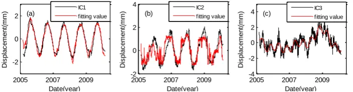
[image:8.595.91.443.67.159.2](a) (b) (c)
Fig. 8. The fitting results of external load of air temperature (a), water level (b) and other factors(c) after modelling the ICs.
Spatial response values of each displacement component are obtained from the mixing matrix, with which the three spatial response function models are established using curvilinearfitting method. Equ. (5), (6) and (7) are the spatial response functions of IC1, IC2 and IC3 respectively. The fitting results are shown in Fig. 9.
i i ix p p (x) R
5 1 01 (5)
2 3 3 2 2 2 2 1 1 3 2 1 2 ) c b x ( ) c b x ( ) c b x ( e a e a e a (x) R (6)
2 1 0 3 i i ix p p (x)R (7)
The constant displacements in the 11 points are fitted using a curvilinearfunction as Equ. (8) and the fitting results are shown in Fig. 10.
w)) x (i b w) x (i (a a (x) i i i
const
sin cos 3 1 0 D (8)
50 100 150 200 250 300 -6
-4 -2
50 100 150 200 250 300 0 2 4 s p a ti a l re s p o n s e f u n c ti o n o f IC s
50 100 150 200 250 300 -0.5
0 0.5
spatial position (m)
IC2 IC1
[image:8.595.173.466.287.397.2]IC3
50 100 150 200 250 300 -5
0 5 10 15
spatial positions (m)
c
o
n
s
ta
n
t
d
is
p
la
c
e
m
e
n
ts
(m
m
)
[image:9.595.155.368.60.193.2]obseved values fitting values
Fig. 10. The fitting results of the constant displacements
At last, the dam displacement spatio-temporal model is established as Equ. (9).
(x) (x)
R
(x) R (x)
R (x)
const D IC
IC IC
D
3 3
2 2 1
1
(9)
where x is the position in the tension wire alignment line.
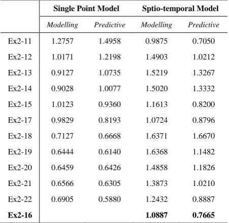
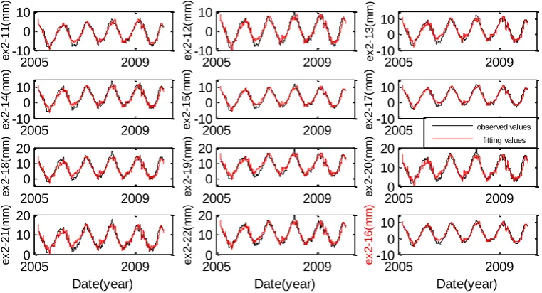
As we known, one of the main purposes of modelling the dam displacement is to predict the displacement of dam. In order to verify the effectiveness of spatio-temporal model shown as Equ. (9), the predicted displacements of 100 days for all points using spatio-temporal model and traditional single point models are compared. The results shown in table 1 indicate that both models can predict displacement with a high accuracy, but the prediction accuracy of single point model is higher than the one of spatio-temporal model. However, from the predicted displacement of point ex2-16 whose data hasn’t been used to establish the model, spatio-temporal model still can predict the displacement with a high accuracy. Obviously, compared to the single point model the advantage of the spatio-temporal model can predict the displacement of any position of the dam no matter where there is a monitoring point. The results of fitting and prediction of the spatio-temporal model are shown in Fig. 11 and Fig. 12.
Table 1. The RMS values of predicted displacement error and modelling error of each point using different models
Single Point Model Sptio-temporal Model
Modelling Predictive Modelling Predictive
Ex2-11 1.2757 1.4958 0.9875 0.7050
Ex2-12 1.0171 1.2198 1.4903 1.0212
Ex2-13 0.9127 1.0735 1.5219 1.3267
Ex2-14 0.9028 1.0077 1.5020 1.3332
Ex2-15 1.0123 0.9360 1.1613 0.8200
Ex2-17 0.9829 0.8193 1.0724 0.8796
Ex2-18 0.7127 0.6668 1.6371 1.6670
Ex2-19 0.6444 0.6140 1.6368 1.1482
Ex2-20 0.6459 0.6426 1.4858 1.1826
Ex2-21 0.6566 0.6305 1.3873 1.0210
Ex2-22 0.6905 0.5880 1.2432 0.8887
[image:9.595.154.380.548.768.2]2005 2009 -10 0 10 e x 2 -1 1 (m m ) 2005 2009 -10 0 10 e x 2 -1 2 (m m ) 2005 2009 -10 0 10 e x 2 -1 3 (m m ) 2005 2009 -10 0 10 e x 2 -1 4 (m m ) 2005 2009 -10 0 10 e x 2 -1 5 (m m ) 2005 2009 -10 0 10 e x 2 -1 7 (m m ) 2005 2009 0 10 20 e x 2 -1 8 (m m ) 2005 2009 0 10 20 e x 2 -1 9 (m m )
20050 2009 10 20 e x 2 -2 0 (m m )
20050 2009 10 20 Date(year) e x 2 -2 1 (m m ) 2005 2009 -10 0 10 Date(year) e x 2 -1 6 (m m )
[image:10.595.92.473.70.276.2]20050 2009 10 20 Date(year) e x 2 -2 2 (m m ) observed values fitting values
Fig. 11. Fitting results of the 11points and an checking point (ex2-16) using the spatio-temporal
model 2010/03/01 2010/06/01 -5 0 5 e x 2 -1 1 (m m ) 2010/03/01 2010/06/01 -10 0 10 e x 2 -1 2 (m m ) 2010/03/01 2010/06/01 0 5 10 e x 2 -1 3 (m m ) 2010/03/01 2010/06/01 0 5 10 e x 2 -1 4 (m m ) 2010/03/01 2011/06/01 0 5 10 e x 2 -1 5 (m m ) 2010/03/01 2011/06/01 0 5 10 e x 2 -1 7 (m m ) 2010/03/01 2010/06/01 0 10 20 e x 2 -1 8 (m m ) 2010/03/01 2010/06/01 5 10 15 e x 2 -1 9 (m m ) 2010/03/01 2010/06/01 5 10 15 e x 2 -2 0 (m m ) 2010/03/01 2010/06/01 5 10 15 Date e x 2 -2 1 (m m ) 2010/03/01 2010/06/01 5 10 15 20 Date e x 2 -2 2 (m m ) 2010/03/01 2010/06/01 0 5 10 Date e x 2 -1 6 (m m ) observed values predicted values
Fig. 12. Predicted results of the 11points and an checking point (ex2-16) using the spatio-temporal
model
CONCLUSION
1. ICA can effectively extract the common displacement components caused by different external loads such as water level and temperature. This is beneficial to the physical interpretation of dam deformation.
2. Spatial correlation between the points can be reflected by the spatial response values of ICs.
[image:10.595.98.496.348.569.2]respectively. So, ICA can be used as an effective spatio-temporal modelling tool.
4. The spatio-temporal model using ICA provides a way to model the dam deformation with only one functional expression and analyze the stability of dam in its entirety.
5. Spatio-temporal model can predict the displacement of any position of the dam no matter where there is a monitoring point.
ACKNOWLEDGMENT
This work was supported by the National Natural Science Foundation of China (Grant No. 41074004) and the State Key Development Program of Basic Research of China (Grant No. 2013CB733303). The authors would like to thank Dr. Oluropo Ogundipe for polishing the writing.
References
1. Ardito, R., Maier, G., and Massalongo, G., 2008. Diagnostic analysis of concrete dams based on seasonal hydrostatic loading. Engineering Structures, 30 (11), pp. 3176-3185.
2. He J. P., 2010. Dam Safety Monitoring Theory and Its Application, China Water Power Press. 263 pages. (In Chinese)
3. Hyvärinen, A., 1999. Fast and robust fixed-point algorithms for independent component analysis. IEEE Trans on Neural Networks, 10 (3), pp. 626-634.
4. Hyvärinen, A., and Oja, E., 2000. Independent component analysis: algorithms and applications. Neural Networks, 13 (4-5), pp. 411-430.
5. Mata, J., 2011. Interpretation of concrete dam behaviour with artificial neural network and multiple linear regression models. Engineering Structures, 33 (3), pp. 903-910.
6. Popescu, T. D., 2011. A new approach for dam monitoring and surveillance using blind source separation. International Journal of Innovative Computing, Information and Control, 7 (6), pp. 3811-3824.
7. Sortis, A. De., and Paoliani, P., 2007. Statistical analysis and structural identification in concrete dam monitoring. Engineering Structures, 29 (1), pp. 110-120.
8. Szostak-Chrzanowski, A., Chrzanowski, A., and Massiéra, M., 2005. Use of deformation monitoring results in solving geomechanical problems—case studies. Engineering geology, 79 (1-2), pp. 3-12.
9. Xi, G. Y., Yue, J. P., Zhou, B. X., and Tang, P., 2011. Application of an artificial immune algorithm on a statistical model of dam displacement. Computers and Mathematics with Applications, 62 (10), pp. 3980-3986.