http://wrap.warwick.ac.uk/
Original citation:
LHCb Collaboration (Including: Back, J. J., Dossett, D., Gershon, T. J., Harrison, P. F.,
Latham, Thomas, Pilar, T., Poluektov, Anton, Reid, M. M., Whitehead, M. and Williams,
M. P.). (2012) Measurement of the B s 0-B - s 0 oscillation frequency δm s in B s 0→D s
-(3)π decays. Physics Letters B, Volume 709 (Number 3). pp. 177-184.
Permanent WRAP url:
http://wrap.warwick.ac.uk/44735
Copyright and reuse:
The Warwick Research Archive Portal (WRAP) makes this work of researchers of the
University of Warwick available open access under the following conditions.
This article is made available under the Creative Commons Attribution- 3.0 Unported
(CC BY 3.0) license and may be reused according to the conditions of the license. For
more details see
http://creativecommons.org/licenses/by/3.0/
A note on versions:
The version presented in WRAP is the published version, or, version of record, and may
be cited as it appears here.
Physics Letters B 709 (2012) 177–184
Contents lists available atSciVerse ScienceDirect
Physics Letters B
www.elsevier.com/locate/physletb
Measurement of the
B
0
s
–
B
0
s
oscillation frequency
m
s
in
B
0
s
→
D
−
s
(
3
)
π
decays
✩
.
LHCb Collaboration
a r t i c l e
i n f o
a b s t r a c t
Article history:
Received 21 December 2011
Received in revised form 3 February 2012 Accepted 10 February 2012
Available online 15 February 2012 Editor: W.-D. Schlatter
The B0
s–B0s oscillation frequencyms is measured with 36 pb−1 of data collected in pp collisions at √s
=7 TeV by the LHCb experiment at the Large Hadron Collider. A total of 1381 B0
s→D−s
π
+ and B0s →D−s
π
+π
−π
+ signal decays are reconstructed, with average decay time resolutions of 44 fs and 36 fs, respectively. An oscillation signal with a statistical significance of 4.6σ
is observed. The measured oscillation frequency isms=17.63±0.11(stat)±0.02(syst)ps−1.©2012 CERN. Published by Elsevier B.V. All rights reserved.
1. Introduction
After the observation ofB0–B0 mixing and the measurement of
its strength in 1987[1], it took a further 19 years for the B0
s–B0s
frequency to be measured for the first time [2,3]. This is mainly due to the fact that the B0
s–B0s oscillation frequency is 35 times
larger than that for theB0–B0system, posing a considerable
chal-lenge for the decay time resolution of detectors. For the LHCb experiment, the ability to resolve these fastB0
s–B0s oscillations is a
prerequisite for many physics analyses. In particular it is essential for the study of the time-dependentCPasymmetry ofB0s
→
J/ψφ
decays[4]. The oscillation frequency in theB0s–B0s system is given
by the mass difference between the heavy and light mass eigen-states,
ms (we use units with h
¯
=
1). In this Letter, we report ameasurement of
msby the LHCb experiment with data collected
in 2010.
The LHCb spectrometer covers the pseudo-rapidity range 2 to 5. In this region,b hadrons are produced with a large Lorentz boost and have an average flight path of 7 mm. The LHCb detector con-sists of several components arranged along the LHC beam line. The vertex detector (VELO) surrounds the collision point, followed by a first Ring Imaging Cherenkov (RICH) counter, a tracking station, a dipole magnet, three more tracking stations, a second RICH de-tector, a calorimeter system and a muon detector. The calorimeter system consists of a scintillating pad detector (SPD), a preshower detector, an electromagnetic calorimeter and a hadronic calorime-ter. A detailed description of the detector can be found in Ref.[5]. The precise spatial resolution of the VELO results in an impact pa-rameter resolution of 20–50 μm in the x and y directions1 for charged particles with transverse momenta in the range relevant for B0s daughter tracks used in this analysis. The x and y
resolu-✩ © CERN for the benefit of the LHCb Collaboration.
1 LHCb uses a right-handed Cartesian coordinate system with thex direction
pointing inside the LHC ring, theydirection pointing upwards and thezdirection running along the beamline from the interaction point towards the spectrometer.
tion in the position of the primary vertex reconstruction is about 15 μm while the z resolution is about 80 μm. This excellent per-formance results in the decay time resolution needed to observe the fastB0s–B0s oscillations. The invariant mass resolution provided by the tracking system and the
π
/
K separation given by the two RICH detectors provide clean B0s meson signals with small
back-ground. The particle identification capabilities of the RICH together with the calorimeter and muon systems allow the initial flavour of the B0
s to be tagged using charged kaons, electrons and muons,
respectively.
In the next section, the data sample used and the analysis strat-egy are introduced. This is followed by descriptions of the analysis of the invariant mass and decay time distributions, and the flavour tagging. Finally, we discuss the fit result for the oscillation fre-quency and the associated systematic uncertainties.
2. Data sample and analysis strategy
The analysis uses B0s candidates reconstructed in four
flavour-specific decay modes,2 namely B0
s
→
D−s(φ (
K+K−)
π
−)
π
+, B0s→
D−s
(
K∗0(
K+π
−)
K−)
π
+, B0s→
D−s(
K+K−π
−)
π
+ and B0s→
D−s(
K+K−π
−)
π
+π
−π
+. To avoid double counting, candidates that pass the selection criteria of one mode are not considered for the following modes. All reconstructed decays are flavour-specific final states, thus the flavour of the B0s at the time of its decay is given by the charges of the final state particles of the decay. A combination of tagging algorithms is used to identify the B0s
flavour at production. The algorithms provide for each event a tag-ging decision as well as an estimate of the probability that this decision is wrong (mistag probability). These algorithms have been optimized and calibrated using large event samples of flavour-specific B
→
μ
+D∗−X and B+→
J/ψ
K+ decays and a sample ofB0→
D−π
+decays.2 Unless explicitly stated, inclusion of charge-conjugated modes is implied.
0370-2693/©2012 CERN. Published by Elsevier B.V. All rights reserved.
178 LHCb Collaboration / Physics Letters B 709 (2012) 177–184
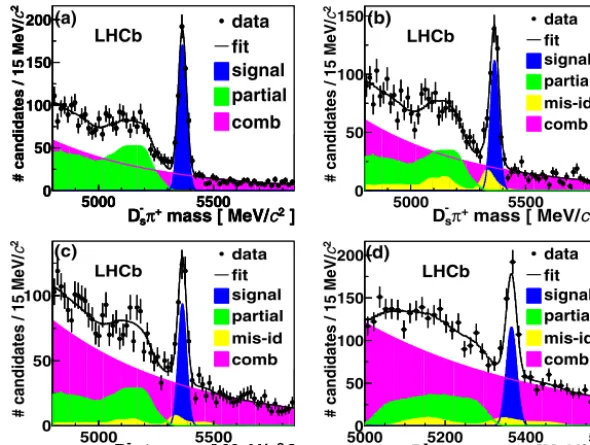
Fig. 1.Mass distributions for (a)B0
s→D−s(φπ−)π+, (b)B0s→D−s(K∗0K−)π+, (c)B0s→D−s(K+K−π−)π+and (d)B0s→D−sπ+π−π+candidates. The fits and the various
background components are described in the text. “Partial” refers to background from partially reconstructedB0
s decays, “mis-id” refers to background from fully or partially
reconstructedB0and
Λbdecays with one mis-identified daughter particle, and “comb” refers to combinatorial background.
The analysis is based on a data set of 36 pb−1 of pp
colli-sions at
√
s=
7 TeV collected in 2010. The first trigger level is implemented in hardware, while the second trigger level is based on software. Trigger conditions were progressively tightened over the duration of the data taking period to cope with the rapidly in-creasing instantaneous luminosities delivered by the LHC. In the hardware trigger, the events used in this analysis were selected by requiring a cluster with a minimum transverse energy in the hadronic calorimeter. The applied threshold was increased from 2.5 to 3.6 GeV throughout the data taking period. A cut on the number of hits in the SPD detector was applied to reject very high occu-pancy events. The software trigger for the first 2.4 pb−1 of data required a good quality displaced vertex reconstructed from two tracks with transverse momenta pTof at least 500 MeV/
c. For theremaining data, a two-level software trigger was applied. A good quality track with large impact parameter with respect to the pri-mary vertex was required with pT
>
1.
85 GeV/
c and momentum p>
13.
3 GeV/
c [6]. For events passing these criteria, a good qual-ity displaced vertex was required, formed out of two tracks with pT>
0.
5 GeV/
c and p>
5 GeV/
c and with a mass variable in therange 2 to 7 GeV
/
c2 [7].Some of the offline event selection criteria are optimized in-dividually for each of the four decay modes under study. In this way specific features such as the masses of the intermediate
φ
and K∗0 resonances or the helicity angle distribution of the K∗0 can be used. The selection criteria common to all decay modes exploit the longB0s lifetime by applying cuts on the impact parameters of
the daughter tracks, on the angle of the reconstructed B0s momen-tum relative to the line between the reconstructed primary vertex and the B0
s vertex and on the B0s decay time. Additional cuts are
applied on the pand pT of theB0s candidate and its decay
prod-ucts as well as on particle identification variables and on track and vertex quality. Finally, cuts on the impact parameter signifi-cance of the reconstructedD−s and its distance of closest approach to the primary vertex are applied. The reconstructed D−s mass is required to be consistent with the PDG value[8]. After this selec-tion, a total of about 14,400 candidates remain in theB0
s
→
D−sπ
+invariant mass window of
[
4.
80,
5.
85]
GeV/
c2 and in the B0s→
D−sπ
+π
−π
+ invariant mass window of[
5.
00,
5.
60]
GeV/
c2.An unbinned likelihood method is employed to fit simultane-ously the invariant mass and decay time distributions of the four decay modes. The probability density functions (PDFs) for the sig-nal and for the background in each of the four modes can be written as
P
=
P
m(
m)
P
t(
t,
q|
σ
t,
η
)
P
σt(
σ
t)
P
η(
η
),
(1) wherem is the reconstructed invariant mass of theB0s candidate, t is its reconstructed decay time andσ
t is the event-by-eventestimate of the decay time resolution given by the event recon-struction algorithm. The tagging decisionq can be 0 (no tag),
−
1 (different flavour at production and decay) or+
1 (same flavour at production and decay). The predicted event-by-event mistag prob-abilityη
can take values between 0 and 0.5. The termsP
mandP
tdescribe the invariant mass distribution and the decay time dis-tribution, respectively.
P
t is a conditional probability dependingon
σ
t andη
. The termsP
σt andP
η are required to ensure the proper relative normalization ofP
t for signal and background[9].These terms are determined directly from the data, using the mea-sured distribution in the upperB0
s invariant mass sideband for the
background PDF and the sideband subtracted distribution in the invariant mass signal region for the signal PDF.
3. Fit to the invariant mass distributions
The invariant mass of eachB0
s candidate is determined in a
ver-tex fit using a constraint on the D−s mass. The invariant mass spec-tra for the four decay modes after all selection criteria are shown in Fig. 1. The four distributions are fit simultaneously taking into account contributions from signal, combinatorial background andb decay backgrounds. The signals are described by Gaussian distribu-tions. The fit constrains the mean of the Gaussian distributions to be the same for all four decay modes, whereas it allows the width to be different for the B0s
→
D−sπ
+ and the B0s→
D−sπ
+π
−π
+LHCb Collaboration / Physics Letters B 709 (2012) 177–184 179
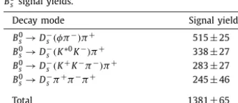
Table 1 B0
s signal yields.
Decay mode Signal yield
B0
s→D−s(φπ−)π+ 515±25
B0
s→D−s(K∗0K−)π+ 338±27
B0
s→D−s(K+K−π−)π+ 283±27
B0
s→D−sπ+π−π+ 245±46
Total 1381±65
Thebdecay backgrounds include partially reconstructed B0
s
de-cays, as well as fully and partially reconstructedB0and
Λ
bdecayswith one mis-identified daughter particle. Their shapes are derived from a large simulated event sample, where all selection cuts were applied on generator level quantities. The invariant mass spectra were then smeared with a Gaussian distribution to take into ac-count effects of detector resolution. This approach was validated by comparing the results with those from a full simulation includ-ing a detailed description of the detector response. The relative normalization factors for the differentbdecay backgrounds are pa-rameters in the fit. They are constrained to be the same for the threeB0s
→
D−sπ
+decay modes.The fit returns a value ofm
(
B0s)
=
5364.
7±
0.
7 MeV/
c2, about 1.
5 MeV/
c2 below the PDG value[8]. This mass shift is attributedto imperfections in the detector alignment and magnetic field cal-ibration. A dedicated study on the momentum scale resulted in a correction for this effect[10]. This calibration procedure is how-ever not used for the analysis presented here as the momentum scale correction largely cancels in the calculation of
ms. The mass
templates describingb decay backgrounds are shifted according to the observed bias. The fit gives signal mass resolutions of
σ
m=
18
.
1 MeV/
c2 for the B0s→
Ds−π
+ modes andσ
m=
12.
7 MeV/
c2for the B0s
→
D−sπ
+π
−π
+ mode, respectively. The signal yieldsextracted from the fit are summarized in Table 1. For the re-mainder of the analysis, the invariant B0s mass range is limited to
[
m(
B0s)
−
3σ
m,
5.
85 GeV/
c2]
and[
m(
B0s)
−
3σ
m,
5.
60 GeV/
c2]
fortheB0
s
→
D−sπ
+andB0s→
D−sπ
+π
−π
+modes, respectively. Thelower cut of this asymmetric mass window is chosen to reject all background candidates from partial reconstructed B0s decays. The only remainingbdecay backgrounds are thus due to mis-identified B0and
Λ
bdecays. The candidates in the high mass sidebands
pro-vide a clean sample of combinatorial background. Including them in the fit permits to determine the decay time distribution and tagging behaviour of this background contribution.
The parameters derived in the fit to the mass distributions are fixed for the remainder of the analysis.
4. Fit to the decay time distribution
Ignoring detector resolution effects, selection biases and flavour tagging, the distribution of the decay timet of the signal is de-scribed by
P
t(
t)
∝
Γ
se−ΓstcoshΓ
s2 t
θ (
t),
(2)where
Γ
s is the B0s decay width andΓ
sthe decay widthdiffer-ence between the heavy and the light mass eigenstates. In the fit
Γ
s is fixed to its PDG value of 0.
09Γ
s [8]. As part of theeval-uation of systematic uncertainties on
ms, the assumed value of
Γ
sis varied within its current uncertainty between 0 and 0.
2Γ
s.The step function
θ (
t)
restricts the PDF to positive decay times. The true decay time is convolved with the decay time res-olution function of the detector. An event-by-event estimate of the decay time resolution is calculated by the fitting algorithm,which reconstructs the decay vertex of the B0
s and computes its
decay length and decay time. No constraint on the D−s mass is applied in the computation of the decay time in order to mini-mize sensitivity to the knowledge of the momentum scale of the experiment. The decay time uncertainty calculated by the fitting algorithm does not include possible effects from an imperfect un-derstanding of the detector material or its spatial alignment. To correct for such effects, the calculated event-by-event decay time uncertainties,
σ
t, are multiplied by a constant scale factor Sσt. The value of Sσt is determined from data, using a sample of fake B0
s
candidates formed by a prompt D−s and a
π
+ from the primary vertex. The contamination due to secondary D−s from B decays is estimated and statistically subtracted using the measured D−s impact parameter distribution. The distribution of decay times for this fake B0s sample, each divided by its calculated event-by-event uncertainty, is fitted with a Gaussian function and Sσt is taken as the resulting standard deviation. Using the full sample of fake B0s
candidates, a value of Sσt
=
1.
3 is obtained. This value is used as the nominal scale factor in themsanalysis. Studying different
re-gions of phase space of the fake B0
s candidates separately, values
for Sσt between 1.2 and 1.4 are obtained. This variation is taken into account for evaluating the systematic uncertainties on
ms.
Including the nominal scale factor Sσt
=
1.
3, the average decay time resolution is 44 fs for the B0s
→
D−sπ
+ sample and 36 fs fortheB0s
→
D−sπ
+π
−π
+sample. The decay time resolution is taken into account in the PDF by convolving Eq. (2)with a Gaussian G with mean zero and standard deviation 1.
3σ
t.The shape of the decay time distribution is distorted by trigger and offline selection criteria which require several particles with large impact parameter with respect to the primary vertex. This is accounted for in the PDF by introducing an acceptance func-tion
(
t)
, derived from a full detector simulation. Determining(
t)
from simulation is deemed acceptable since it cancels to first or-der in the determination of
ms. The untagged signal decay time
PDF becomes
P
t(
t|
σ
t)
∝
Γ
se−ΓstcoshΓ
s2 t
θ (
t)
⊗
G(
t,
Sσtσ
t)
(
t).
(3)The decay time distributions for theb decay backgrounds from B0
and
Λ
b decays are described in the same way as that forsig-nal B0s candidates, using the PDG values for their lifetimes and
Γ
=
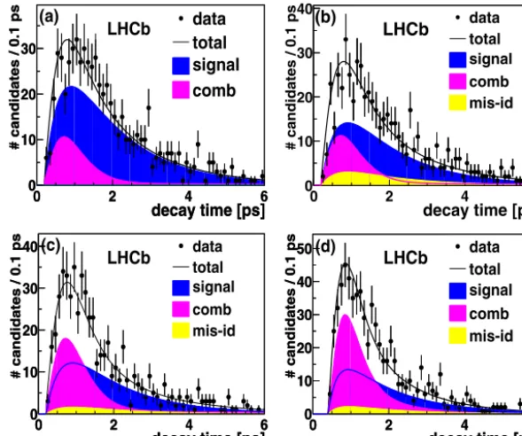
0. The shape of the decay time distribution for the com-binatorial background is described by the sum of two exponential functions multiplied by a second order polynomial. The parame-ters of these functions are derived from the high mass sidebands. Fig. 2 illustrates the results of the lifetime fit. Within its statisti-cal uncertainty the reconstructed B0s lifetime agrees with the PDG value[8].5. Flavour tagging
To determine the flavour of the B0
s candidate at production
180 LHCb Collaboration / Physics Letters B 709 (2012) 177–184
Fig. 2.Decay time distributions for (a)B0
s→D−s(φπ−)π+, (b)B0s→D−s(K∗0K−)π+, (c)B0s→D−s(K+K−π−)π+and (d)B0s→D−sπ+π−π+candidates. The data and the
fit projection are from a mass range of±3σmaround the reconstructedB0s mass. The abbreviations for the various fit components are introduced inFig. 1.
tagging particle and theB0
s candidate. The optimization of the
tag-ging algorithms and an initial calibration of
η
are performed in an independent analysis using large event samples of B→
μ
+D∗−X and B+→
J/ψ
K+ decays. More details on the individual tagging algorithms and this calibration procedure can be found in Ref.[11]. The B→
μ
+D∗−X and B+→
J/ψ
K+ events used in the optimization and calibration were collected using different trig-ger and selection criteria than for the B0s
→
D−sπ
+ and B0s→
D−s
π
+π
−π
+ events used in thems analysis described here. As
trigger and selection cuts can bias the distributions of the event properties used by the tagging algorithms, this could result in a biased estimate for the B0s
→
D−sπ
+ and B0s→
D−sπ
+π
−π
+events. Therefore, a re-calibration is performed using a sample of 6000 B0
→
D−π
+ events, which have a similar topology tothe B0s
→
D−sπ
+ and B0s→
D−sπ
+π
−π
+ events, and were col-lected using the same trigger and similar selection cuts. This event sample is used to perform a measurement of the B0–B0flavour oscillation using a very similar method to that described here. In that measurement the true event mistag probability,
ω
, is parameterized as a linear function ofη
using the relationshipω
(
η
)
=
a+
b×
(
η
−
η
)
, whereη
=
0.
3276 is the mean of the distribution of theη
values obtained from the initial tagger op-timization. The parametersa=
0.
311±
0.
022 and b=
0.
61±
0.
25 are determined as part of the maximum likelihood fit of theB0–B0oscillation signal and found to be consistent with the original calibration. As a by-product of this re-calibration procedure the B0–B0 oscillation frequency is measured. The resulting value of
md
=
0.
499±
0.
032(
stat)
±
0.
003(
syst)
ps−1, thoughstatisti-cally less precise, is in good agreement with the PDG value of
md
=
0.
507±
0.
004 ps−1[8]and provides a valuable cross checkof the procedure.
The statistical power of the tagging is determined by the “ef-fective” tagging efficiency for signal events and is defined as
eff
=
s
×
1
iWii
1
−
2ω
(
η
i)
2×
Wi,
(4)where the signal tagging efficiency
s is a free parameter in the
fit of the oscillation frequency described in the next section. Wi
is the probability for being a signal event as determined by the invariant mass and decay time PDFs. The index i runs over all B0
s
candidates.
6. Measurement of the oscillation frequency
To determine the oscillation frequency,
ms, the decay time
PDF for signal candidates with tagging information is modified in the following way:
P
t(
t,
q|
σ
t,
η
)
∝
Γ
se−Γst1 2
cosh
Γ
s2 t
+
q1−
2ω
(
η
)
cos(
mst)
θ (
t)
⊗
G(
t,
Sσtσ
t)
(
t)
s
.
(5) The decay time PDF for untagged signal events is given by Eq.(3) multiplied by an additional factor(
1−
s
)
. The calibrationpa-rameters a andb of the mistag probability
ω
(
η
)
are identical for all signal and b decay background components. Within Gaussian constraints they are set to the values found in the calibration de-scribed in the previous section. The signal tagging efficiencysfor
the B0s
→
D−sπ
+ andB0s→
D−sπ
+π
−π
+modes are two separate parameters in the fit. The same values ofs
are however used for signal and b decay background components in each of these two categories. In the description of the combinatorial background a separate parameter for the tagging efficiency is introduced for each of the four modes. In addition, tagging asymmetry parameters are introduced in the PDFs for the combinatorial background, to allow for a different number of events tagged asB0s orB0s in each mode.As expected the fit results for these asymmetries are compatible with zero.
The fit for the oscillation frequency
ms is performed
simul-taneously to all four B0
LHCb Collaboration / Physics Letters B 709 (2012) 177–184 181
Fig. 3.Likelihood scan formsin the range[0.0,25.0]ps−1. The line at−2lnL=
[image:6.612.326.551.100.165.2]20.9 indicates the value in the limitms= ∞.
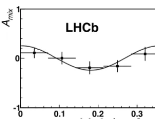
Fig. 4.Measured asymmetry forB0
s candidates in bins of the decay timetmodulo
2π/ms. The projection of the likelihood fit is superimposed.
0
.
11 ps−1 (statistical uncertainty only). Signal tagging efficiencies ofs
=
(
23.
6±
1.
3)
% ands
=
(
17.
6±
3.
2)
% are found for theB0s→
D−s
π
+andB0s→
D−sπ
+π
−π
+modes, respectively. The combined effective tagging efficiency for all four modes iseff
=
(
3.
8±
2.
1)
%. The likelihood profile as a function of the assumed oscillation fre-quencyms is shown in Fig. 3. The statistical significance of the
signal is evaluated to be 4
.
6σ
by comparing the likelihood value at the minimum of the fit with that found in the limitms
= ∞
.To illustrate the oscillation pattern, we define the time-depen-dent mixing asymmetry as
Amix(t
)
=
N+
(
t)
−
N−(
t)
N+
(
t)
+
N−(
t)
(6)whereN+
(
t)
andN−(
t)
are the number of background subtracted B0s signal candidates with a given decay time t and tagging de-cision+
1 and−
1, respectively. Note, that this definition of the asymmetry does not include any information on the mistag prob-abilities and therefore does not use the full information of the likelihood fit. Despite the limited size of the sample, the oscillation pattern is clearly visible when the asymmetry is plotted in bins of the decay time modulo 2π
/
ms (Fig. 4). In an ideal scenario ofperfect tagging and perfect decay time resolution the amplitude of this oscillation would be 1.0. The observed amplitude is reduced due to the performance of the tagging algorithm by a factor 0.41. Another reduction of 0.65 occurs due to the limited decay time resolution.
7. Systematic uncertainties
[image:6.612.92.248.228.348.2]The dominant source of systematic uncertainty is due to the knowledge of the absolute decay time scale of the experiment. This uncertainty is dominated by the knowledge of the z scale. A rel-ative uncertainty of 0.1% on the z scale and thus on the decay length is assigned based on comparisons of detector surveys and
Table 2
Summary of the systematic uncertainties onms. The total systematic
un-certainty is defined as the quadratic sum of the individual components.
Source Uncertainty [ps−1]
Momentum scale 0.004
zscale 0.018
Combinatorial background mass shape 0.010 Decay time resolution 0.006
Total systematic uncertainty 0.022
a software alignment using reconstructed tracks. This leads to a systematic uncertainty of 0.018 ps−1 on
ms. A second
contribu-tion to the decay time scale is due to the momentum scale of the experiment. From an independent analysis of the mass scale us-ing various known resonances an uncertainty of the uncalibrated momentum scale of less than 0.1% is estimated. This uncertainty partially cancels as it enters both the reconstructed B0s mass and theB0s momentum. The resulting relative uncertainty on the decay time is 0.02%, which translates to an absolute systematic uncer-tainty of 0.004 ps−1 on
m
s.
The next largest systematic uncertainty is related to the de-scription of the combinatorial background in the fit to the mass spectra. It is evaluated by replacing the exponential function by a first order polynomial. Based on the shift in the value obtained for
ms, a systematic uncertainty of 0.010 ps−1 is assigned. Finally,
based on variations of the decay time resolution scale factor Sσt within its estimated uncertainty from 1.2 to 1.4, a systematic un-certainty of 0.006 ps−1is assigned on
ms. These contributions to
the systematic uncertainty on
msare summarized inTable 2.
Various other possible sources of systematic effects have been studied, such as the decay time resolution model, the decay time acceptance, releasing parameters of the invariant mass and decay time PDF in the mixing fit, different parameterizations of the in-variant mass of the b decay backgrounds and variations of the value of
Γ
s. They are found to be negligible.8. Conclusion
A measurement of the B0
s–B0s oscillation frequency
ms is
per-formed using B0s
→
D−sπ
+ and B0s→
D−sπ
+π
−π
+ decays col-lected in 36 pb−1ofppcollisions at√
s=
7 TeV in 2010. The result is found to bems
=
17.
63±
0.
11(
stat)
±
0.
02(
syst)
ps−1.
(7)This is in good agreement with the previous best measurement of
ms
=
17.
77±
0.
10(
stat)
±
0.
07(
syst)
ps−1, reported by theCDF Collaboration [3]. As a by product of the analysis we also determine a value for the B0–B0 oscillation frequency
m
d
=
0
.
499±
0.
032(
stat)
±
0.
003(
syst)
ps−1. Our results are com-pletely dominated by statistical uncertainties and thus significant improvements are expected with larger data sets.Acknowledgements
182 LHCb Collaboration / Physics Letters B 709 (2012) 177–184
We also acknowledge the support received from the ERC under FP7 and the Region Auvergne.
Open access
This article is published Open Access at sciencedirect.com. It is distributed under the terms of the Creative Commons Attribu-tion License 3.0, which permits unrestricted use, distribuAttribu-tion, and reproduction in any medium, provided the original authors and source are credited.
References
[1] ARGUS Collaboration, H. Albrecht, et al., Phys. Lett. B 192 (1987) 245.
[2] D0 Collaboration, V.M. Abazov, et al., Phys. Rev. Lett. 97 (2006) 021802. [3] CDF Collaboration, A. Abulencia, et al., Phys. Rev. Lett. 97 (2006) 062003. [4] LHCb Collaboration, R. Aaij, et al., Measurement of the CP-violating phaseφsin
the decayB0
s→J/ψφ, Phys. Rev. Lett., in press, arXiv:1112.3183.
[5] LHCb Collaboration, A.A. Alves Jr., et al., JINST 3 (2008) S08005. [6] V.V. Gligorov, A single track HLT1 trigger, LHCb-PUB-2011-003. [7] M. Williams, et al., The HLT2 topological lines, LHCb-PUB-2011-002. [8] Particle Data Group, K. Nakamura, et al., J. Phys. G 37 (2010) 075021. [9] G. Punzi, Comments on likelihood fits with variable resolution, eConf C030908
WELT002, 2003.
[10] LHCb Collaboration, Measurement of b hadron masses with exclusive J/ψX
decays in 2010 data, LHCb-CONF-2011-027.
[11] LHCb Collaboration, Optimization and calibration of the LHCb flavour tagging performance using 2010 data, LHCb-CONF-2011-003;
LHCb Collaboration, R. Aaij, et al., Flavour tagging of B mesons at LHCb, in preparation; to be submitted to Eur. J. Phys. C, LHCb-PAPER-2011-027.
LHCb Collaboration
R. Aaij
23, B. Adeva
36, M. Adinolfi
42, C. Adrover
6, A. Affolder
48, Z. Ajaltouni
5, J. Albrecht
37, F. Alessio
37,
M. Alexander
47, G. Alkhazov
29, P. Alvarez Cartelle
36, A.A. Alves Jr.
22, S. Amato
2, Y. Amhis
38,
J. Anderson
39, R.B. Appleby
50, O. Aquines Gutierrez
10, F. Archilli
18,
37, L. Arrabito
53, A. Artamonov
34,
M. Artuso
52,
37, E. Aslanides
6, G. Auriemma
22,
m, S. Bachmann
11, J.J. Back
44, D.S. Bailey
50,
V. Balagura
30,
37, W. Baldini
16, R.J. Barlow
50, C. Barschel
37, S. Barsuk
7, W. Barter
43, A. Bates
47,
C. Bauer
10, Th. Bauer
23, A. Bay
38, I. Bediaga
1, K. Belous
34, I. Belyaev
30,
37, E. Ben-Haim
8,
M. Benayoun
8, G. Bencivenni
18, S. Benson
46, J. Benton
42, R. Bernet
39, M.-O. Bettler
17,
M. van Beuzekom
23, A. Bien
11, S. Bifani
12, A. Bizzeti
17,
h, P.M. Bjørnstad
50, T. Blake
49, F. Blanc
38,
C. Blanks
49, J. Blouw
11, S. Blusk
52, A. Bobrov
33, V. Bocci
22, A. Bondar
33, N. Bondar
29, W. Bonivento
15,
S. Borghi
47, A. Borgia
52, T.J.V. Bowcock
48, C. Bozzi
16, T. Brambach
9, J. van den Brand
24, J. Bressieux
38,
D. Brett
50, S. Brisbane
51, M. Britsch
10, T. Britton
52, N.H. Brook
42, H. Brown
48, A. Büchler-Germann
39,
I. Burducea
28, A. Bursche
39, J. Buytaert
37, S. Cadeddu
15, J.M. Caicedo Carvajal
37, O. Callot
7, M. Calvi
20,
j,
M. Calvo Gomez
35,
n, A. Camboni
35, P. Campana
18,
37, A. Carbone
14, G. Carboni
21,
k, R. Cardinale
19,
37,
i,
A. Cardini
15, L. Carson
36, K. Carvalho Akiba
23, G. Casse
48, M. Cattaneo
37, M. Charles
51,
Ph. Charpentier
37, N. Chiapolini
39, K. Ciba
37, X. Cid Vidal
36, G. Ciezarek
49, P.E.L. Clarke
46,
37,
M. Clemencic
37, H.V. Cliff
43, J. Closier
37, C. Coca
28, V. Coco
23, J. Cogan
6, P. Collins
37, F. Constantin
28,
G. Conti
38, A. Contu
51, A. Cook
42, M. Coombes
42, G. Corti
37, G.A. Cowan
38, R. Currie
46, B. D’Almagne
7,
C. D’Ambrosio
37, P. David
8, I. De Bonis
4, S. De Capua
21,
k, M. De Cian
39, F. De Lorenzi
12,
J.M. De Miranda
1, L. De Paula
2, P. De Simone
18, D. Decamp
4, M. Deckenhoff
9, H. Degaudenzi
38,
37,
M. Deissenroth
11, L. Del Buono
8, C. Deplano
15, O. Deschamps
5, F. Dettori
15,
d, J. Dickens
43,
H. Dijkstra
37, P. Diniz Batista
1, S. Donleavy
48, A. Dosil Suárez
36, D. Dossett
44, A. Dovbnya
40,
F. Dupertuis
38, R. Dzhelyadin
34, C. Eames
49, S. Easo
45, U. Egede
49, V. Egorychev
30, S. Eidelman
33,
D. van Eijk
23, F. Eisele
11, S. Eisenhardt
46, R. Ekelhof
9, L. Eklund
47, Ch. Elsasser
39, D.G. d’Enterria
35,
o,
D. Esperante Pereira
36, L. Estève
43, A. Falabella
16,
e, E. Fanchini
20,
j, C. Färber
11, G. Fardell
46,
C. Farinelli
23, S. Farry
12, V. Fave
38, V. Fernandez Albor
36, M. Ferro-Luzzi
37, S. Filippov
32,
C. Fitzpatrick
46, M. Fontana
10, F. Fontanelli
19,
i, R. Forty
37, M. Frank
37, C. Frei
37, M. Frosini
17,
37,
f,
S. Furcas
20, A. Gallas Torreira
36, D. Galli
14,
c, M. Gandelman
2, P. Gandini
51, Y. Gao
3, J.-C. Garnier
37,
J. Garofoli
52, J. Garra Tico
43, L. Garrido
35, C. Gaspar
37, N. Gauvin
38, M. Gersabeck
37, T. Gershon
44,
37,
Ph. Ghez
4, V. Gibson
43, V.V. Gligorov
37, C. Göbel
54, D. Golubkov
30, A. Golutvin
49,
30,
37, A. Gomes
2,
H. Gordon
51, M. Grabalosa Gándara
35, R. Graciani Diaz
35, L.A. Granado Cardoso
37, E. Graugés
35,
G. Graziani
17, A. Grecu
28, S. Gregson
43, B. Gui
52, E. Gushchin
32, Yu. Guz
34, T. Gys
37, G. Haefeli
38,
C. Haen
37, S.C. Haines
43, T. Hampson
42, S. Hansmann-Menzemer
11,
∗
, R. Harji
49, N. Harnew
51,
J. Harrison
50, P.F. Harrison
44, J. He
7, V. Heijne
23, K. Hennessy
48, P. Henrard
5, J.A. Hernando Morata
36,
E. van Herwijnen
37, E. Hicks
48, W. Hofmann
10, K. Holubyev
11, P. Hopchev
4, W. Hulsbergen
23,
LHCb Collaboration / Physics Letters B 709 (2012) 177–184 183
P. Koppenburg
23, A. Kozlinskiy
23, L. Kravchuk
32, K. Kreplin
11, M. Kreps
44, G. Krocker
11, P. Krokovny
11,
F. Kruse
9, K. Kruzelecki
37, M. Kucharczyk
20,
25,
37, S. Kukulak
25, R. Kumar
14,
37, T. Kvaratskheliya
30,
37,
V.N. La Thi
38, D. Lacarrere
37, G. Lafferty
50, A. Lai
15, D. Lambert
46, R.W. Lambert
37, E. Lanciotti
37,
G. Lanfranchi
18, C. Langenbruch
11, T. Latham
44, R. Le Gac
6, J. van Leerdam
23, J.-P. Lees
4, R. Lefèvre
5,
A. Leflat
31,
37, J. Lefrançois
7, O. Leroy
6, T. Lesiak
25, L. Li
3, L. Li Gioi
5, M. Lieng
9, M. Liles
48,
R. Lindner
37, C. Linn
11, B. Liu
3, G. Liu
37, J.H. Lopes
2, E. Lopez Asamar
35, N. Lopez-March
38, J. Luisier
38,
F. Machefert
7, I.V. Machikhiliyan
4,
30, F. Maciuc
10, O. Maev
29,
37, J. Magnin
1, S. Malde
51,
R.M.D. Mamunur
37, G. Manca
15,
d, G. Mancinelli
6, N. Mangiafave
43, U. Marconi
14, R. Märki
38,
J. Marks
11, G. Martellotti
22, A. Martens
7, L. Martin
51, A. Martín Sánchez
7, D. Martinez Santos
37,
A. Massafferri
1, Z. Mathe
12, C. Matteuzzi
20, M. Matveev
29, E. Maurice
6, B. Maynard
52,
A. Mazurov
32,
16,
37, G. McGregor
50, R. McNulty
12, C. Mclean
14, M. Meissner
11, M. Merk
23, J. Merkel
9,
R. Messi
21,
k, S. Miglioranzi
37, D.A. Milanes
13,
37, M.-N. Minard
4, S. Monteil
5, D. Moran
12,
P. Morawski
25, R. Mountain
52, I. Mous
23, F. Muheim
46, K. Müller
39, R. Muresan
28,
38, B. Muryn
26,
M. Musy
35, J. Mylroie-Smith
48, P. Naik
42, T. Nakada
38, R. Nandakumar
45, J. Nardulli
45, I. Nasteva
1,
M. Nedos
9, M. Needham
46, N. Neufeld
37, C. Nguyen-Mau
38,
p, M. Nicol
7, S. Nies
9, V. Niess
5,
N. Nikitin
31, A. Oblakowska-Mucha
26, V. Obraztsov
34, S. Oggero
23, S. Ogilvy
47, O. Okhrimenko
41,
R. Oldeman
15,
d, M. Orlandea
28, J.M. Otalora Goicochea
2, P. Owen
49, B. Pal
52, J. Palacios
39,
M. Palutan
18, J. Panman
37, A. Papanestis
45, M. Pappagallo
13,
b, C. Parkes
47,
37, C.J. Parkinson
49,
G. Passaleva
17, G.D. Patel
48, M. Patel
49, S.K. Paterson
49, G.N. Patrick
45, C. Patrignani
19,
i,
C. Pavel-Nicorescu
28, A. Pazos Alvarez
36, A. Pellegrino
23, G. Penso
22,
l, M. Pepe Altarelli
37,
S. Perazzini
14,
c, D.L. Perego
20,
j, E. Perez Trigo
36, A. Pérez-Calero Yzquierdo
35, P. Perret
5,
M. Perrin-Terrin
6, G. Pessina
20, A. Petrella
16,
37, A. Petrolini
19,
i, B. Pie Valls
35, B. Pietrzyk
4, T. Pilar
44,
D. Pinci
22, R. Plackett
47, S. Playfer
46, M. Plo Casasus
36, G. Polok
25, A. Poluektov
44,
33, E. Polycarpo
2,
D. Popov
10, B. Popovici
28, C. Potterat
35, A. Powell
51, T. du Pree
23, J. Prisciandaro
38, V. Pugatch
41,
A. Puig Navarro
35, W. Qian
52, J.H. Rademacker
42, B. Rakotomiaramanana
38, M.S. Rangel
2, I. Raniuk
40,
G. Raven
24, S. Redford
51, M.M. Reid
44, A.C. dos Reis
1, S. Ricciardi
45, K. Rinnert
48, D.A. Roa Romero
5,
P. Robbe
7, E. Rodrigues
47, F. Rodrigues
2, P. Rodriguez Perez
36, G.J. Rogers
43, S. Roiser
37,
V. Romanovsky
34, J. Rouvinet
38, T. Ruf
37, H. Ruiz
35, G. Sabatino
21,
k, J.J. Saborido Silva
36, N. Sagidova
29,
P. Sail
47, B. Saitta
15,
d, C. Salzmann
39, M. Sannino
19,
i, R. Santacesaria
22, R. Santinelli
37, E. Santovetti
21,
k,
M. Sapunov
6, A. Sarti
18,
l, C. Satriano
22,
m, A. Satta
21, M. Savrie
16,
e, D. Savrina
30, P. Schaack
49,
M. Schiller
11, S. Schleich
9, M. Schmelling
10, B. Schmidt
37, O. Schneider
38, A. Schopper
37,
M.-H. Schune
7, R. Schwemmer
37, A. Sciubba
18,
l, M. Seco
36, A. Semennikov
30, K. Senderowska
26,
I. Sepp
49, N. Serra
39, J. Serrano
6, P. Seyfert
11, B. Shao
3, M. Shapkin
34, I. Shapoval
40,
37, P. Shatalov
30,
Y. Shcheglov
29, T. Shears
48, L. Shekhtman
33, O. Shevchenko
40, V. Shevchenko
30, A. Shires
49,
R. Silva Coutinho
54, H.P. Skottowe
43, T. Skwarnicki
52, A.C. Smith
37, N.A. Smith
48, K. Sobczak
5,
F.J.P. Soler
47, A. Solomin
42, F. Soomro
49, B. Souza De Paula
2, B. Spaan
9, A. Sparkes
46, P. Spradlin
47,
F. Stagni
37, S. Stahl
11, O. Steinkamp
39, S. Stoica
28, S. Stone
52,
37, B. Storaci
23, M. Straticiuc
28,
U. Straumann
39, N. Styles
46, V.K. Subbiah
37, S. Swientek
9, M. Szczekowski
27, P. Szczypka
38,
T. Szumlak
26, S. T’Jampens
4, E. Teodorescu
28, F. Teubert
37, C. Thomas
51,
45, E. Thomas
37,
J. van Tilburg
11, V. Tisserand
4, M. Tobin
39, S. Topp-Joergensen
51, M.T. Tran
38, A. Tsaregorodtsev
6,
N. Tuning
23, A. Ukleja
27, P. Urquijo
52, U. Uwer
11, V. Vagnoni
14, G. Valenti
14, R. Vazquez Gomez
35,
P. Vazquez Regueiro
36, S. Vecchi
16, J.J. Velthuis
42, M. Veltri
17,
g, K. Vervink
37, B. Viaud
7, I. Videau
7,
X. Vilasis-Cardona
35,
n, J. Visniakov
36, A. Vollhardt
39, D. Voong
42, A. Vorobyev
29, H. Voss
10, K. Wacker
9,
S. Wandernoth
11, J. Wang
52, D.R. Ward
43, A.D. Webber
50, D. Websdale
49, M. Whitehead
44,
D. Wiedner
11, L. Wiggers
23, G. Wilkinson
51, M.P. Williams
44,
45, M. Williams
49, F.F. Wilson
45,
J. Wishahi
9, M. Witek
25,
37, W. Witzeling
37, S.A. Wotton
43, K. Wyllie
37, Y. Xie
46, F. Xing
51, Z. Yang
3,
R. Young
46, O. Yushchenko
34, M. Zavertyaev
10,
a, L. Zhang
52, W.C. Zhang
12, Y. Zhang
3, A. Zhelezov
11,
L. Zhong
3, E. Zverev
31, A. Zvyagin
371Centro Brasileiro de Pesquisas Físicas (CBPF), Rio de Janeiro, Brazil 2Universidade Federal do Rio de Janeiro (UFRJ), Rio de Janeiro, Brazil 3Center for High Energy Physics, Tsinghua University, Beijing, China 4LAPP, Université de Savoie, CNRS/IN2P3, Annecy-Le-Vieux, France
184 LHCb Collaboration / Physics Letters B 709 (2012) 177–184
7LAL, Université Paris-Sud, CNRS/IN2P3, Orsay, France
8LPNHE, Université Pierre et Marie Curie, Université Paris Diderot, CNRS/IN2P3, Paris, France 9Fakultät Physik, Technische Universität Dortmund, Dortmund, Germany
10Max-Planck-Institut für Kernphysik (MPIK), Heidelberg, Germany
11Physikalisches Institut, Ruprecht-Karls-Universität Heidelberg, Heidelberg, Germany 12School of Physics, University College Dublin, Dublin, Ireland
13Sezione INFN di Bari, Bari, Italy 14Sezione INFN di Bologna, Bologna, Italy 15Sezione INFN di Cagliari, Cagliari, Italy 16Sezione INFN di Ferrara, Ferrara, Italy 17Sezione INFN di Firenze, Firenze, Italy
18Laboratori Nazionali dell’INFN di Frascati, Frascati, Italy 19Sezione INFN di Genova, Genova, Italy
20Sezione INFN di Milano Bicocca, Milano, Italy 21Sezione INFN di Roma Tor Vergata, Roma, Italy 22Sezione INFN di Roma La Sapienza, Roma, Italy
23Nikhef National Institute for Subatomic Physics, Amsterdam, Netherlands
24Nikhef National Institute for Subatomic Physics and Vrije Universiteit, Amsterdam, Netherlands 25Henryk Niewodniczanski Institute of Nuclear Physics, Polish Academy of Sciences, Cracow, Poland 26Faculty of Physics & Applied Computer Science, Cracow, Poland
27Soltan Institute for Nuclear Studies, Warsaw, Poland
28Horia Hulubei National Institute of Physics and Nuclear Engineering, Bucharest-Magurele, Romania 29Petersburg Nuclear Physics Institute (PNPI), Gatchina, Russia
30Institute of Theoretical and Experimental Physics (ITEP), Moscow, Russia 31Institute of Nuclear Physics, Moscow State University (SINP MSU), Moscow, Russia 32Institute for Nuclear Research of the Russian Academy of Sciences (INR RAN), Moscow, Russia 33Budker Institute of Nuclear Physics (SB RAS) and Novosibirsk State University, Novosibirsk, Russia 34Institute for High Energy Physics (IHEP), Protvino, Russia
35Universitat de Barcelona, Barcelona, Spain
36Universidad de Santiago de Compostela, Santiago de Compostela, Spain 37European Organization for Nuclear Research (CERN), Geneva, Switzerland 38Ecole Polytechnique Fédérale de Lausanne (EPFL), Lausanne, Switzerland 39Physik-Institut, Universität Zürich, Zürich, Switzerland
40NSC Kharkiv Institute of Physics and Technology (NSC KIPT), Kharkiv, Ukraine 41Institute for Nuclear Research of the National Academy of Sciences (KINR), Kyiv, Ukraine 42H.H. Wills Physics Laboratory, University of Bristol, Bristol, United Kingdom
43Cavendish Laboratory, University of Cambridge, Cambridge, United Kingdom 44Department of Physics, University of Warwick, Coventry, United Kingdom 45STFC Rutherford Appleton Laboratory, Didcot, United Kingdom
46School of Physics and Astronomy, University of Edinburgh, Edinburgh, United Kingdom 47School of Physics and Astronomy, University of Glasgow, Glasgow, United Kingdom 48Oliver Lodge Laboratory, University of Liverpool, Liverpool, United Kingdom 49Imperial College London, London, United Kingdom
50School of Physics and Astronomy, University of Manchester, Manchester, United Kingdom 51Department of Physics, University of Oxford, Oxford, United Kingdom
52Syracuse University, Syracuse, NY, United States 53CC-IN2P3, CNRS/IN2P3, Lyon-Villeurbanne, Franceq
54Pontifícia Universidade Católica do Rio de Janeiro (PUC-Rio), Rio de Janeiro, Brazilr
*
Corresponding author.E-mail address:[email protected](S. Hansmann-Menzemer).
a P.N. Lebedev Physical Institute, Russian Academy of Science (LPI RAS), Moscow, Russia. b Università di Bari, Bari, Italy.
c Università di Bologna, Bologna, Italy. d Università di Cagliari, Cagliari, Italy. e Università di Ferrara, Ferrara, Italy. f Università di Firenze, Firenze, Italy. g Università di Urbino, Urbino, Italy.
h Università di Modena e Reggio Emilia, Modena, Italy. i
Università di Genova, Genova, Italy.
j Università di Milano Bicocca, Milano, Italy. k Università di Roma Tor Vergata, Roma, Italy.
l Università di Roma La Sapienza, Roma, Italy. m Università della Basilicata, Potenza, Italy.
n LIFAELS, La Salle, Universitat Ramon Llull, Barcelona, Spain.
o Institució Catalana de Recerca i Estudis Avançats (ICREA), Barcelona, Spain. p Hanoi University of Science, Hanoi, Viet Nam.
q Associated member.