Poisson-Fermi Modeling of Ion Activities in Aqueous Single and Mixed Electrolyte Solutions at Variable Temperature

arXiv:1801.03470v1 [cond-mat.soft] 23 Dec 2017

Mixed Electrolyte Solutions at Variable Temperature

Jinn-Liang Liu

Institute of Computational and Modeling Science, National Tsing Hua University, Hsinchu 300,

Taiwan. E-mail: [email protected]

Bob Eisenberg

Department of Applied Mathematics, Illinois Institute of Technology, Chicago IL 60616. USA

(Dated: January 11, 2018)

Abstract. The combinatorial explosion of empirical parameters in tens of thousands

presents a tremendous challenge for extended Debye-H¨uckel models to calculate activity

coefficients of aqueous mixtures of most important salts in chemistry. The explosion of

pa-rameters originates from the phenomenological extension of the Debye-H¨uckel theory that

does not take steric and correlation effects of ions and water into account. In contrast, the

Poisson-Fermi theory developed in recent years treats ions and water molecules as

nonuni-form hard spheres of any size with interstitial voids and includes ion-water and ion-ion

correlations. We present a Poisson-Fermi model and numerical methods for calculating the

individual or mean activity coefficient of electrolyte solutions with any arbitrary number of

ionic species in a large range of salt concentrations and temperatures. For each

activity-concentration curve, we show that the Poisson-Fermi model requires only three unchanging

parameters at most to well fit the corresponding experimental data. The three parameters

are associated with the Born radius of the solvation energy of an ion in electrolyte solution

that changes with salt concentrations in a highly nonlinear manner.

1. INTRODUCTION

Thermodynamic modeling of aqueous electrolyte solutions plays an important role in

chemical and biological sciences [1–13]. Despite intense efforts in the past century, robust

re-mains a remote ambition in the extended Debye-H¨uckel (DH) models due to the enormous

number of parameters that need to be adjusted, carefully and often subjectively [11, 13].

For example, the Pitzer model requires 8 parameters for a ternary system and up to 8

tem-perature coefficients (parameters) for every Pitzer parameter in a temtem-perature interval from

0 to about 200◦

C [11, 13]. It is indeed a frustrating despair (frustration on p. 11 in [9] and

despair on p. 301 in [1]) that approximately 22,000 parameters for combinatorial solutions of the most important 28 cations and 16 anions in salt chemistry have to be extracted from

the available experimental data for one temperature [11]. The Pitzer model is still the most

widely used DH model with unmatched precision for modeling aqueous electrolyte solutions

over wide ranges of composition, temperature, and pressure [13].

The Pitzer model and its variants [13] are all derived from the Debye-H¨uckel theory [14]

that in turn is based on a linear Poisson-Boltzmann (PB) equation [5] although potentials

calculated from PB near ions (for example) are often far beyond the linear range of the

po-tential near ions or interfaces. The PB equation treats ions as point charges without steric

volumes and water molecules as a homogeneous dielectric medium without steric volumes

either and with a constant dielectric constant that neglects ion-water and ion-ion

correla-tions. These simplifications give rise to the elegant, simple, and useful DH theory. However,

it is precisely because of the linearization and simplifications on steric and correlation effects

that extended DH models have needed an explosion in the number of parameters in order to

overcome the deficiencies (simplifications) of the classical Poisson-Boltzmann theory. The

nonlinear PB equation was developed by Gouy and Chapman [15, 16].

In the past few years, we have intensively investigated these two effects in a range of areas

from electric double layers [17, 18], ion activities [19], to biological ion channels [18, 20–24]

and consequently developed an advanced theory — the Poisson-Fermi (PF) theory — that

treats ions and water molecules as nonuniform hard spheres of any size with interstitial voids

and includes many of the correlation effects of ions and water. We refer to our previous

papers and references therein for a historical account of the literature of this theory. In [19],

we proposed a PF model for calculating activity coefficients of individual ions in aqueous

single NaCl and CaCl2 electrolyte solutions at the temperature 298.15 K. The model is

further tested in this paper for eight 1:1 electrolytes (LiCl, LiBr, NaF, NaCl, NaBr, KF,

KCl, and KBr), six 2:1 electrolytes (MgCl2, MgBr2, CaCl2, CaBr2, BaCl2, and BaBr2), one

298.15 to 573.15 K, and one 2:1 electrolyte (MgCl2) at various temperatures from 298.15 to

523.15 K, for which the experimental data were compiled by Valisk´o and Boda in [25] and

Rowland et al. in [13] from various experimental sources in [26–35].

The PF model is developed to calculate individual ion activities for which experimental

measurements and determination [10, 36, 37], interpretation of measurement data [26, 37–

39], and comparison of different experimental methods [37, 40] have been extensively

in-vestigated by Wilczek-Vera, Rodil, and Vera in the past two decades. PF results on mean

activity coefficients can be compared with experimental measurements using the

Debye-H¨uckel equation of individual ion activities [5].

In contrast to the Pitzer model, we show that all experimental data sets of individual

or mean activity coefficients as a function of variable concentration in single electrolytes or

mixtures at various temperatures can be well fitted by the PF model with only 3 parameters

at most for each activity-concentration data curve. The model is characterized by three

different domains, namely, the Born ion, hydration shell, and remaining solvent domains in

which the Born ion domain is most crucial because all activities around an ion are mainly

governed by the singular charge of the ion located at the center of the domain. The Born

ion domain is defined by the Born radius of the solvated ion, which is unknown and changes

with salt concentrations in a highly nonlinear manner.

The three parameters characterize three orders of approximation of the Born radius in

terms of ionic concentrations. Parameter 1 describes a correction of the experimental Born

radius of a single ion in pure water without any other ions. Parameter 2 describes an

adjustment of the unknown Born radius in electrolyte solution that accounts for the Debye

screening effect, which is proportional to the square root of the ionic strength of the solution.

Parameter 3 is an adjustment in the next order approximation beyond the DH treatment

of ionic atmosphere. The physical origin of these parameters is clear unlike that of most

parameters in the Pitzer method [11, 41]. It may even be possible in later work to calculate

some of these parameters from more detailed versions of our model.

Our approach to partition the free energy domain of a solvated ion into the above three

domains yields a better approximation to calculate the free energy since these

sub-domains are determined by the experimental data of solvation and thus separate short- and

long-range interactions of the ion in a more accurate way. This approach nevertheless incurs

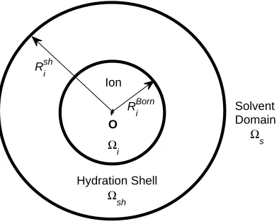
O Ion

Ω_i

Solvent Domain

Ω

s

Rsh_i

RBorn_i

Hydration Shell

Ω_sh

FIG. 1: The model domain Ω is partitioned into the ion domain Ωi (with radius R_iBorn), the

hydration shell domain Ωsh (with radius Rshi ), and the remaining solvent domain Ωs.

of the PF model in different domains with suitable interface conditions [17]. We therefore

present numerical methods in detail for future verification and development of the present

work.

2. THEORY

For an aqueous electrolyte solution with K species of ions, the Poisson-Fermi theory

proposed in [18, 21] treats all ions and water of any diameter as nonuniform hard spheres

with interstitial voids between these spheres. The activity coefficient γi of an ion of species

i in the solution describes the deviation of the chemical potential of the ion from ideality

(γi = 1). The excess chemical potential µexi =kBTlnγi can be calculated by [19, 42]

µex_i = ∆Gi−∆G0i, ∆Gi =

1

2qiφ(0), ∆G 0

i =

1 2qiφ

0_{(0), (1)}

where kB is the Boltzmann constant, T is an absolute temperature, qi is the ionic charge of

the hydrated ion (also denoted byi), φ(r) is a potential function of spatial variable r in the

domain Ω = Ωi∪Ωsh∪Ωs shown in Fig. 1, Ωi is the spherical domain occupied by the ioni,

the center (set to the origin) of the ion, φ(0) is the value of φ(r) at r = 0, and φ0_{(r) is a}

potential function when the solvent domain Ωs does not contain any ions at all with pure

water only. The potential functionφ(r) can be found by solving the Poisson-Fermi equation

[18]

l_c2_∇2₋1_{∇ ·}ǫ(r)_∇φ(r) =ρ(r), (2)

ǫ(r) =

  

ǫs=ǫwǫ0 in Ωsh∪Ωs

ǫi =ǫionǫ0 in Ωi

, lc =   

2aj in Ωsh∪Ωs

0 in Ωi

, (3)

ρ(r) =

        

ρs(r) = PK_k=1qkCk(r) in Ωs

0 in Ωsh

ρi(r) =qiδ(r−0) in Ωi

, (4)

Ck(r) =CkBexp

−βkφ(r) +

vk

v0S trc_(r)

in Ω, (5)

Strc_{(r) = ln}

Γ(r) ΓB

in Ω, (6)

where ǫ0 is the vacuum permittivity, ǫw is the dielectric constant of bulk water, ǫion is a

dielectric constant in Ωi, aj is the radius of a counterion of the ion i, and δ(r−0) is the

delta function at the origin.

The concentration functionCk(r) is described by a Fermi distribution (5), where CkB is a

constant bulk concentration for all k = 1,_{· · ·} , K+ 1, qK+1 = 0, βk =qk/kBT, vk = 4πa3k/3,

v0 =PKk=1+1vk

/(K+1) an average volume of all kinds of hard spheres,Strc_{(r) is called the}

steric potential, ΓB _{= 1−}PK+1

k=1 vkCkB is a constant void fraction, Γ(r) = 1− PK+1

k=1 vkCk(r) is a void fraction function, andK+ 1 denotes water. The radii of Ωi and the outer boundary

of Ωsh are denoted by RiBorn and Rshi , respectively, whose values will be determined by

experimental data. It is natural to choose the Born radius RBorn

i (not the ionic radius ai)

as the radius of Ωi [42]. We consider both first and second shells of the ion [43, 44].

The potential φ0_{(r) (in Eq. (1)) of the ideal system is obtained by setting ρ}

s(r) = 0 in

(4), i.e., all particles in Ωs do not electrostatically interact with each other since qk = 0 for

all k. The domain Ω is chosen to be sufficiently large so that φ(r) = 0 on the boundary

of the domain ∂Ω. The ideal potential φ0_{(r) is then a constant, i.e., ∆G}0

i is a constant

reference chemical potential independent of CB

k.

The distribution (5) is of Fermi type since all concentration functions have an upper

φ(r) at any location rin the domain Ω [21]. The Poisson-Fermi equation (2) and the Fermi

distribution (5) reduce to the Poisson-Boltzmann equation and the Boltzmann distribution

when lc = Strc = 0, i.e., when the correlation and steric effects are not considered. The

Boltzmann distribution Ck(r) = CkBexp (−βkφ(r)) would however diverge if φ(r) tends to

infinity. This is a major deficiency of PB theory for modeling a system with strong local

electric fields or interactions [45]. If the correlation length lc 6= 0, the dielectric operator

bǫ=ǫs(1−l2c∇2) in Eq. (2) approximates the permittivity of the bulk solvent and the linear

response of correlated ions [17, 20, 46, 47], and yields a dielectric function_eǫ(r) as an output

of solving Eq. (2) [21]. The exact value of_eǫ(r) at any r_∈Ωsh∪Ωs cannot be obtained from

Eq. (2) but can be approximated by the simple formula _eǫ(r)_≈ ǫi+ CH2O(r)(ǫs− ǫi)/C

B H2O

since the water density function CH2O(r) = CK+1(r) is an output of Eq. (5). This formula

is only for visualizing (approximately) the profile of_bǫor_eǫ. It is not an input of calculation.

The input is the correlation length lc in Eq. (3) [17, 20, 46, 47]. The actual outputs are the

numerical solutions of the partial differential equations and boundary conditions.

The factorvk/v0 multiplying the steric potential functionStrc(r) in Eq. (5) is a

modifica-tion of the unity used in our previous work [19, 21]. The steric energy₋vk

v0S

trc_(r)k

BT [21, 24]

of a typek particle depends not only on the voidness (Γ(r)) (or equivalently crowding) at r

but also on the volume vk of the particle itself. If all vk are equal (and thus vk =v0), then

all particle species at any location r _∈ Ωsh ∪Ωs have the same steric energy, i.e., uniform

particles are indistinguishable in steric energy. The steric potential is a mean-field

approxi-mation of Lennard-Jones (L-J) potentials that describe local variations of L-J distances (and

thus empty voids) between any pair of particles. L-J potentials are highly oscillatory and

extremely expensive and unstable to compute numerically [21]. Calculations that involve

L-J potentials, or even truncated versions of L-J potentials must be extensively checked to

be sure that results do not depend on irrelevant parameters.

3. METHODS

To avoid large errors in approximation caused by the delta function δ(r₋0) in (4), the

potential function can be decomposed as [17, 48, 49]

φ(r) =

  

e

φ(r) +φ∗

(r) +φL_{(r) in Ω}

i e

φ(r) in Ωsh∪Ωs

where φ∗

(r) = qi/(4πǫi|r−0|) and φe(r) is found by solving

l2_c∇2₋1_{∇ ·}ǫs∇φe(r) = ρ(r) in Ωsh∪Ωs (8)

−∇ ·ǫi∇φe(r) = 0 in Ωi (9)

without the singular source term ρi(r) =qiδ(r−0) and with the interface conditions 

  h

e

φ(r)i = 0

h

ǫ(r)_∇φe(r)_·ni =ǫi∇ φ∗(r) +φL(r))·n

for all r_∈ ∂Ωi, (10)

where n is an outward normal unit vector at r _∈ ∂Ωi and the jump function [u(r)] =

lim_rsh→_ru(rsh)−lim_ri→_ru(ri) with rsh∈ Ωsh and ri ∈Ωi [17]. The potential functionφ L_(r)

is the solution of the Laplace equation

∇2φL(r) = 0 in Ωi (11)

with the boundary condition

φL(r) = φ∗

(r) on ∂Ωi. (12)

The evaluation of the Green’s function φ∗

(r) on∂Ωi always yields finite numbers and thus

avoids the singularity in the solution process. The desired solvation energy ∆Gi in Eq. (1)

(and thus the individual ionic activity coefficient γi) is then evaluated by [17, 49]

∆Gi =kBT lnγi=

1 2qi

h e

φ(0) +φL(0)i. (13)

Since the interface ∂Ωi is a sphere centered at the origin, the Laplace potential φL(r) =

qi/(4πǫiRBorni ) is a constant in Ωi, i.e., Eq. (11) has been exactly solved.

The Poisson-Fermi equation (8) is a nonlinear fourth-order partial differential equation

(PDE) in Ωs. Newton’s iterative method is usually used for solving nonlinear problems. We

seek a sequence of approximate solutions nφem(r)

oM

m=1 by iteratively solving the linearized PF equation

l2_c∇2₋1_{∇ ·}ǫ_∇φem −ρ′s(φem−1)φem =ρs(φem−1)−ρ ′

s(φem−1) φem−1 in Ωs, (14)

until a tolerable potential functionφeM is reached, where φ0e (r) is a given initial guess

poten-tial function, ρs(φem−₁) =

PK

k=1qkCm

−₁

k (r), Cm

−₁

k (r) = CkBexp

−βkφem−₁(r) +

vk

v0S

trc

m−₁(r)

,

Strc

m−1(r) = ln

_Γ

0(r)

ΓB

, Γm−₁(r) = 1−

PK+1

k=1 vkCm

−1

k (r), ρ

′

s(φem−₁) =

PK

k=1(−βkqk)Cm

−1

and ρ′

s(φe) = _ddφeρs(φe). Note that the differentiation in ρ

′

s(φe) is performed only with respect

toφewhereas Strc _{is treated as another independent variable although S}trc _{depends on φ}e_as

well. Therefore, ρ′

s(φe) is not exact implying that this is an inexact Newton’s method [50].

The fourth-order problem can be resolved by transforming Eq. (14) into two second-order

PDEs [17]

ǫs l2c∇2 −1

Ψ(r) = ρ(φem−₁) in Ω_sh∪Ω_s (15)

−ǫs∇2φem(r)−ρ′(φem−1) φem(r) = −ǫsΨ(r)−ρ

′

(φem−1) φem−1 in Ωsh∪Ωs (16)

by introducing a density like variable Ψ =_∇2 _φe_{for which the boundary condition is [17]}

Ψ(r) = 0 on ∂Ωs. (17)

Eqs. (9), (15), and (16) are coupled together in the entire domain Ω with the jump conditions

in (10). Note that linear PDEs (14), (15), and (16) converge to the nonlinear PDE (8) if

e

φM converges to the exact solution φeof Eq. (8) as M → ∞, i.e., the approximate potential e

φM(r) is sufficiently close to the exact potential φe(r) for all r ∈ Ωsh ∪Ωs if the iteration

number M is sufficiently large (M _≈5 to 37 for this work with error tolerance 10−₃ ).

The standard 7-point finite difference (FD) method is used to discretize all PDEs (9),

(15), and (16), where the jump conditions in (10) are handled by the simplified matched

interface and boundary (SMIB) method proposed in [17]. For simplicity, the SMIB method

is illustrated by the following 1D linear Poisson equation (in x-axis)

− _dxd

ǫ(x) d dxφe(x)

=f(x) in Ω (18)

with the jump condition

h

ǫφe′i =₋ǫi

d dxφ

∗

(x) at x=ξ= ∂Ωi∩∂Ωs, (19)

where Ω = Ωi∪Ωs, Ωi = (0, ξ), Ωs = (ξ, L),f(x) = 0 in Ωi,f(x)6= 0 in Ωs, andφe′ = _dxdφe(x).

The corresponding cases to Eqs. (9), (15), and (16) iny- andz-axis follow in a similar way.

Let two FD grids points xl and xl+1 across the interface point ξ be such that xl < ξ < xl+1

and ξ = (xl+xl+1)/2 with ∆x =xl+1−xl = 1 ˚A, a uniform mesh, for example, as used in

this work. The FD equations of the SMIB method atxl and xl+1 are

ǫi− e

φl−₁ + (2−c1)φe_l−c2φe_l+1

∆x2 =fl+ c0

∆x2 (20)

ǫs−

d1φel+ (2−d2)φel+1−φel+2

∆x2 =fl+1+ d0

where

c1 = ǫi−ǫs ǫi+ǫs

, c2 = 2ǫs ǫi+ǫs

,c0 = − ǫi∆x

h

ǫφe′i

ǫi+ǫs

,

d1 = 2ǫi ǫi+ǫs

, d2 = ǫs−ǫi ǫi+ǫs

, d0 = −ǫs∆x

h

ǫφe′i

ǫi+ǫs

,

e

φl is an approximation of φe(xl), and fl = f(xl). Note that the jump value h

ǫφe′i

at ξ is

calculated exactly since the derivative of φ∗

is given analytically.

Since the steric potential takes particle volumes and voids into account, the shell volume

Vsh of the shell domain Ωsh can be determined by Eqs. (5) and (6) as

S_shtrc= v0 vw ln

Ow

i

VshCKB+1

= ln

Vsh−vwOiw

VshΓB

, (22)

where the occupancy (coordination) numberOw

i is given by experimental data [43, 44]. The

shell radius Rsh

i of Ωsh is thus determined. Note that the shell volume depends not only on

Ow

i but also on the bulk void fraction ΓB, namely, on all salt and water concentrations

(CB

k).

As discussed in [25], the solvation free energy of an ion i should vary with salt

con-centrations and can be expressed by a dielectric constant ǫ(CB

i ) that depends on the bulk

concentration CB

i of the ion. Therefore, the Born energy

∆GBorn_i =

1 ǫw −1

q2

i

8πǫ0R0

i

(23)

with the Born radiusR0

i in pure water should be modified with the concentration-dependent

dielectric constant ǫ(CB

i ). Equivalently, the Born radius in electrolyte solutions can be

modified from R0

i by a simple formula

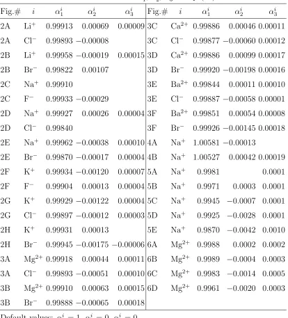
R_iBorn(C_iB) =θ(C_iB)R0_i, θ(C_iB) =α₁i +αi₂CB_i1/2+α₃i CB_i 3/2, (24)

where CB_i = CB

i /M is a dimensionless bulk concentration of type i ions, M is the molar

concentration unit, and αi

1, αi2, and α3i are adjustable parameters for modifying the experi-mental Born radius R0

i to fit experimental activity coefficientsγi that change with the bulk

concentration conditions CB

i of the ion. The Born radii R0i in Table 1 are cited from [25],

which are computed from the experimental hydration Helmholtz free energies of these ions

given in [6]. Numerical values in Tables 1 and 2 are all experimental data for which their

The three parameters in Eq. (24) have physical or mathematical meanings unlike many

parameters in the Pitzer model [41]. Any model or numerical method incurs errors to

approximate a real system, i.e., it is impossible to obtain real Born radiusRBorn

i (CiB) exactly.

The first parameter αi

1 is an adjustment of the experimental Born radiusR0i when CiB = 0

for alli. The second parameter αi

2 is an adjustment of RBorni (CiB) that accounts for the real

thickness of the ionic atmosphere (Debye length), which is proportional to the square root of

the ionic strength√I in the Debye-H¨uckel theory [5]. The third parameter αi

3 is simply an adjustment in the next order approximation beyond the DH treatment of ionic atmosphere.

We summarize the mathematical solution process for determining the activity of ionic

solutions in the following algorithm.

1. Solve Eqs. (9), (10), and (16) forφewith ρ′

= Ψ = 0 (in pure water), RBorn i =R0i,

and φL_=q

i/(4πǫiR0i) to obtain ∆G0i by Eq. (13) and then set φ0e =φe.

2. Solve Eqs. (15) and (17) for Ψ withRBorn

i in (24).

3. Solve Eqs. (9), (10), and (16) forφem with φL=qi/(4πǫiRBorni ) and then set φem−₁ =φe_m.

Go to 2 until convergence.

4. Obtain the activity coefficient γi by Eq. (13).

Table 1. Values of Model Notations

Symbol Meaning Value Unit

kB Boltzmann constant 1.38×10−23 J/K

T temperature Table 2 K

e proton charge 1.602_×10−₁₉

C

ǫ0 permittivity of vacuum 8.85_×10−14

F/cm

ǫion, ǫw dielectric constants 1, Table 2

lc = 2aj correlation length j = Cl

−

etc. ˚A

Ow

i in Eq. (22) 18 [43, 44]

a_Li+, a

Na+, a

K+ radii 0.6, 0.95, 1.33 ˚A

a_Mg2+, a

Ca2+,a

Ba2+ radii 0.65, 0.99, 1.35 ˚A

aF−,a_Cl−, aBr−,aH2O radii 1.36, 1.81, 1.95, 1.4 ˚A

R0

Li+, R0_Na+, R_K0+ Born radii in Eq. (24) 1.3, 1.618, 1.95 ˚A

R0

Mg2+, R0

Ca2+, R0

Ba2+ Born radii 1.424, 1.708, 2.03 ˚A

R0 Cl−, R

0 Cl−, R

0

−0.6 −0.3 0 0.3 0.6

Pos+ by PF Neg− by PF Pos+ by Exp Neg− by Exp

ln γ i (A) Li+ Cl− (B) Li+ Br− −0.6 −0.4 −0.2 0 (C) Na+ F− ln γ i (D) Na+ Cl− (E) Na+ Br−

0 0.5 1 1.5 −0.8 −0.6 −0.4 −0.2 0 (F) K+ F− ln γ i ([PosNeg]/M)1/2

0 0.5 1 1.5 (G)

K+ Cl−

([PosNeg]/M)1/2

0 0.5 1 1.5 (H)

Br− K+

([PosNeg]/M)1/2

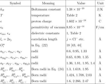
FIG. 2: Indivivual activity coefficients of 1:1 electrolytes. Comparison of PF results with

experi-mental data [26] oni= Pos+_{(cation) and Neg}−

(anion) activity coefficientsγi in various [PosNeg]

from 0 to 1.6 M.

Table 2. Values of ǫw at variousT [51].

T/K 298.15 373.15 423.15 473.15 523.15 573.15

ǫw 78.41 55.51 44.04 38.23 32.23 25.07

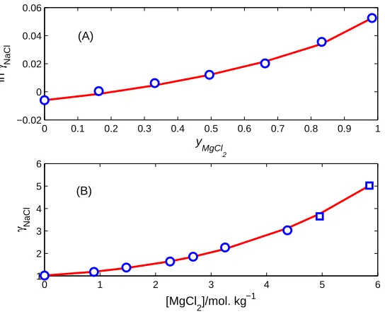
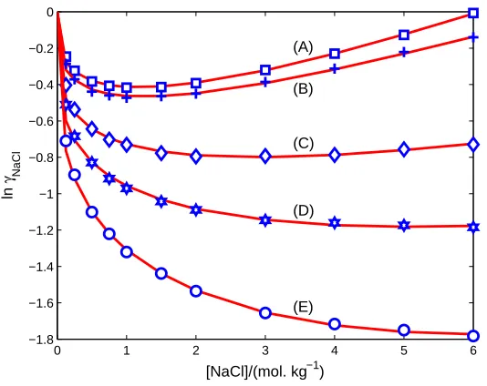
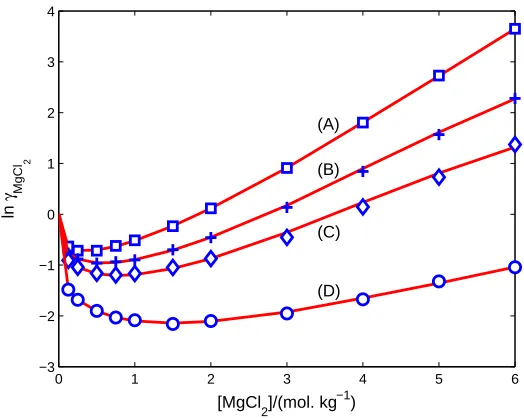
4. RESULTS

The PF results of ionic activity coefficients for eight 1:1 electrolytes, six 2:1 electrolytes,

one mixed electrolyte, one 1:1 electrolyte at various temperatures, and one 2:1 electrolyte

at various temperatures agree with the experimental data [26–35] as shown in Figs. 2, 3, 4,

5, and 6, respectively. The empirical parameters used to fit the experimental data are αi

1, αi

2, and α3i in Eq. (24), whose values are given in Table 3 from which we observe that the PF model requires only one to three parameters to fit those data.

The mean activity coefficient γP osN eg of a salt PospNegq is calculated via the formula

lnγP osN eg = _p+p_qlnγP os+ _p+q_qlnγN eg [5], where γP os and γN eg are individual activity

coeffi-cients obtained by Eq. (13) for each i =P os and Neg. For the mean activity coefficients

−1 0 1

(A)

Pos2+ by PF Neg− by PF

Mg2+

Cl−

ln

γ i

(B)

Mg2+

Br−

−1 0 1

(C)

Pos2+ by Exp Neg− by Exp Ca2+

Cl−

ln

γ i

(D)

Ca2+

Br−

0 0.5 1 1.5 −1.5

−1 −0.5 0

(E)

Ba2+ Cl−

([PosNeg₂]/M)1/2

ln

γ i

0 0.5 1 1.5 (F)

Ba2+ Br−

([PosNeg₂]/M)1/2

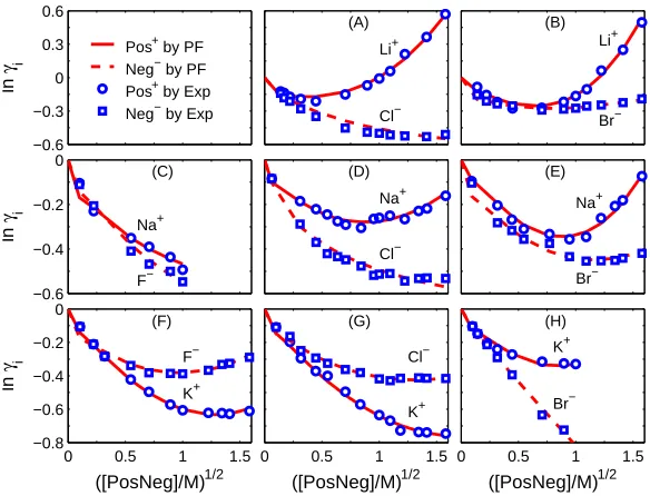
FIG. 3: Indivivual activity coefficients of 2:1 electrolytes. Comparison of PF results with

experi-mental data [26] oni= Pos2+_{(cation) and Neg}−

(anion) activity coefficientsγiin various [PosNeg2]

from 0 to 1.5 M.

parameters of one cation (not all ions) as shown in Table 3.

The activity coefficients by the PF model are quite successful over a large range of

tem-peratures and concentrations as shown in Figs. 4-6. We used the code of the density model

developed by Mao and Duan [52] to convert the concentration unit from molality (mol.

kg−₁

) to molarity (M = mol. dm−₃

) by the standard formula as given in [52], where the

density model has been compared with thousands of measurements at high accuracy. The

pressure values needed in the code at the corresponding temperatures were set to P = (A)

1.01 (B) 1.01 (C) 15.48 (D) 39.59 (E) 80.50 bar for Fig. 4 and (A) 1.01 (B) 1.01 (C) 4.73

(D) 39.50 bar for Fig. 5. In Fig. 6, the ionic strength I =P_iCB

i z2i and the ionic strength

fractionyMgCl2 = 3mMgCl2/(3mMgCl2+mNaCl) with mMgCl2 and mNaClbeing the molalities of

MgCl2 and NaCl in the mixture, respectively, where zi is the valence of type i ions.

We observe from Table 3 that the approximate RBorn

i (CiB) (with salts) deviates from R0i

(without salts) only in the second to fourth decimal place, i.e., numerical values of γi are

very sensitive to the decimal order ofαi

1, αi2, and αi3 because the Born radius RiBorn(CiB) is

very close to the origin 0 at which the singular charge inρi(r) =qiδ(r−0) is infinite. The

approximation of the shell radiusRSh

i (or the coordination number Oiw in Eq. (22)), on the

other hand, is much less significant than that ofRBorn

0 0.1 0.2 0.3 0.4 0.5 0.6 0.7 0.8 0.9 1 −0.02

0 0.02 0.04 0.06

(A)

y

MgCl

2

ln

γ NaCl

0 1 2 3 4 5 6

1 2 3 4 5 6

(B)

[MgCl₂]/mol. kg−1

γ NaCl

FIG. 4: Mean activity coefficients of mixed electrolytes. Comparison of PF results (curve) with

experimental data (symbols) compiled in [13] (A) from [33] on mean activity coefficientsγ of NaCl

as a function of the ionic strength (I) fractionyMgCl2of MgCl2 in NaCl + MgCl2 mixtures atI = 6

mol. kg−₁

and T = 298.15 K; (B) from [34] (circles) and [35] (squares) onγ of NaCl as a function

of the MgCl2 molality in NaCl + MgCl2 mixtures at [NaCl] = 6 mol. kg−1 and T = 298.15 K.

diminishes exponentially in the hydration shell region Ωsh as shown by the profile ofφPF(r)

in Fig. 7. The values of αi

1, αi2, and α3i for each activity-concentration curve were obtained by first tuning three values of θ(CB

i ) in Eq. (24) to match three data points ( q

CB

ij, lnγij)

with three different concentrations CB

ij, j = 1, 2, 3, and then solving the three unknowns

αi

1, αi2, and αi3 using three known θ(CijB) values. For example, for the i = Li+ curve in Fig.

2A, the selected experimental data points are (qCB

ij, lnγij) = (0.315, -0.192), (1, -0.007),

(1.577, 0.57) and the corresponding tuned θ(CB

ij) are 0.9996, 1.0013, 1.0043.

The PF model can provide more physical details near the solvated ion (Ca2+_{, for example)}

in a strong electrolyte ([CaCl2] = 2 M) such as (1) the dielectric functioneǫ(r) with its varying

permittivity, (2) variable water densityCH2O(r), (3) concentration of counterionCCl−(r), (4)

electric potential φPF_{(r), and (5) the steric potential S}trc_{(r) all shown in Fig. 7. The steric}

potential is small because the configuration of particles (voids between particles) does not

vary too much from the solvated region to the bulk region. Nevertheless, it has significant

0 1 2 3 4 5 6 −1.8

−1.6 −1.4 −1.2 −1 −0.8 −0.6 −0.4 −0.2 0

(A)

(B)

(C)

(D)

(E)

[NaCl]/(mol. kg−1)

ln

γ NaCl

FIG. 5: Mean activity coefficients of 1:1 electrolyte at various temperatures. Comparison of PF

results (curves) with experimental data (symbols) compiled in [13] from [27–29] on mean activity

coefficients γ of NaCl in [NaCl] from 0 to 6 mol. kg−1

at T = (A) 298.15 (B) 373.15 (C) 473.15

(D) 523.15 (E) 573.15 K.

function _eǫ(r) in the hydration region. Note that _eǫ(r) is an output, not an input of the

model.

The strong electric potentialφPF_{(r) in the Born cavity Ω}

i (withRBorni (CiB) = 1.7130 ˚A)

and the water density CH2O(r) in the hydration shell Ωsh (with R sh

Ca2+ = 5.0769 ˚A) are the

most important factors allowing the PF results to match the experimental data. The ion and

shell domains are the crucial region to study ion activities. For example, Fraenkel’s theory is

entirely based on this region — the so-called smaller-ion shell region [41]. The steric energy

of water molecules modified by the factor vK+1/v0 in Eq. (5) leads to significant changes of

CH2O(r) and eǫ(r) profiles in Fig. 7 as compared with those in Fig. 5 in our previous paper

0 1 2 3 4 5 6 −3

−2 −1 0 1 2 3 4

(A)

(B)

(C)

(D)

[MgCl

2]/(mol. kg −1

)

ln

γ MgCl

2

FIG. 6: Mean activity coefficients of 2:1 electrolyte at various temperatures. Comparison of PF

results (curves) with experimental data (symbols) compiled in [13] from [30–32] on mean activity

coefficients γ of MgCl2 in [MgCl2] from 0 to 6 mol. kg−1 at T = (A) 298.15 (B) 373.15 (C) 423.15

Table 3. Values of αi

1, αi2, αi3 in Eq. (24) Fig.# i αi

1 α2i αi3 Fig.# i αi1 α2i αi3 2A Li+ _{0.99913 0.00069 0.00009 3C Ca}2+ _{0.99886 0.00046 0.00011}

2A Cl−

0.99893 ₋0.00008 3C Cl−

0.99877 ₋0.00060 0.00012

2B Li+ _{0.99958 −0.00019 0.00015 3D Ca}2+ _{0.99886 0.00099 0.00017}

2B Br−

0.99822 0.00107 3D Br−

0.99920 ₋0.00198 0.00016

2C Na+ _{0.99910 3E Ba}2+ _{0.99844 0.00011 0.00010}

2C F−

0.99933 ₋0.00029 3E Cl−

0.99887 ₋0.00058 0.00001

2D Na+ _{0.99927 0.00026 0.00004 3F Ba}2+ _{0.99851 0.00054 0.00008}

2D Cl−

0.99840 3F Br−

0.99926 ₋0.00145 0.00018

2E Na+ _{0.99962 −0.00038 0.00010 4A Na}+ _{1.00581 −0.00013}

2E Br−

0.99870 ₋0.00017 0.00004 4B Na+ _{1.00527 0.00042 0.00019}

2F K+ _{0.99934 −0.00120 0.00007 5A Na}+ _{0.9981 0.0001}

2F F−

0.99904 0.00013 0.00004 5B Na+ _{0.9971 0.0003 0.0001}

2G K+ _{0.99929 −0.00122 0.00004 5C Na}+ _{0.9945 −0.0007 0.0001}

2G Cl−

0.99897 ₋0.00012 0.00003 5D Na+ _{0.9925 −0.0028 0.0001}

2H K+ _{0.99931 0.00013 5E Na}+ _{0.9870 −0.0042 0.0010}

2H Br−

0.99945 ₋0.00175 ₋0.00006 6A Mg2+ _{0.9988 0.0002 0.0002}

3A Mg2+ _{0.99918 0.00044 0.00011 6B Mg}2+ _{0.9989 −0.0004 0.0003}

3A Cl−

0.99893 ₋0.00051 0.00010 6C Mg2+ _{0.9983 −0.0014 0.0005}

3B Mg2+ _{0.99910 0.00063 0.00015 6D Mg}2+ _{0.9961 −0.0020 0.0003}

3B Br−

0.99888 ₋0.00065 0.00018

Default values: αi

1 = 1, αi2 = 0, α3i = 0.

5. CONCLUSION

A Poisson-Fermi model for calculating activity coefficients of aqueous single or mixed

electrolyte solutions in a large range of concentrations and temperatures has been presented

and tested by a set of experimental data. The model was shown to well fit experimental

data with only three adjustable parameters at most for each activity-concentration curve.

The adjustable parameters correspond to different orders of approximation of the unknown

0 5 10 15 20 50

55 60 65 70 75 80 85 90

r

ε

,

C H2O

0 5 10 15 20

−2 0 2 4 6 8 10 12

r

[Cl

− ],

φ

,

S

trc

ε C

H2O in M

[Cl−] in M

φ in k

BT/e

Strc in k

BT

FIG. 7: Dielectric function_eǫ(r) (denoted by εin the figure), water density CH2O(r) (CH2O), Cl

−

concentration C_Cl−(r) ([Cl

−

]), electric potential φPF(r) (φ), and steric potential Strc(r) (Strc)

profiles near the solvated ion Ca2+ at [CaCl2] = 2 M, where r is the distance from the center of

Ca2+ in Angstrom.

and nonlinear way. Nevertheless, the values of these parameters have been shown to deviate

slightly in decimal digits from that of the experimental Born radius in pure water. These

parameters are physically explained and can be easily verified in future studies for the same

or different solutions of the present work. The model requires very few parameters because

it is based on an advanced continuum theory that accounts for steric and correlation effects

of ions and water with interstitial voids between nonuniform hard spheres. It also deals with

short- and long-range interactions by partitioning the model domain into the ion, hydration

shell, and the remaining solvent sub-domains. Numerical methods were also given to show

how to solve different equations on different sub-domains that describe different physical

Acknowledgments

This work was supported by the Ministry of Science and Technology, Taiwan (MOST

105-2115-M-007-016-MY2 to J.L.L.).

[1] R. Robinson and R. Stokes, Electrolyte Solutions (Butterworths Scientific Publications, Lon-don, 1959); (Dover Publications, New York, 2002).

[2] J. Newman,Electrochemical Systems (Prentice-Hall, NJ, 1991). [3] K. S. Pitzer,Thermodynamics (McGraw Hill, New York, 1995).

[4] B. Hille, Ionic Channels of Excitable Membranes (Sinauer Associates Inc., Sunderland, MA, 2001).

[5] K. J. Laidler, J. H. Meiser, and B. C. Sanctuary, Physical Chemistry (Houghton Mifflin Co., Boston, 2003).

[6] W. R. Fawcett, Liquids, Solutions, and Interfaces: From Classical Macroscopic Descriptions to Modern Microscopic Details (Oxford University Press, New York, 2004).

[7] G. Lebon, D. Jou, and J. Casas-V´azquez, Understanding Non-equilibrium Thermodynamics: Foundations, Applications, Frontiers (Springer, 2008).

[8] G. M. Kontogeorgis and G. K. Folas, Thermodynamic Models for Industrial Applications: From Classical and Advanced Mixing Rules to Association Theories (John Wiley & Sons, 2009).

[9] W. Kunz,Specific Ion Effects (World Scientific, Singapore 2010).

[10] J. H. Vera and G. Wilczek-Vera, Classical Thermodynamics of Fluid Systems: Principles and

Applications (CRC Press, 2016).

[11] W. Voigt, Chemistry of salts in aqueous solutions: Applications, experiments, and theory.

Pure Appl. Chem. 83, (2011) 1015-1030.

[12] B. Eisenberg, Interacting ions in Biophysics: Real is not ideal, Biophys. J. 104, 1849-1866

(2013).

[13] D. Rowland, E. K¨onigsberger, G. Hefter, and P. M. May, Aqueous electrolyte solution

mod-elling: Some limitations of the Pitzer equations, Appl. Geochem. 55, 170 (2015).

ver-wandte Erscheinunge (The theory of electrolytes. I. Lowering of freezing point and related

phenomena), Phys. Zeitschr. 24, 185-206 (1923).

[15] M. Gouy, Sur la constitution de la charge electrique a la surface d’un electrolyte (Constitution

of the electric charge at the surface of an electrolyte), J. Phys. 9 (1910) 457-468.

[16] D. L. Chapman, A contribution to the theory of electrocapillarity, Phil. Mag. 25, 475-481

(1913).

[17] J.-L. Liu, Numerical methods for the Poisson-Fermi equation in electrolytes, J. Comput. Phys.

247, 88 (2013).

[18] J.-L. Liu, D. Xie, and B. Eisenberg, Poisson-Fermi formulation of nonlocal electrostatics in

electrolyte solutions, Mol. Based Math. Biol. 5, 116-124 (2017).

[19] J.-L. Liu and B. Eisenberg, Poisson-Fermi model of single ion activities in aqueous solutions,

Chem. Phys. Lett. 637, 1-6 (2015).

[20] J.-L. Liu and B. Eisenberg, Correlated ions in a calcium channel model: a Poisson-Fermi

theory, J. Phys. Chem. B 117, 12051 (2013).

[21] J.-L. Liu and B. Eisenberg, Poisson-Nernst-Planck-Fermi theory for modeling biological ion

channels, J. Chem. Phys. 141, 22D532 (2014).

[22] J.-L. Liu and B. Eisenberg, Analytical models of calcium binding in a calcium channel, J.

Chem. Phys. 141, 075102 (2014).

[23] J.-L. Liu and B. Eisenberg, Numerical methods for a Poisson-Nernst-Planck-Fermi model of

biological ion channels, Phys. Rev. E92, 012711 (2015).

[24] J.-L. Liu, H.-j. Hsieh, and B. Eisenberg, Poisson-Fermi modeling of the ion exchange

mecha-nism of the sodium/calcium exchanger, J. Phys. Chem. B 120, 2658-2669 (2016).

[25] M. Valisk´o, D. Boda, Unraveling the behavior of the individual ionic activity coefficients on

the basis of the balance of ion-ion and ion-water interactions, J. Phys. Chem. B 119, 1546

(2015).

[26] G. Wilczek-Vera, E. Rodil, and J. H. Vera, On the activity of ions and the junction potential:

Revised values for all data, AIChE. J. 50, 445 (2004).

[27] K. S. Pitzer, J. C. Peiper, and R. H. Busey, Thermodynamic properties of aqueous sodium

chloride solutions, J. Phys. Chem. Ref. Data 13, 1-102 (1984).

[28] R. H. Busey, H. F. Holmes, and R. E. Mesmer, The enthalpy of dilution of aqueous sodium

thermody-namic properties and their pressure coefficients, J. Chem. Thermodyn. 16, 343-372 (1984).

[29] D. G. Archer, Thermodynamic properties of the NaCl + H2O System. II. Thermodynamic

properties of NaCl(aq), NaCl.2H2O(cr), and phase equilibria, J. Phys. Chem. Ref. Data 21,

793-829 (1992).

[30] R. N. Goldberg and R. L. Nuttall, Evaluated activity and osmotic coefficients for aqueous

solutions: The alkaline earth metal halides, J. Phys. Chem. Ref. Data 7, 263-310 (1978).

[31] P. Wang, K. S. Pitzer, and J. M. Simonson, Thermodynamic properties of aqueous magnesium

chloride solutions from 250 to 600 K and to 100 MPa, J. Phys. Chem. Ref. Data 27, 971-991

(1998).

[32] C. Christov, Chemical equilibrium model of solution behavior and bishofite (MgCl_2·6H2O(cr))

and hydrogen-carnallite (HCl_·MgCl2·7H2O(cr)) solubility in the MgCl2+ H2O and HCl-MgCl2

+ H2O systems to high acid concentration at (0 to 100)◦C, J. Chem. Eng. Data54, 2599-2608

(2009).

[33] R. D. Lanier, Activity coefficients of sodium chloride in aqueous three-component solutions

by cation-sensitive glass electrodes, J. Phys. Chem. 69, 3992-3998 (1965).

[34] N. Kurnakov and S. F. Zemcuzny, Equilibria in the reciprocal system sodium

chloride-magnesium sulfate with particular reference to natural brines, Z. Anorg. Allg. Chem. 140,

149-182 (1924).

[35] S. Takegami, Reciprocal salt pairs: Na2Cl2+ MgSO4 and Na2SO4+ MgCl2at 25◦C, Memoirs

College Sci. Kyoto Imperial Univ. 4, 317-342 (1921).

[36] G. Wilczek-Vera and J. H. Vera, On the measurement of individual ion activities, Fluid Phase

Equilibria 236, 96-110 (2005).

[37] G. Wilczek-Vera, E. Rodil, and J. H. Vera, A complete discussion of the rationale supporting

the experimental determination of individual ionic activities, Fluid Phase Equilibria 244,

33-45 (2006).

[38] G. Wilczek-Vera and J. H. Vera, Peculiarities of the thermodynamics of electrolyte solutions:

A critical discussion, Can. J. Chem. Eng. 81, 70-79 (2003).

[39] G. Wilczek-Vera and J. H. Vera, The activity of individual ions. A conceptual discussion of the

relation between the theory and the experimentally measured values, Fluid Phase Equilibria

312, 79-84 (2011).

J. Chem. Thermodynamics 9, 65-69 (2016).

[41] D. Fraenkel, Simplified electrostatic model for the thermodynamic excess potentials of binary

strong electrolyte solutions with size-dissimilar ions, Mol. Phys. 108, 1435 (2010).

[42] D. Bashford and D. A. Case, Generalized Born models of macromolecular solvation effects,

Annu. Rev. Phys. Chem. 51, 129 (2000).

[43] W. W. Rudolph and G. Irmer, Hydration of the calcium(II) ion in an aqueous solution of

common anions (ClO− 4, Cl

−

, Br−

, and NO−

3), Dalton Trans.42, 3919 (2013).

[44] J. M¨ahler and I. Persson, A study of the hydration of the alkali metal ions in aqueous solution,

Inorg. Chem. 51, 425 (2011).

[45] B. Eisenberg, Life’s solutions: a mathematical challenge, arXiv:1207.4737 (2012).

[46] C. D. Santangelo, Computing counterion densities at intermediate coupling, Phys. Rev. E73,

041512 (2006).

[47] M. Z. Bazant, B. D. Storey, and A. A. Kornyshev, Double layer in ionic liquids: Overscreening

versus crowding, Phys. Rev. Lett. 106, 046102 (2011).

[48] I-L. Chern, J.-G. Liu, and W.-C. Wang, Accurate evaluation of electrostatics for

macro-molecules in solution, Methods Appl. Anal. 10, 309-328 (2003).

[49] W. Geng, S. Yu, and G. Wei, Treatment of charge singularities in implicit solvent models, J.

Chem. Phys. 127, 114106 (2007).

[50] R. S. Dembo, S. C. Eisenstat, and T. Steihaug, Inexact Newton methods, SIAM J. Numer.

Anal.19, 400-408 (1982).

[51] D. P. Fernandez, A. R. H. Goodwin, E. W. Lemmon, J. L. Sengers, and R. C. Williams, A

formulation for the static permittivity of water and steam at temperatures from 238 K to 873

K at pressures up to 1200 MPa, including derivatives and Debye–H¨uckel coefficients, J. Phys.

Chem. Ref. Data 26, 1125-1166 (1997).

[52] S. Mao and Z. Duan, TheP, V, T, x properties of binary aqueous chloride solutions up to T =