Global optimization of mixed-integer polynomial programming problems: A new method based on Grobner Bases theory

Author name / Procedia CIRP 00 (2011) 000–001

Global optimization of mixed-integer polynomial programming

problems: A new method based on Grobner bases theory

Ali Papi

_{, Armin Jabbarzadeh}

_{, Adel Aazami}

papimath@hotmail.com, arminj@iust.ac.ir, adel.aazami@yahoo.com

Abstract

Mixed-integer polynomial programming (MIPP) problems are one class of mixed-integer nonlinear programming (MINLP) problems where objective function and constraints are restricted to the polynomial functions. Although the MINLP problem is NP-hard, in special cases such as MIPP problems, an efficient algorithm can be extended to solve it. In this research, we propose an algorithm for global optimization of the MIPP problems, in which, first, the MIPP is reformulated as a multi-parametric programming by considering integer variables as parameters. Then, the optimality conditions of resulting parametric programming give a parametric polynomial equations system (PES) that is solved analytically by Grobner Bases (GB) theory. After solving PES, the parametric optimal solution as a function of the relaxed integer variables is obtained. A simple discrete optimization problem is resulted for any non-imaginary parametric solution of PES, which the global optimum solution of MIPP is determined by comparing their optimal value. Some numerical examples are provided to clarify proposed algorithm and extend it for solving the MINLP problems. Finally, a performance analysis is conducted to demonstrate the practical efficiency of the proposed method.

Keywords:

1-Introduction

The mixed integer non-linear programming (MINLP) problem is a class of optimization problems with both continuous and integer variables where the objective function or some of the constraints are not linear. Many decision problems such as scheduling (Cafaro et al.,2015), distribution systems (Kaur et al.,2014), water networks (Tokos et al.,2013), layout design (de Lira-Flores et al.,2014) supply chains under stochastic demand (Li and Yu,2016), construction structures (Kravanja et al.,2013), chemical processes (Kraemer et al.,2007), etc., can be modelled as MINLP. In general, these problems are modelled as (1) where x is the vector of continuous variables and y is the vector of integer variables. *Corresponding author

ISSN: 1735-8272, Copyright c 2018 JISE. All rights reserved

Journal of Industrial and Systems Engineering

Vol. 11, Special issue: 14th International Industrial Engineering Conference

Summer (July) 2018, pp. 1-15

(IIEC 2018)

TEHRAN, IRAN

1

In order to achieve a general finite optimum, the proposed algorithms generally assumed that the objective function (f) and all constraint functions (fi ,gi) are convex. Vectors x and y belong to compact and convex subsets in _X ⊂_Rnx _{and Y} ⊂_Znx _{, respectively, and f is defined on the Cartesian (X×Y).}

(1)

( , ) . .

( , ) 0 1, 2, 3,..., ( , ) 0 1, 2, 3,...,

i h

i g

Min z f x y s t

h x y i n

g x y i n

= 

 

 _{= =}



 ≤ =



However, the stated assumptions do not change the difficulty of MINLP problems and these are still NP-hard. Although many studies have been done to solve MINLP problems and different solving approaches have been introduced, the algorithm with polynomial computational complexity is not yet known to be capable of solving them. In general, these approaches can be divided into two categories: deterministic and stochastic. Most of deterministic algorithms for MINLP problems that guarantee global optimal solution (as detailed or sometimes approximate) are convex. Convexity and compactness of the solution space and objective function ensures that the obtained solution is global optimum. Branch and bound methods (Gupta and Ravindran,1985), (Kirst et al.,2016), (Quesada and Grossmann,1992) extended cutting plane method (Westerlund and Pettersson,1995) and outer approximation (OA) method (Duran and Grossmann,1986), (Fletcher and Leyffer,1994) are examples of the deterministic methods to solve the convex MINLP problems. In these approaches, the first condition of the integer y is usually ignored and then, by defining the problem or providing some methods such as the branch and bound, the optimal solution is determined which satisfies the integer condition. A good example for the convex problems is the next investigated research. In (Gu et al., 2016), an optimization problem is considered that minimizes a function of the form 𝑓𝑓 =𝑓𝑓₀+𝑓𝑓₁−

𝑓𝑓2with the constraint𝑔𝑔 − ℎ ≤0, where 𝑓𝑓0is continuous differentiable, 𝑓𝑓1,𝑓𝑓2 are convex and 𝑔𝑔,ℎ are

lower semi-continuous convex. Other non-deterministic algorithms (random search) for solving MINLP problems are usually based on some properties of nature. These algorithms can also be divided into two categories: meta-heuristic and heuristic algorithms; meta-heuristic algorithms such as genetics (Deep et al., 2009), Tabu search (Lin et al., 2003), simulated annealing (Cardoso et al., 1997), etc., are adaptable to various problems, while heuristic algorithms are used to solve specific problems more efficiently and they are sometimes used to improve meta-heuristic algorithms (Bertacco et al., 2007).

The mentioned algorithms can be implemented mainly on convex problems, and using these approaches in non-convex problems allows stopping at the local optimal solution rather than the global optimal solution. Therefore, various studies have also been carried out in this field, and some approaches are presented for solving non-convex MINLP problems, such as maximum cutting method (Anjos and Vannelli, 2008), (Goemans and Williamson, 1995), clustering (Sherali and Desai, 2005) and optimization of polynomials (Lasserre, 2001). In addition, some researchers have presented a solution for non-convex MINLP problems through using the existing signomial (generalized geometric) expressions. In most cases, non-convex MINLP problems are at least as hard as their convex counterparts are considered as NP-hard.

In recent years, many studies have been conducted to find the global optimal solution of MINLP problems and various methods are suggested, such as LCA algorithms, results of which show the performance and stability of these algorithms (Yan et al., 2004). In Eronen et al.,( 2017), the extended hyperplane algorithm is generalized for a convex continuously differentiable MINLP problem to solve a class of non-smooth problems. A number of studies have also been conducted on the improvement of the efficiency of previous algorithms, among which strategies to improve the efficiency and convergence of computing OA algorithms and analysis Benders could be noted (Su et al., 2015). It should be noted that, efficiency here means that by increasing the problem dimension, the time taken to find the optimal solution would have less growth and deviation of the presented solution would be lower than that of the global optimal value.

Recently, some more efficient methods are proposed for a variety of the NLP models, among which (Crama and Rodríguez-Heck, 2017) and (Kim and Kojima, 2017) can be mentioned. In Crama and

Rodríguez-Heck ( 2017) , a new class of valid inequalities for binary optimization problems is proposed to strengthen the LP relaxation of the standard linearization. In Kim and Kojima (2017), conic relaxations containing doubly nonnegative programming (DNN) relaxations and semi definite programming (SDP) relaxations are investigated to earn the optimal values of binary quadratic problems.

Although none of algorithms proposed to solve the MINLP problems generally can be given preference over another, it can be claimed that for special problems, some algorithms are more efficient than others are. Therefore, the MINLP problems could be classified into different categories, and various approaches could be provided to have greater performance in each class. A specific class of MINLP problems is mixed-integer polynomial programming (MIPP), where the objective function and constraints are limited to polynomials. MIPP problems can be evaluated specifically and solved by developing efficiency approaches. Based on Karush–Kuhn–Tucker (KKT) conditions, the optimal solution of an optimization problem is obtained by solving the system of equations. In some cases where the objective function or constraints are not linear, the system of equations becomes non-linear and generally, it is not possible to solve them analytically and accurately. While if the non-linearity of the problem is limited to polynomials, the result is a system of polynomial equations that can be solved based on Grobner Bases (GB) theory (Buchberger, 2001). Some research have been previously done, which used the GB theory to solve continuous polynomial optimization problems (Chang et al., 1994) and (Hägglöf et al., 1995). In this paper, a new method based on the GB theory is proposed for solving MIPP problems. Although these problems are not necessarily convex, the proposed method can determine the global optimal solution of these problems. In addition, some MINLP problems are convertible to the MILP by using the Taylor series, and their optimal solution can be approximated with desired accuracy by using this method.

The remaining sections are organized as follows. In Section 2, the general form of MIPP and parametric polynomial programming (PPP) problems are presented. In Section 3, a methodology is proposed for solving the MIPP problem with complete details. Section 4 presents the proposed method for solving the MIPP problem as a step-by-step algorithm. In Section 5, three various numerical examples are presented to further explain how to use the proposed method. In Section 6, in order to investigate the practical efficiency of the proposed algorithm, a performance analysis is done. In Final Section, the conclusion and some suggestions for further studies are presented.

2-Mixed-Integer Polynomial Programming (MIPP) and Parametric Polynomial

Programming (PPP)

If in the generic form of MINLP, the objective function and constraints are polynomials function according to the variable vectors x and y, MIPP problems are obtained. Here, the variables in the compact space are defined as the model (2).

(2)

( , ) . .

( , ) 0 1, 2, 3,..., ( , ) 0 1, 2, 3,...,

1, 2, 3,...,

{ , 1,..., } 1, 2, 3,...,

, .

i h

i g

xk k xk x

k yk yk yk y

i i

Min f x y s t

h x y i n

g x y i n

L x U k n

y L L U Integert numbers k n

f g and h are polynomial function respect to x and y

  

 _{= =}



 _{≤ =}



 _{≤ ≤ =}



 _{∈ + ⊂ =}

 

In optimization problems, if at least one of the numerical values of the parameters in the model does not exist, then the optimal solution is calculated based on this parameter and for each value of it, the corresponding optimal solution is obtained; these types of problems are presented as parametric programming problems. Assume that in the model (2), vector y is one of the parameters of the problem and vector x is the only variable of the problem. In this case, the model (2) is reformulated as a polynomial parametric programming problem (model (3)), in which the optimal solution is obtained based on y.

(3)

( )

( ) ( )

( ) . .

( ) 0 1, 2, 3,..., ( ) 0 1, 2, 3,...,

y y

y

i h

y

i g

Min Z f x

s t

h x i n

g x i n

 =

  

= =



 _{≤ =}



3-Methodology

In order to solve the given MIPP problem (the model (2)), the following three-step methodology is proposed:

Step 1: solve the model (3) as a parametric model to obtain the optimal candidate solution based on y. Call each of these solutions s_{x y|} .

Step 2: for each solutionsx y| , formulate an integer optimization problem that its objective function is

based on y as ( ) ( | ) y

s x y

F y =f s . Vector y changes in the allowed domain

1

{ , 1,..., }

y

n

yk yk yk k

L L U

=

+

∏

each of these problemsP s( _{x y|} ).

Step 3: determine the optimal solution by comparing the optimal and feasible values of each problem

|

( _{x y}) P s .

The following sections describe how to do the above steps in details.

3-1-Solving the parametric model and finding optimal candidate solution

The optimal solution of a mathematical programming problem is applied to a system of equations (and sometimes inequalitiesa_{) which is made from the corresponding KKT conditions. In other words,}

a necessary condition for optimality of each answer is that it satisfies the KKT conditions. Consider the following mathematical programming problem:

(4)

1 2

( ) . .

( ) 0 1, 2, 3,...,

; ( , ,..., ) ( ) 0 1, 2, 3,...,

i H

n

i G

Min F X s t

H X i n

X x x x

G X i n

 

 _{= =}



 ₌



 ≤ =



Lagrange function corresponding to the above model is defined as (X,λ,μ) = F(X) +

∑nH λ_i

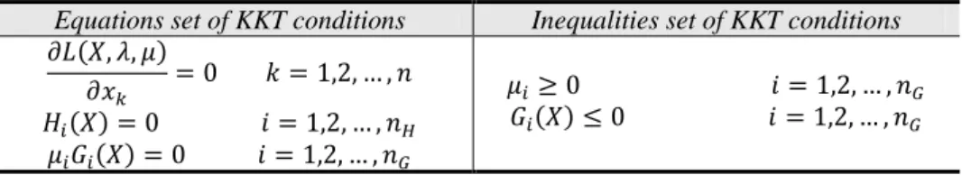
i=1 Hi(X) +∑ni=1G μiGi(X). By applying the KKT conditions, systems of equations and inequalities

related to this problem are formulated, as seen in table 1.

Table 1. Systems of equations and inequalities of the KKT conditions

Inequalities set of KKT conditions Equations set of KKT conditions

𝜇𝜇𝑖𝑖≥0 𝑖𝑖= 1,2, … ,𝑛𝑛𝐺𝐺 𝐺𝐺𝑖𝑖(𝑋𝑋)≤0 𝑖𝑖= 1,2, … ,𝑛𝑛𝐺𝐺 𝜕𝜕𝜕𝜕(𝑋𝑋,𝜆𝜆,𝜇𝜇)

𝜕𝜕𝑥𝑥𝑘𝑘 = 0 𝑘𝑘= 1,2, … ,𝑛𝑛 𝐻𝐻𝑖𝑖(𝑋𝑋) = 0 𝑖𝑖= 1,2, … ,𝑛𝑛𝐻𝐻 𝜇𝜇𝑖𝑖𝐺𝐺𝑖𝑖(𝑋𝑋) = 0 𝑖𝑖= 1,2, … ,𝑛𝑛𝐺𝐺

To find the optimal candidate solution of the model (4), the system of equations must be solved first and then, each of the obtained solutions that also satisfy inequalities is considered as an optimal candidate solution. In most nonlinear cases, solving a system of equations is not possible and its solutions can be approximated only by using some numerical methods such as Newton-Raphson. Nevertheless, a polynomial equations system (PES) is obtained in MIPP problems, and fortunately,

a _{If there are inequality constraints on the problem, some inequalities also exist in the system.}

4

there are analytical and accurate methods for solving the PES in both numeric and parametric cases. PES solving methods are mainly derived from the GB theory, the most important of which is Buchberger algorithm (Buchberger, 2001) (read more in Boege et al. (1986)). The Buchberger algorithm first obtains the foundations of the initial Grobner PES and then, forms a new PES with its answer as equal to the initial PES answers, which can be solved as a system of linear equations is solved. This algorithm has been provided in MATLAB, MATHEMATICA, and MAPLE.

If in the MIPP problem, we consider the integer variables vector y as parameters, then, according to Table 1, the parametric PES (5) is obtained. By solving the system (5), its solutions are obtained as x(y),λ(y),μ(y). Suppose that Sx y| is a set of all non-imaginary solutions of PES; each of sx y| ∈Sx y| is

an optimal candidate solution.

(5)

(

)

_{( )}

( )

_{( )}

0 ; 1: , 0 ; 1: , 0 ; 1:

y y

x i h

k y

i i g

L x

k n h x i n

x

g x i n

λ µ µ

∂ 

= ∀ = = ∀ =

 _∂ 

 

 _{= ∀ =} 

 

3-2-Feasibility and optimality of optimal candidate solution

For each value in the changes domain of y, each parametric solution sx y| ∈Sx y| converts into a

numerical solution; if this solution satisfies inequalities of the KKT conditions, it is a feasible and optimal candidate, and otherwise, it should be removed. For eachsx y| ∈Sx y| , objective function of the

MIPP problem converts into a function of y as ( ) ( | )

y

s x y

F y =f s ; each feasible and optimal candidate

solution gives a value to the objective function, which is an optimal candidate solution. In other words, to examine eachsx y| ∈Sx y| , integer optimization problem P s( x y| )can be defined where its constraints are

inequalities system related to the KKT conditions and its objective function is reformulation by the parametric solution. By solving the model (6), the optimum value of integer variables will be determined and according tosx y| , the optimum value of continuous variables is calculated. Note that for solving

the model (6), different approaches such as counting, branch and bound and cutting plane methods can be used. Also, in some cases where the number of variables is large, meta-heuristic and heuristic approaches can be applied to integer optimization (Deep et al., 2009) and (Lin et al., 2003) and (Cardoso et al., 1997). However, in this section, providing a new heuristic algorithm can increase the effectiveness of the proposed method.

(6)

|

|

( ) :

( ) ( )

. .

( ) 0 1, 2,3,..., ( ) 0 1, 2,3,...,

{ , 1,..., } 1, 2,...,

x y

y

s x y

i g

i g

k yk yk yk y

P s

Min F y f s

s t

y i n

g y i n

y L L U Integert numbers k n

µ  

= 

 

 _{≥ =}



 _{≤ =}



 ∈ + ⊂ =



3-3-Comparison of the parametric solution and determination of the optimal solution

For each feasibleP s( x y| ), let the optimal value of the objective function be x y| opt s

F and the optimal solution of decision variables be ( x y| , ( x y| ))

opt opt

s s

y x y . Moreover, for unjustified problems, let x y| opt s

F = +∞. To determine the optimal solution of the MIPP problem, these values should be compared and the minimum amount of them has to be determined.

We define |

*

| |

min{ opt_{x y} | }

s x y x y

Z = F s ∈S ; if _Z*_{= +∞, then the problem is infeasible; otherwise, the}

parametric solution that has led to _Z*_{is the global optimum solution, and we will display it by} * | . x y

optimal value of decision variables is obtained bys*x y| and it is equal to * *

| |

* *

( , ) ( , ( ))

x y x y

opt opt

s s

y x = y x y . Note that

* | x y

s may not be unique and sometimes more than one sx y| ∈Sx y| lead to *

Z .

4-The proposed algorithm for solving MIPP

The proposed algorithm for solving this type of problems is described as a step-by-step algorithm in table 2.

Table 2. The proposed algorithm

Step 0 Input the MIPP problem with integer variables y and continuous variables x.

(Minimizing the MIPP problem)

Step 1 Consider the integer variables as parameters and relax the problem to a

parametric polynomial programming (PPP) problem.

Step 2 Formulate Lagrange function corresponding to the PPP problem.

Step 3 Apply the KKT conditions to the PPP problem and determine equations and

inequalities system of the KKT conditions.

Step 4 Formulate the polynomial equations system (PES) from the equations system

of the KKT conditions.

Step 5 Solve the PES based on the GB theory (Using the proposed Mathematica

Software). If PES has no non-imaginary solutions, then the MIPP problem is infeasible andthe procedure stops, Otherwise go to Step 6.

Step 6 Formulate the integer optimization problem corresponding to each

non-imaginary solution of PES, and solve it based on a counting method.

Step 7 Record the optimum value of objective functions for each integer

optimization problem, corresponding to each non-imaginary solution, in set “O”. For each of them that is infeasible, Record + ∞ in the set “O”.

Step 8 Find the minimum value of the set O and name it Z*. If Z* is equal to + ∞,

the MIPP problem is infeasible and the procedure stops; Otherwise go to Step 9.

Step 9 Display Z* and (y*, x*) as the optimal solution.

Note that the above algorithm works quite similar for MINLP problems with the difference at Step 0 where the input MINLP problem is relaxed as the MIPP problem based on the Taylor expansion of functions. In these problems, although the number of long sentences from Taylor expansion functions increases problem-solving time, a better approximation of a global optimum solution is obtained.

5-Numerical examples

In this section, three numerical examples are illustrated to learn how to use the proposed method for solving MIPP problems. Example 1 is an MIPP problem with a binary-integer variable. In Example 2, the integer variables are not necessarily limited to binary numbers. Finally, example 3 shows an MINLP problem that firstly is converted to the MIPP problem and then, is solved by the proposed approach.

5-1-Example 1: The MIPP problem with binary variables

This example is in the form of model (7):

(7)

𝑀𝑀𝑀𝑀𝑥𝑥𝑍𝑍= 10𝑥𝑥12𝑦𝑦1+ 13𝑥𝑥22𝑦𝑦2− 𝑥𝑥3𝑦𝑦3−100𝑦𝑦1−80𝑦𝑦2+ 200𝑦𝑦3

𝑠𝑠.𝑡𝑡.

𝑦𝑦1+𝑦𝑦2+𝑦𝑦3 = 2

𝑥𝑥12+𝑥𝑥22+𝑥𝑥32≤100

−10≤ 𝑥𝑥𝑘𝑘 ≤10 𝑘𝑘= 1,2,3

𝑦𝑦𝑘𝑘 ∊{0,1} 𝑘𝑘= 1,2,3

By relaxing binary variables (y₁, y₂, y₃) as parameters, Lagrange function corresponding to Example 1 is constructed as follows:

𝜕𝜕𝑦𝑦(𝑥𝑥,𝜆𝜆,𝜇𝜇) = 10𝑥𝑥12𝑦𝑦1+ 13𝑥𝑥22𝑦𝑦2− 𝑥𝑥3𝑦𝑦3−100𝑦𝑦1−80𝑦𝑦2+ 200𝑦𝑦3+ +𝜆𝜆1(𝑦𝑦1+𝑦𝑦2+𝑦𝑦3−2)

+𝜇𝜇1(𝑥𝑥12+𝑥𝑥22+𝑥𝑥32−100),

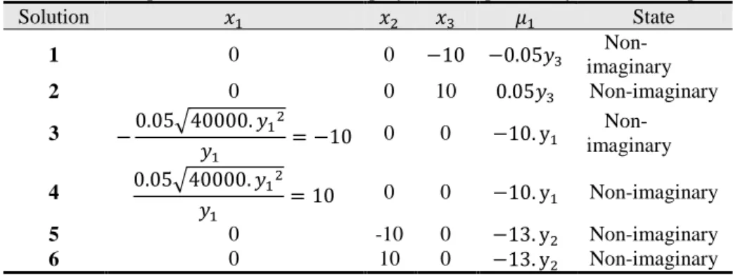
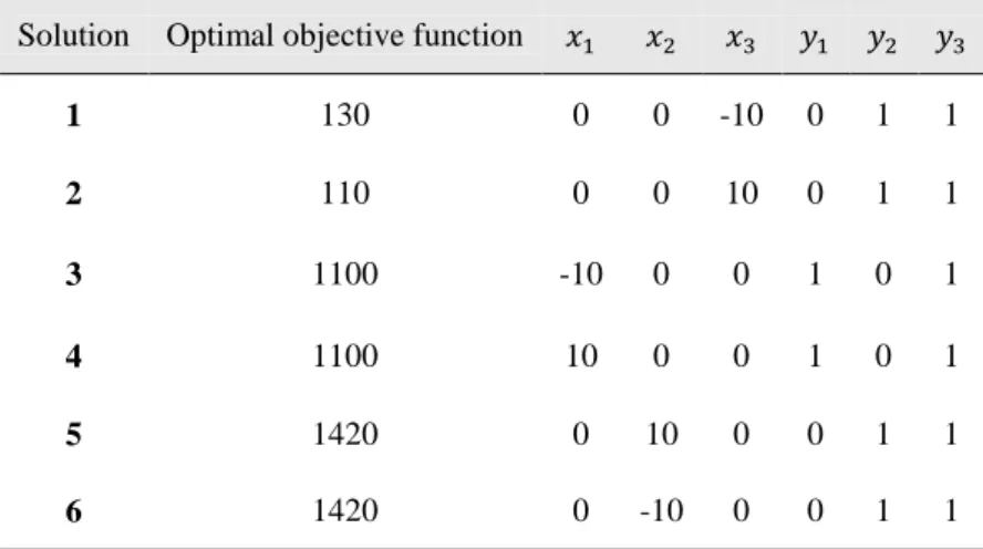
Using the conditions KKT, the system of equations (8) is formulated, and by solving this set based on the GB theory, a set of optimal candidate solutions is obtained (Table 3). Then, the objective function is reformulated for each non-imaginary solution and optimum values of them are recorded (Tables 4 and 5). By comparing the solutions in Table 5, (x₁∗ = 0 , x₂∗ = ±10 , x₃∗ = 0 , y₁∗= 0 , y₂∗ = 1 , y₃∗ = 1 , Z∗_{= 1420) is the optimal solution of the problem. Notice in this example, μ1 should be a}

non-positive because the objective function is maximized.

(8)

(

)

(

)

(

)

(

)

1 1 1 1

1

2 2 1 2

2

3 1 3

3

1 2 3

2 2 2

1 1 2 3

, ,

20 2 0

, ,

26 2 0

, , 2 0 2 0 100 0 y y y L x

x y x

x L x

x y x

x L x

y x

x

y y y

x x x

λ µ µ λ µ µ λ µ µ µ ∂ = + = ∂ ∂ = + = ∂ ∂ = − + = ∂ + + − = + +          =  −     

Table 3. The parametric solution of the polynomial equations system in example 1

State 𝜇𝜇1 𝑥𝑥3 𝑥𝑥2 𝑥𝑥1 Solution Non-imaginary −0.05𝑦𝑦3

−10 0

0

1

Non-imaginary 0.05𝑦𝑦3

10 0 0 2 Non-imaginary −10. y1

0 0 −0.05�40000._𝑦𝑦 𝑦𝑦12

1 =−10

3

Non-imaginary −10. y1

0 0 0.05�40000.𝑦𝑦12

𝑦𝑦1 = 10

4

Non-imaginary −13. y2

0 -10 0

5

Non-imaginary −13. y2

0 10 0

6

Table 4. The objective function for solutions in example 1

Objective function Solution

−100𝑦𝑦1−80𝑦𝑦2+ 210𝑦𝑦3

1

−100𝑦𝑦1−80𝑦𝑦2+ 190𝑦𝑦3

2

900𝑦𝑦1−80𝑦𝑦2+ 200𝑦𝑦3

3

900𝑦𝑦1−80𝑦𝑦2+ 200𝑦𝑦3

4

−100𝑦𝑦1+ 1220𝑦𝑦2+ 200𝑦𝑦3

5

−100𝑦𝑦1+ 1220𝑦𝑦2+ 200𝑦𝑦3

Table 5. The optimal values for each parametric solution in Example 1 𝑦𝑦3 𝑦𝑦2 𝑦𝑦1 𝑥𝑥3 𝑥𝑥2 𝑥𝑥1 Optimal objective function Solution 1 1 0 -10 0 0 130 1 1 1 0 10 0 0 110 2 1 0 1 0 0 -10 1100 3 1 0 1 0 0 10 1100 4 1 1 0 0 10 0 1420 5 1 1 0 0 -10 0 1420 6

5-2-Example 2: The MIPP problem with integer variables

This example is in the form of model (9):

(9)

(

)

{

}

1 1 1

1 1 . . 4 2 0 4 4

1, 2, ,8 Min Z x s t x y

y x x

x y = ≤ − − ≤ −         ∈  ≤ ≤ …

By considering binary variables y₁, as parameters, Lagrange function corresponding to Example 2 is constructed as follows:

𝜕𝜕𝑦𝑦(𝑥𝑥,𝜇𝜇) =𝑥𝑥1+𝜇𝜇1(𝑥𝑥1𝑦𝑦1−4) +𝜇𝜇2(𝑦𝑦1− 𝑥𝑥12(𝑥𝑥1−2)) ,

The system of equations (10) is formulated by using the KKT conditions, and Table 6 shows solutions obtained by solving this set.

(10)

(

)

(

)

(

)

(

)

1 1 2 1 2 1

1

1 1 1

2

2 1 1 1

,

1 3 2 0

4 0 2 0

y

L x

y x x

x x y

y x x

µ

µ µ µ

µ µ ∂ = + − + = ∂ − = − −      =   

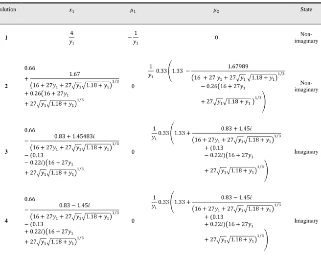
According to table 6, it is clear that the parametric solutions 3 and 4 are imaginary; hence, no investigation is needed. Solution 1 is unjustified, because for each y₁∊{1,2, … ,8}, µ₁=− 1

y1, and it is

inconsistent to the condition of non-negative µ₁ . Therefore, we just investigate Solution 2 and its corresponding objective function is as follows which is minimized at y=1. The optimal solution of example 2 is equal to (y₁∗= 1 , x₁∗= 2.2055 , Z∗= 2.2055).

𝑧𝑧𝑦𝑦= 0.66 + 1.67

�16 + 27𝑦𝑦1+ 27�𝑦𝑦1�1.18 +𝑦𝑦1�1 3⁄

+ 0.26�16 + 27𝑦𝑦1+ 27�𝑦𝑦1�1.18 +𝑦𝑦1�1 3⁄

(11)

Table 6. The solution obtained from solving polynomial parametric equations in example 2 State 𝜇𝜇2 𝜇𝜇1 𝑥𝑥1 Solution Non-imaginary 0

−_𝑦𝑦1

1 4 𝑦𝑦1 1 Non-imaginary 1

𝑦𝑦1 0.33�1.33 −

1.67989

�16 + 27𝑦𝑦1+ 27�𝑦𝑦1�1.18 +𝑦𝑦1�1 3 ⁄

−0.26�16 + 27𝑦𝑦1

+ 27�𝑦𝑦1�1.18 +𝑦𝑦1�1 3 ⁄

� 0

0.66

+ 1.67

�16 + 27𝑦𝑦1+ 27�𝑦𝑦1�1.18 +𝑦𝑦1� 1 3⁄

+ 0.26�16 + 27𝑦𝑦1

+ 27�𝑦𝑦1�1.18 +𝑦𝑦1�1 3 ⁄

2

Imaginary

1

𝑦𝑦10.33�1.33 +

0.83 + 1.45𝑖𝑖

�16 + 27𝑦𝑦1+ 27�𝑦𝑦1�1.18 +𝑦𝑦1�1 3 ⁄

+ (0.13

−0.22𝑖𝑖)�16 + 27𝑦𝑦1

+ 27�𝑦𝑦1�1.18 +𝑦𝑦1�1 3 ⁄

� 0

0.66

− 0.83 + 1.45483𝑖𝑖 �16 + 27𝑦𝑦1+ 27�𝑦𝑦1�1.18 +𝑦𝑦1�

1 3⁄

−(0.13

−0.22𝑖𝑖)�16 + 27𝑦𝑦1

+ 27�𝑦𝑦1�1.18 +𝑦𝑦1�1 3 ⁄

3

Imaginary

1

𝑦𝑦10.33�1.33 +

0.83−1.45𝑖𝑖

�16 + 27𝑦𝑦1+ 27�𝑦𝑦1�1.18 +𝑦𝑦1�1 3 ⁄

+ (0.13

+ 0.22𝑖𝑖)�16 + 27𝑦𝑦1

+ 27�𝑦𝑦1�1.18 +𝑦𝑦1�1 3 ⁄

� 0

0.66

− 0.83−1.45𝑖𝑖

�16 + 27𝑦𝑦1+ 27�𝑦𝑦1�1.18 +𝑦𝑦1�1 3 ⁄

−(0.13

+ 0.22𝑖𝑖)�16 + 27𝑦𝑦1

+ 27�𝑦𝑦1�1.18 +𝑦𝑦1� 1 3⁄

4

5-3-Example 3: The convertible MINLP problem to the MIPP problem

This example is in the form of model (12):

(12)

(

)

(

)

(

)

{

}

2 2

1 1 1 2 1 2

1 1

2 cos cos 2

. .

3 3

3, 2, 1, , 3

Min Z x y x y x y

s t x y = + − − − + + −  ≤ ≤ − −  ∈ −  …    

By replacing the first seven sentences of Taylor expansion of cosine functions of the objective function, MINLP convert into the MIPP problem as shown below:

𝑍𝑍= 3𝑥𝑥12−𝑥𝑥1 4

12 +

𝑥𝑥16

360 + 3𝑦𝑦12−

𝑦𝑦12.𝑥𝑥12

2 +

𝑦𝑦12.𝑥𝑥14

24 −

𝑦𝑦14

12 +

𝑦𝑦14.𝑥𝑥12

24 +

𝑦𝑦16

360 .

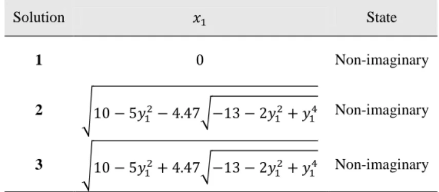
After problem conversion to MIPP and formation of the Lagrange function (which is here the same as the objective function), the KKT condition forms Set (13), and the solutions obtained are given in Table 7. By reformulating the objective function for each parametric solution in Table 7, different objective functions can be obtained (Table 8). The optimal value of the problem for each parametric solution can be seen in Table 9; the optimal solution of the problem is (x₁∗= 0, y₁∗= 0, Z∗= 0).

(13)

( )

2

1 1 1 1 1 1

1 1 1

1

. .

6 .

3 60 6 12

y

L x x x y x y x

x y x

x

∂

= − + − + +

Table 7. The obtained solution from solving polynomial parametric equations in example 3 State

𝑥𝑥1 Solution

Non-imaginary 0

1

Non-imaginary �10−5𝑦𝑦12−4.47�−13−2𝑦𝑦12+𝑦𝑦14

2

Non-imaginary �10−5𝑦𝑦12+ 4.47�−13−2𝑦𝑦12+𝑦𝑦14

3

Table 8. The objective function for each non-imaginary solution in Example 3

Objective function Solution

3𝑦𝑦12−𝑦𝑦1 4 12 +

𝑦𝑦16 360

1

24.45−8.67𝑦𝑦12−1.33y14+ 0.5y16+ 22.56�−13−2y12+ y14 −0.99𝑦𝑦12�−13−2y12+ y14

+ 0.51𝑦𝑦14�−13−2𝑦𝑦12+𝑦𝑦14

2

24.45−8.67y12−1.33y14+ 0.5y16−22.56�−13−2y12+ y14 + 0.99𝑦𝑦12�−13−2y12+ y14

−0.51y14_{�−13−2y1}2_{+ y1}4

3

Table 9. The optimal values for each parametric solution in Example 3

𝑦𝑦1 𝑥𝑥1

Optimal objective function Solution

0 0

0

1

- -

Undefined

2

- -

Undefined

3

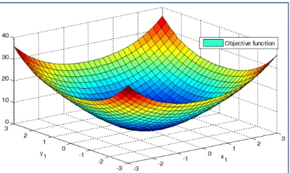
Figure 1 shows plot of the objective function of the MINLP problem (Example 3) within the specified domain of variables, assuming the continuity of y1. Obviously, in this problem, the global optimal

solution occurs at the point (x₁ = 0, y₁= 0) where the value of the objective function is zero, which is equal to the obtained solution from the proposed method.

Obviously, in the MINLP problem, the proposed method does not necessarily result in the exact global optimal solution, but because of a conversion of MINLP to the MIPP problem, an approximate of the optimal solution can be achieved, which in some problems such as Example 3, may be exactly equal to the global optimum solution.

Fig 1. Example 3, plot of the objective function, minimum value of this function occurs at the point (0, 0) and it is equal to 0

6-Performance analysis

In the previous section, three numerical examples in small dimensions were solved. Using these examples, application of the proposed solution approach was expressed. In addition, reaching the global optimal solution was ensured by use of them. In this section, a performance analysis is carried out in order to demonstrate the practical efficiency of the proposed method in the real problems and large dimensions. For this purpose, the MIPP model of a multi-products pricing problem is presented. Next, this problem is solved in various dimensions by proposed algorithm and some solvers such as BONMIN, COUENNE and BARON of GAMS software. At the end, the obtained results are reported.

6-1-MIPP model for the pricing problem

•

𝐼𝐼 Set of products

𝐷𝐷𝑖𝑖 Parameter: Maximum of demand in the market for product 𝑖𝑖

𝑀𝑀𝑖𝑖 Parameter: Minimum of allowable price for product𝑖𝑖

𝑏𝑏𝑖𝑖 Parameter: Maximum of allowable price for product𝑖𝑖

𝑐𝑐𝑖𝑖 Parameter: Production cost per unit of product𝑖𝑖

𝑐𝑐𝑀𝑀𝑐𝑐𝑖𝑖 Parameter: Production capacity of product𝑖𝑖

𝑐𝑐𝑖𝑖 Variable: Price of product𝑖𝑖

𝑑𝑑𝑖𝑖 Variable: Activated demand for product 𝑖𝑖

𝑥𝑥𝑖𝑖 Variable: Production/Supply amount of product𝑖𝑖

𝑦𝑦𝑖𝑖 Binary variable: equal to 1 if product 𝑖𝑖 is produced; 0, otherwise

•

 Objective function: maximizing of the benefit max𝑧𝑧=�(𝑐𝑐𝑖𝑖− 𝑐𝑐𝑖𝑖)𝑥𝑥𝑖𝑖

𝑖𝑖∈𝐼𝐼

 Allowable interval of price

𝑀𝑀𝑖𝑖 ≤ 𝑐𝑐𝑖𝑖 ≤ 𝑏𝑏𝑖𝑖 ∀𝑖𝑖 ∈ 𝐼𝐼

 Recursive quadratic relationship between price and demand

𝑑𝑑𝑖𝑖 =𝛽𝛽0,𝑖𝑖− 𝛽𝛽1,𝑖𝑖𝑐𝑐𝑖𝑖− 𝛽𝛽2.𝑖𝑖𝑐𝑐𝑖𝑖2 ∀𝑖𝑖 ∈ 𝐼𝐼

 Maximum variety of products supplied to the market (k is the maximum of variety)

� 𝑦𝑦𝑖𝑖 𝑖𝑖

 Other constraints

𝑥𝑥𝑖𝑖 ≤ 𝑑𝑑𝑖𝑖 ∀𝑖𝑖 ∈ 𝐼𝐼

𝑥𝑥𝑖𝑖 ≤ 𝑐𝑐𝑀𝑀𝑐𝑐𝑖𝑖.𝑦𝑦𝑖𝑖 ∀𝑖𝑖 ∈ 𝐼𝐼

Note that the objective function of the presented model and the relation between demand and price is nonlinear (as Quadratic Polynomial). The data of this problem in large dimensions have been randomly generated according to table 10.

Table 10. Randomly generated data and parameters of the MIPP pricing problem with the uniform

distribution

𝐷𝐷𝑖𝑖∈ 𝑈𝑈(1000,2000) 𝑀𝑀𝑖𝑖∈ 𝑈𝑈(5,10) 𝑏𝑏𝑖𝑖∈ 𝑈𝑈(12,25) 𝑐𝑐𝑀𝑀𝑐𝑐𝑖𝑖∈ 𝑈𝑈(800,1500) 𝑐𝑐𝑖𝑖∈ 𝑈𝑈(3,15) 𝑘𝑘= min {𝑈𝑈(1,10), |𝐼𝐼|}

𝛽𝛽0,𝑖𝑖=𝐷𝐷𝑖𝑖 𝛽𝛽1,𝑖𝑖∈ 𝑈𝑈(15,20) 𝛽𝛽2,𝑖𝑖∈ 𝑈𝑈(2,4)

6-2-The comparison of results

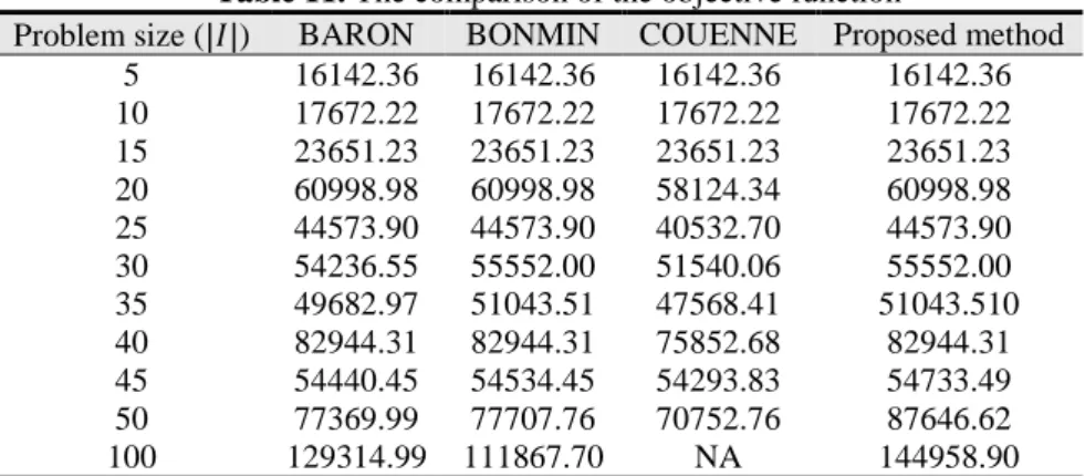
Using the data mentioned in table 10, the pricing MIPP problem has been realized in different dimensions. In the following, the results of some solvers have been compared with proposed method in the cases of the solution time and the value of objective function. Tables 11 and 12 indicate that the similar results have been obtained in the small dimensions problems. However, it was observed that by increasing the dimension of the problem, the proposed method in comparison with the other solvers presents a better objective function in the less time.

Table 11. The comparison of the objective function

Proposed method COUENNE

BONMIN BARON

Problem size (|𝐼𝐼|)

16142.36 16142.36 16142.36 16142.36 5 17672.22 17672.22 17672.22 17672.22 10 23651.23 23651.23 23651.23 23651.23 15 60998.98 58124.34 60998.98 60998.98 20 44573.90 40532.70 44573.90 44573.90 25 55552.00 51540.06 55552.00 54236.55 30 51043.510 47568.41 51043.51 49682.97 35 82944.31 75852.68 82944.31 82944.31 40 54733.49 54293.83 54534.45 54440.45 45 87646.62 70752.76 77707.76 77369.99 50 144958.90 NA 111867.70 129314.99 100

Table 12. The comparison of the solution time (minute)

Proposed method COUENNE

BONMIN BARON

Problem size (|𝐼𝐼|)

0.15 0.32 0.30 0.25 5 0.21 0.38 0.35 0.32 10 0.24 1.20 0.38 0.75 15 0.41 4.67 2.36 2.12 20 1.23 7.21 3.11 3.70 25 3.11 10.54 3.35 4.56 30 4.21 12.45 5.00 5.42 35 6.69 23.43 8.25 9.43 40 11.90 42.24 13.56 15.67 45 22.90 70.56 30.89 33.23 50 513 NA +1000 +1000 100

7-Conclusion

In this study, a specific class of MINLP problems has been discussed, and its objective function and constraints are observed to be limited to polynomials. To solve MIPP problems, we have proposed a

method that uses GB in solving the polynomial equations system. Usually, using KKT conditions to find the optimal solution of MINLP problems, a system of nonlinear equations is obtained and the analytical algorithm for solving them is not provided. However, in the MIPP problem, which is a special class of MINLP problems, the KKT condition results in a polynomial equation system (PES) where its solutions can be calculated by using some methods based on GB. In optimization problems where integer variables also exist in addition to continuous variables, one of the techniques to solve it is that, first we consider integer variables as parameters and solve a parametric continues problem and then, using a simple optimization problem, the optimal values of integer variables are calculated. In this study, this technique has been applied to solve some MIPP problems.

Although MIPP problems are not convex optimization problems, the proposed method guarantees the global optimum solution of them. Furthermore, in some class of MIPP problems that are convertible into MIPP problems in terms of Taylor's expansion of non-linear functions, using this method can approximate the optimal solution of them. In order to investigate the practical efficiency of the proposed method in the real problems, a performance analysis was conducted. The done analysis demonstrated that the proposed method in comparison with the other solvers by increasing the dimension of the problem presented a better objective function in the less time.

References

Anjos, M. F., & Vannelli, A. (2008). Computing globally optimal solutions for single-row layout problems using semidefinite programming and cutting planes. INFORMS Journal on Computing, 20(4), 611-617.

Bertacco, L., Fischetti, M., & Lodi, A. (2007). A feasibility pump heuristic for general mixed-integer problems. Discrete Optimization, 4(1), 63-76.

Boege, W., Gebauer, R., & Kredel, H. (1986). Some examples for solving systems of algebraic equations by calculating Groebner bases. Journal of Symbolic Computation, 2(1), 83-98.. 2(1): p. 83-98.

Buchberger, B. (2001). Gröbner bases and systems theory. Multidimensional systems and signal processing, 12(3-4), 223-251.

Cafaro, V. G., Cafaro, D. C., Méndez, C. A., & Cerdá, J. (2015). MINLP model for the detailed scheduling of refined products pipelines with flow rate dependent pumping costs. Computers & Chemical Engineering, 72, 210-221.2.

Cardoso, M. F., Salcedo, R. L., de Azevedo, S. F., & Barbosa, D. (1997). A simulated annealing approach to the solution of MINLP problems. Computers & chemical engineering, 21(12), 1349-1364. Chang, Y. J., & Wah, B. W. (1994, November). Polynomial programming using groebner bases. In Computer Software and Applications Conference, 1994. COMPSAC 94. Proceedings., Eighteenth Annual International (pp. 236-241). IEEE.

Crama, Y., & Rodríguez-Heck, E. (2017). A class of valid inequalities for multilinear 0–1 optimization problems. Discrete Optimization, 25, 28-47.

Deep, K., Singh, K. P., Kansal, M. L., & Mohan, C. (2009). A real coded genetic algorithm for solving integer and mixed integer optimization problems. Applied Mathematics and Computation, 212(2), 505-518.

de Lira-Flores, J., Vázquez-Román, R., López-Molina, A., & Mannan, M. S. (2014). A MINLP approach for layout designs based on the domino hazard index. Journal of Loss Prevention in the Process Industries, 30, 219-227.

Eronen, V. P., Kronqvist, J., Westerlund, T., Mäkelä, M. M., & Karmitsa, N. (2017). Method for solving generalized convex nonsmooth mixed-integer nonlinear programming problems. Journal of Global Optimization, 69(2), 443-459.

Fletcher, R., & Leyffer, S. (1994). Solving mixed integer nonlinear programs by outer approximation. Mathematical programming, 66(1-3), 327-349.

Goemans, M. X., & Williamson, D. P. (1995). Improved approximation algorithms for maximum cut and satisfiability problems using semidefinite programming. Journal of the ACM (JACM), 42(6), 1115-1145.

Gu, J., Xiao, X., & Zhang, L. (2016). A subgradient-based convex approximations method for DC programming and its applications. Journal of Industrial & Management Optimization, 12(4), 1349-1366.

Gupta, O. K., & Ravindran, A. (1985). Branch and bound experiments in convex nonlinear integer programming. Management science, 31(12), 1533-1546.

Hägglöf, K., Lindberg, P. O., & Svensson, L. (1995). Computing global minima to polynomial optimization problems using Gröbner bases. Journal of global optimization, 7(2), 115-125.

Kaur, S., Kumbhar, G., & Sharma, J. (2014). A MINLP technique for optimal placement of multiple DG units in distribution systems. International Journal of Electrical Power & Energy Systems, 63, 609-617.3.

Kim, S., & Kojima, M. (2017). Binary quadratic optimization problems that are difficult to solve by conic relaxations. Discrete Optimization, 24, 170-183.

Kirst, P., Rigterink, F., & Stein, O. (2017). Global optimization of disjunctive programs. Journal of Global Optimization, 69(2), 283-307.

Kraemer, K., Kossack, S., & Marquardt, W. (2007). An efficient solution method for the MINLP optimization of chemical processes. Computer Aided Chemical Engineering, 24, 105.8.

Lasserre, J. B. (2001). Global optimization with polynomials and the problem of moments. SIAM Journal on optimization, 11(3), 796-817.23.

Li, J., Yu, N., Liu, Z., & Shu, L. (2016). Optimal rebate strategies in a two-echelon supply chain with nonlinear and linear multiplicative demands. Journal of Industrial & Management Optimization, 12(4), 1587-1611.

Li, J., Yu, N., Liu, Z., & Shu, L. (2016). Optimal rebate strategies in a two-echelon supply chain with nonlinear and linear multiplicative demands. Journal of Industrial & Management Optimization, 12(4), 1587-1611.

Quesada, I., & Grossmann, I. E. (1992). An LP/NLP based branch and bound algorithm for convex MINLP optimization problems. Computers & chemical engineering, 16(10-11), 937-947.

Sherali, H. D., & Desai, J. (2005). A global optimization RLT-based approach for solving the hard clustering problem. Journal of Global Optimization, 32(2), 281-306.

Su, L., L. Tang, and I.E. Grossmann, Computational strategies for improved MINLP algorithms. Computers & Chemical Engineering, 2015. 75: p. 40-48.

Tokos, H., Pintarič, Z. N., & Yang, Y. (2013). Bi-objective optimization of a water network via benchmarking. Journal of cleaner production, 39, 168-179.

Westerlund, T., & Pettersson, F. (1995). An extended cutting plane method for solving convex MINLP problems. Computers & Chemical Engineering, 19, 131-136.

Yan, L., K. Shen, and S. Hu, Solving mixed integer nonlinear programming problems with line-up competition algorithm. Computers & chemical engineering, 2004. 28(12): p. 2647-2657.