SOLUTION OF SHIFF SYSTEMS BY USING DIFFERENTIAL TRANSFORM METHOD

(1)

SOLUTION OF SHIFF SYSTEMS

BY USING DIFFERENTIAL TRANSFORM METHOD

Nuran GÜZEL

1

& Muhammet KURULAY

Yildiz Technical University, Department of Mathematics, 34210-Davutpasa -Istanbul, Turkey E-mail: [email protected]

Geliş tarihi: 02.06.2008 Kabul tarihi: 21.07.2008

ÖZET

Bu çalışmada, stiff adi diferansiyel denklemleri çözmek için diferansiyel dönüşüm metodu kullanıldı ve teorisi tartışıtıldı. Metodun, lineer ve lineer olmayan diferansiyel denklem sistemlerine etkinliğini göstermek için, bazı örnekler verildi. Sayısal hesaplamalarda MAPLE bilgisayar cebiri sistemleri kullanıldı.

Anahtar Kelimeler: stiff sistem, diferansiyel dönüşüm metodu, adi diferansiyel denklemlerin

sayısal çözümü, MAPLE

ABSTRACT

In this paper, we use the differential transform method to solve stiff ordinary differential equations of the first order and an ordinary differential equation of any order by converting it into a system of differential of the order one. Theoretical considerations have been discussed and some examples were presented to show the ability of the method for linear and non-linear systems of differential equations. We use MAPLE computer algebra systems for numerical calculations [13].

Key Words: Stiff system, the differential transform method, Numerical solution of the ordinary differential

equations, MAPLE.

1.INTRODUCTION

A system of first order differential equations can be considered as: 1 1 1 2 2 1 1

( , , , )

n n n n n

y

f x y

y

f x y

y

f x y

y

′ =

⎧

⎪ ′ =

⎪

⎨

⎪

⎪ ′ =

⎩

K

M

K

(1.1)

with initial condition

0 0,

( )

,

1, 2, ,

i i

y x

=

y

i

=

_K

n

where each equation represents the first derivative of one of the unknown functions as a mapping depending on the independent variable

x

, and unknown functions

n

f

₁

, ,

_K

f

_n. Since every ordinary differential equation of order can be written as a system consisting of ordinary differential equation of order one, we restrict our study to a system of differential equations of the first order. That is,

n

f

and

y

are vector functions for which we assumed sufficient differentiability [19,12,5,16,25,2,1,21].

(2)

A special class of initial-value problems is those for which the solutions contain rapidly decaying transient terms and the numerical solution of slow smooth movements is considerably perturbed by nearby rapid solutions. Such problems are called stiff systems of differential equations. A potentially good numerical method for the solution of stiff systems differential equations must have good accuracy and some reasonably wide region of absolute stability [20]. In generally, the methods designed for non-stiff problems when applied to stiff systems of differential equations tend to be very slow and can be anomalies results in solution because stiff problems need small step lengths to avoid numerical instability. For example, when exact solution contains terms of the form , where is negative real part of a complex number problem give meaningless results. [7,11,26,27,17,24,4,29,286,20]. Because the exact solution consists of a steady-state term that does not grow significantly with

kx

e

k

x

, together with a transient term that decay rapidly to zero[7,27,17] and the error will increase since the error associated with the decreasing transient part[7].

Many algorithms are available for solving non-stiff systems [19,12,5,16,25,2,1,21] but most of these algorithms are numerically unstable for stiff systems unless the chosen step size is taken to be extremely small [7,17]. Since around 1969, numerous works have been carrying on the development of accuracy of numerical solution and efficient of methods for stiff systems because of the wide variety of applications of stiff problems occur in many areas such as chemical engineering, non-linear mechanics, biochemistry, the analysis of control system, the study of spring and damping and life sciences. Some of these are; for example, [11] discussed briefly methods of investigating the stability of particular systems and recommended implicit step methods. [26] compared two methods, GEAR and STİFF3, which were developed specifically for stiff differential equations according to accuracy of numerical solution and efficiency of method and that GEAR is the preferred algorithm for stiff differential equations. In [17], stiff differential equations are solved by Radau Methods.

Numerical methods related to stiff systems are also given in different types [11,26,27,17,24,4,29,28,6,20,22,14,15].

In the work, stiff system of differential equations is considered by differential transform method. Differential transform method can easily be applied to stiff systems of differential equations. Series coefficients can be formulated very simply.

The concept of differential transform with one-dimensional was first introduced by Zhou[30], who solved linear and non-linear initial value problems in electrical circuit analysis. Chen and Ho [9,10] proposed the method to solve eigenvalue problems and develop the basic theory of two- dimensional transform method. In the literature, different types of partial differential equations problems and differential algebraic equations problems with low index are solved by the differential transform method [30,9,10,23,8,18,3].

The method gives an analytical solution in the form of a polynomial. But, It is different from Taylor series method that requires computation the high order derivatives. The differential transform method is an iterative procedure that is described by the transformed equations of original functions for solution of differential equations.

2. THE DIFFERENTIAL TRANSFORM METHOD

The differential transform of the th derivate of function

k

y x

( )

in one dimensional is defined as follows:

0

1 ( )

( )

!

k k x x

d y x

Y k

k

dx

₌

é

ù

ê

ú

=

_ê

_ú

ë

û

(2.1)

where is original function and is transformed function and the differential inverse transform of is defined as

( )

y x

Y x

( )

Y k

(

0

)

0

( )

k

( )

k

y x

¥

x x Y

=

å

-

k

(2.2)

From (2.1) and (2.2) is defined

(

)

0 0 0

1 ( )

( )

!

k k k k _{x x}

d y x

y x

x x

k

dx

¥ = ₌

é

ù

ê

ú

=

-

_ê

_ú

ë

û

å

(2.3)

(3)

Equation (2.3) implies that the concept of the differential transformation is derived from Taylor series expansion at

x

=

x

₀. From definitions of equations (2.1) and (2.2) it is easy to obtain the basic definitions and operations of the one-dimensional differential transformation shown in Table 1. There are introduced in [9,10,23,8,18,3]. In real applications, the function

y x

( )

given in (2.3) is expressed by a finite series and equation (2.3) can be written as

(

0

)

0

( )

n k

( )

k

y x

x x Y

=

å

-

k

(2.4) where

(

₀

)

1

( )

k

( )

k n

y x

¥

x x Y

= +

=

å

-

k

is negligibly small. Table 1

The fundamental operation of one–dimensional differential transform method Original function Transformed function

( )

( ) ( )

y x =u x ±v x

( )

( ) y x =cw x

( )

/

y x

=

dw dx

( )

j

/

j

y x

=

d w dx

( )

( ) ( )

y x

=

u x v x

( )

j

y x

=

x

( )

Y k

=

U k

±

V k

( )

Y k

=

cW k

( ) (

1 ) (

1 )

Y k

=

k

+

W k

+

( ) (

1 )(

2 ...

) (

)

Y k

=

k

+

k

+

k

+

j W k

+

j

( )

k ₀

( ) (

)

r

Y k

=

∑

₌

U r V k r

−

( )

(

)

1,

0,

k

j

Y k

k

j

k

j

δ

⎧

=

−

_{= ⎨}

≠

⎩

3. Numerical Examples

The Differential transform Method applied in this study is useful in obtaining approximate solutions of stiff ordinary differential equations of first order and an ordinary differential equation of any order. We illustrate it by the following examples using MAPLE computer algebra systems [13].

Example 1. We consider the following differential equation system[15]

2 1 1 2 1 2 2

1002

1000

(1

)

2

y

′ = −

+

′ = −

+

(3.1)

with initial condition

1

(0) 1

y

=

and

y

₂

(0) 1

=

. The exact solution is

_{y x}

₁

( )

₌

_e

−2x_and

2

( )

x

y x

=

e

− .

By using the basic properties of differential transform method from table 1 and taking the transform of Eqs. (3.1) we can obtain that

(4)

(

_{) ( )}

( ) (

)

(

_{) ( )}

( ) (

)

1 1 2 0 2 1 2 2 2 0

1

1 1002. ( ) 1000.

1

1 ( )

( )

1

k r k r

Y k

Y r Y k r

k

Y k

Y r Y k r

k

= =

⎛

⎞

+ =

_⎜

−

+

−

_⎟

+ ⎝

⎠

⎛

⎞

+ =

_⎜

−

+

−

_⎟

+ ⎝

⎠

∑

2

m

(3.2)

Substitute

k

=

0,1,...,

into (3.2), series coefficients can be obtained that

1 1 1 1 2 2 2 2

(2) 2,

4

8 (7)

31 (2)

,

(7)

5 Y

Y

=

1 1 1 1 1 2 2 2 2 2

4

2

4 (1)

2,

(3)

,

(4)

,

(5)

,

3

15

2

4 (6)

,

(8)

,

(9)

45

5

315 2835

1

1 (1)

1,

(3)

,

(4)

,

(5)

,

2

6

24

720

1

1 (6)

,

(8)

,

(9)

720

040 40320

362880

Y

= −

=

= −

−

=

= −

=

= −

−

=

= −

By substituting the values of

Y k and Y k

₁

( )

₂

( )

into (2.2), we obtain

y x

₁

( )

and

y x

₂

( )

as

( )

2 3 4 5 6 7 8 1

4

2

4

8

2

4 1 2

2

3

15

45

315

315 2835

9

y x

= −

x

+

x

−

x

+

x

−

x

+

x

−

x

+

x

−

x

( )

2 3 4 5 6 7 8 2

1

2

6

24

720

720 5040

40320

362880

y x

= − +

x

−

x

+

x

−

x

+

x

−

x

+

x

−

x

9

The numerical results are illustrated in table 2 and 3.

Table 2.

Comparison of theoretical and numerical values of

y

₁in example 1.

t

Theoretical (

y

₁) Numerical(

y

₁) Error 0.1 0.8187307531 0.8187307532 0.0000000001 0.2 0.6703200460 0.6703200461 0.0000000001 0.3 0.5488116361 0.5488116345 0.0000000016 0.4 0.4493289641 0.4493289365 0.0000000276 0.5 0.3678794412 0.3678791888 0.0000002524 0.6 0.3011942119 0.3011926747 0.0000015372 0.7 0.2465969639 0.2465899006 0.0000070633 0.8 0.2018965180 0.2018701030 0.0000264150 0.9 0.1652988882 0.1652144772 0.0000844110 1.0 0.1353352832 0.1350970018 0.0002382814

(5)

Table 3.

Comparison of theoretical and numerical values of the

y

₂in example 1.

t

Theoretical (

y

₂) Numerical(

y

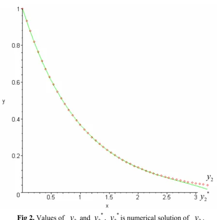
₂) Error 0.1 0.9048374180 0.9048374181 0.0000000001 0.2 0.8187307531 0.8187307532 0.0000000001 0.3 0.7408182207 0.7408182206 0.0000000001 0.4 0.6703200460 0.6703200461 0.0000000001 0.5 0.6065306597 0.6065306595 0.0000000002 0.6 0.5488116361 0.5488116345 0.0000000016 0.7 0.4965853038 0.4965852966 0.0000000072 0.8 0.4493289641 0.4493289365 0.0000000276 0.9 0.4065696597 0.4065695710 0.0000000887 1.0 0.3678794412 0.3678791887 0.0000002525

Fig 1. Values of

y

1 and * 1

(6)

2

y

* 2

y

Fig 2. Values of

y

₂ and

y

₂*,

y

₂*is numerical solution of

y

₂.

Example 2. Let us consider following system of differential equation[15]

1 1 2 3 1 2 1 2 3 2 3 1 2 3 3

20

0.25 19.75 , (0) 1,

20

20.25 0.25 , (0) 0,

20

19.75 0.25 , (0)

1. y

y

′ = −

−

=

′ =

−

+

=

′ =

−

= −

(3.3) with initial values

( )

1

0

1

2

0

3

0 y

=

y

=

y

= −

1 / 2,

)]/ 2.

The analytic solution of the problem is 1/ 2 20 1 1/ 2 20 2 1/ 2 20 3

[

(cos(20 ) sin(20 ))]

[

(cos(20 ) sin(20 ))]/ 2,

[

(cos(20 ) sin(20 )

t t t t t t

y

e

t

y

e

t

y

e

t

− − − − − −

=

+

=

−

= −

+

−

If we apply differential transform method to the given equation system, it is obtained that

(

_{) ( )}

(

( )

)

(

_{) ( )}

(

( )

(

_{) ( )}

)

( )

(

)

1 1 2 2 1 2 3 1 2

1

20

0.25

19.75

1

1 20 ( ) 20.25 ( ) 0.25

1

1 20 ( ) 19.75 ( ) 0.25

1 Y k

Y k

k

Y k

k

Y k

k

+ =

−

+

+ =

−

+

+ =

−

+

3 3 3 (3.4)

(7)

For

k

=

0,1,...,

m

Y k Y k Y k

₁

( ) ( ) ( )

,

₂

,

₃ coefficients can be calculated from (3.4) as 1 1 1 1 1 1 1 1 1 2 2 2

1 3199

85333

3413333

1 (1)

,

(2)

,

(3)

,

(4)

,

(5)

,

4

16

32

256 7680

3640888889

2621440000001

104857600000001

1 (6)

, (7)

, (8)

,

(9)

10240

1290240

315 371589120

79 3199

1 (1)

,

(2)

,

(3)

4

16

96 Y

Y

= −

=

= −

=

= −

=

= −

=

= −

₂ ₂ 2 2 2 2 3 3 3 3 3

10240001

273066667

,

(4)

,

(5)

,

768 2560

3640888889

1 4993219047619

838860799999

(6)

,

(7)

,

(8)

,

(9)

10240

1290240

983040

371589120

81 3201

1 3413333

819199999

(1)

,

(2)

,

(3)

,

(4)

,

(5)

4

16

96

256

7 Y

Y

=

= −

=

= −

=

= −

=

= −

3 3 3 3

,

680 32767999999

1 104857600000001

27962026666667

(6)

,

(7)

,

(8)

,

(9)

92160

1290240

20643840

123863040

Y

=

Y

=

Y

= −

Y

= −

Y k

₁

( )

,

Y k Y k

₂

( ) ( )

,

₃ into (2.2), we obtain

y x

₁

( )

,

y x

₂

( )

and

y x

₃

( )

as

( )

2 3 4 5 1

1 3199

85333

3413333

1 3640888889

1 ...

4

16

32

256 7680

10240

y x

= −

x

−

x

+

x

−

x

−

x

+

x

6

( )

2 3 4 5 2

79 3199

1 10240001

27306667

3640888889

...

4

16

96

768 2560

10240

6

y x

=

x

−

x

−

x

+

x

−

x

+

x

( )

2 3 4 5 6 3

81 3201

1 3413333

819199999

32767999999

1 ...

4

16

96

256 7680

92160

y x

= − +

x

−

x

+

x

+

x

−

x

+

x

.

The numerical results are illustrated in table 3, 4 and 5.

Table 4.

y

₁in example 2.

t

Theoretical (

y

₁) Numerical(

y

₁) Error 0.1 0.9476815826 0.9476815825 0.0000000001. 0.2 0.9968025985 0.9968025984 0.0000000001. 0.3 0.9935823806 0.9935823807 0.0000000001. 0.4 0.9893856850 0.9893856852 0.0000000002. 0.5 0.9842872353 0.9842872356 0.0000000003 0.6 0.9783588395 0.9783588396 0.0000000001 0.7 0.9716694173 0.9716694174 0.0000000001 0.8 0.9642850327 0.9642850329 0.0000000002 0.9 0.9562689318 0.9562689318 0.0000000000 1.0 0.9476815826 0.9476815825 0.0000000001

(8)

Table 5.

y

₂in example 2.

t

Theoretical (

y

₂) Numerical(

y

₂) Error 0.1 0.0338613302 0.0338613302 0.0000000000 0.2 0.0665062521 0.0665062520 0.0000000001 0.3 0.0979389656 0.0979389656 0.0000000000 0.4 0.1281662413 0.1281662413 0.0000000000 0.5 0.1571972304 0.1571972304 0.0000000000 0.6 0.1850432835 0.1850432834 0.0000000001 0.7 0.2117177754 0.2117177754 0.0000000000 0.8 0.2372359366 0.2372359366 0.0000000000 0.9 0.2616146929 0.2616146930 0.0000000001 1.0 0.2848725110 0.2848725109 0.0000000001 Table 6.

y

₃in example 2.

t

Theoretical (

y

₃) Numerical(

y

₃) Error 0.1 0.9652663858 0.9652663857 0.0000000001 0.2 0.9317499408 0.9317499409 0.0000000001 0.3 0.8994464644 0.8994464644 0.0000000000 0.4 0.8683491855 0.8683491855 0.0000000000 0.5 0.8384489520 0.8384489520 0.0000000000 0.6 0.8097344126 0.8097344126 0.0000000000 0.7 0.7821921922 0.7821921921 0.0000000001 0.8 0.7558070592 0.7558070590 0.0000000002 0.9 0.7305620874 0.7305620874 0.0000000000 1.0 0.7064388095 0.7064388093 0.0000000002

Example 3. Consider following system [15]

' 1 1 2 ' 2 1 2 ' 3 1 2

21

19

20

19

21

20

40

3 3 3

y

= −

+

−

=

−

+

=

−

+

(3.5) with initial values

( )

1

0

1

2

0

3

0

(9)

The analytic solution of the problem is

( )

(

)

( )

(

)

( )

(

)

2 40 1 2 40 2 2 40 3

cos 40

sin 40

2 cos 40

sin 40

2 cos 40

sin 40

2.

t t t t t t

y

e

t

y

e

t

y

e

t

− − − − − −

⎡

⎤

=

_⎣

+

_⎦

⎡

⎤

=

_⎣

−

_⎦

⎡

⎤

= −

_⎣

+

−

_⎦

By using the basic properties of differential transform method and taking the transform of Eqs. (3.5) we have

(

_{) ( )}

(

( )

)

(

_{) ( )}

(

( )

(

_{) ( )}

)

( )

(

)

1 1 2 2 1 2 3 1 2

1

21

19

20

1

1 19 ( ) 21 ( ) 20

1

1 40 ( ) 40 ( ) 40

1 Y k

Y k

k

Y k

k

Y k

k

+ =

−

+

−

+

+ =

−

+

+ =

−

+

3 3 3

.

(3.6)

For

k

=

0,1,...,

m

Y k Y k Y k

₁

( ) ( ) ( )

,

₂

,

₃ coefficients can be calculated from (3.6) as

1 1 1 1 1 1 1 1 1 2 2 2 2 2 2

63998

2 (1)

1,

(2)

799,

(3)

,

(4)

213333,

(5)

,

3

1 113777778

27306666668

409600000001

2 (6)

, (7)

, (8)

,

(9)

5

105

315 2835

640001

2 (1)

1,

(2) 801,

(3)

21334,

(4)

,

(5)

,

3

15 (6)

Y

= −

=

= −

=

= −

=

= −

=

= −

=

= −

5

2 2 2 3 3 3 3 3 3 3 3 3

1023999998

819999996

45511111111

2 ,

(7)

,

(8)

,

(9)

45

315

35 2835

1280000

20480000

(1) 80,

(2)

1600,

(3) 0,

(4)

,

(5)

,

3

3 409600000

163840000000

13107200000000

(6)

,

(7) 0,

(8)

,

(9)

9

63

567 Y

Y

=

= −

=

= −

=

= −

=

= −

=

Y k

₁

( )

,

Y k Y k

₂

( ) ( )

,

₃ into (2.2), we obtain

y x

₁

( )

,

y x

₂

( )

and

y x

₃

( )

as

( )

2 3 4 5 1

63998

2 113777778

1

799 213333

...

3

15

5 y x

= − −

x

+

x

− −

x

−

x

+

x

6

( )

2 3 4 5 2

640001

2 1023999998

801 21334

...

3

15

45

6

y x

= − +

x

−

x

+

x

−

x

−

x

( )

2 4 5 3

1280000

20480000

409600000

1 80

1600

...

3

9

6

y x

= − +

x

−

x

−

x

−

x

+

x

(10)

Table 7.

y

₁in example 3.

t

Theoretical(

y

₁) Numerical(

y

₁) Error 0.1 0.9959322154 0.9959322153 0.0000000001 0.2 0.9876494697 0.9876494696 0.0000000001 0.3 0.9757613240 0.9757613237 0.0000000003 0.4 0.9608307308 0.9608307306 0.0000000002 0.5 0.9433749893 0.9433749894 0.0000000001 0.6 0.9238669934 0.9238669939 0.0000000005 0.7 0.9027367174 0.9027367204 0.0000000030 0.8 0.8803729025 0.8803729145 0.0000000120 0.9 0.8571248954 0.8571249329 0.0000000375 1.0 0.8333046046 0.8333047113 0.0000001067

Example 4. We consider a system representing a nonlinear reaction was taken from Hull [21].

1 1 2 2 1 2 2 3 2

,

.

dy

y

dt

dy

y

dt

dy

y

dt

= −

=

−

=

(3.7)

The initial conditions are given by

y

₁

(0) 1, (0) 0

=

y

₂

=

and

y

₃

(0) 0

=

. By taking the transform of Eqs (3.7) we have

(

)

₍

_{) ( )}

(

_{) ( )}

(

_{) ( )}

1 1 2 1 2 2 0 3 2 2 0

1

1 ( )

( ) (

1

1 ( ) (

)

1

k r k r

Y k

k

Y k

Y r Y k r

k

Y k

Y r Y k r

k

= =

+ = −

+

⎛

⎞

+ =

_⎜

−

+ ⎝

⎠

+ =

−

+

∑

)

_⎟

(3.8)

For

k

=

0,1,...,

m

Y k Y k Y k

₁

( ) ( ) (

,

₂

,

₃

)

coefficients can be calculated from (3.8) and substituting these values into (2.2), we have

y x

₁

( )

,

y x

₂

( )

and

y x

₃

( )

that

( )

2 3 4 5 6 7 8 1

1

2

6

24

120

720 5040

40320

362880

9

y x

= − +

x

−

x

+

x

−

x

+

x

−

x

+

x

−

x

( )

2 3 4 5 6 7 8 2

1

5

1

71

19 1469

329

2

6

24

40

720 1008

40320

17280

9

y x

= −

x

−

x

+

x

+

x

−

x

+

x

+

x

−

x

( )

3 4 5 6 7 8 3

1

7

47

7

691

3

4

60

72 2520

192 36288

y x

=

x

−

x

−

x

+

x

−

x

−

x

+

x

9

(11)

5. CONCLUSION

The differential transform method has been applied to the solution of stiff systems of differential equations. The numerical examples have been presented to show that the approach is promising and the research is worth to continue in this direction. Using the differential transform method, the solution of the stiff systems of differential equations can be obtained in Taylor’s series form. All the calculations in the method are very easy. The calculated results are quite reliable and are compatible with many other methods such as Pade Approximation that we studied in [15]. The method is very effective to solve most of differential equations system.

REFERENCES

[1] Amodio,P., Mazzia F., Numerical solution of differential-algebraic equations and Computation of consistent initial/boundary conditions. Journal of Computational and Applied Mathematics. 87(1997) 135-146.

[2] Ascher, UM., Petzold, LR., Computer Methods for Ordinary Differential Equations and Differential-Algebraic Equations, SIAM, (1998), Philadelphia.

[3] Ayaz, F., On the two dimentional differential transform method, Applied Mathematics and Computation, 143, (2003), 361-374.

[4] Blue , JL., Gummel, HK., Rational approximations to matrix exponential for systems of stiff differential equations, Journal of Computational Physics, Vol.5,Issue 1,( 1970),70-83.

[5] Brenan, K.E., Campbell, S.L., Petzold L.R., Numerical solution of Initial-value problems in Differential-Algebraic Equations, North-Holland, Amsterdam ,(19899.

[6] Brydon D., Pearson J., Marder M., Solving Stiff Differential Equations with the Method of Patches, Journal of Computational Physics 144,(1998)280-298.

[7] Burden,RL., Faires J.D., Numerical Analysis, Fifth Edition, PWS Publishing Company,(1993),Boston. [8] Chen, C.L, Liu, Y.C., Solution of Two-Point Boundary-Value Problems Using the Differential

Transformation Method, Journal of Optimization and Applications,Vol.99,No.1, Oct.(1998),23-35.

[9] Chen,C.K., Ho,S.H., Application of differential transformation to eigenvalue problems, Appl. Math. Comp., 79, (1996), 173-188.

[10] Chen,C.K., Ho,S.H., Solving partial differential equations by two dimensional differential transform method, Applied Mathematics and Computation, 106, (1999), 171-179.

[11] Cooper,GJ., The numerical solution of stiff differential equations, FEBS Letters, Vol.2, Supplement 1, March 1969, S22-S29.

[12] Corliss G. And Chang Y. F., Solving Ordinary Differential Equations Using Taylor Series, ACM Trans. Math. Soft. 8(1982), 114-144.

[13] Frank G., MAPLE V:CRC Press Inc., 2000 Corporate Blvd., N.W., Boca Raton, Florida 33431, (1996). [14] Garfinkel, D.,Marbach, C.B, Stiff Differential Equations, Ann. Rev. BioPhys. Bioeng. 6,( 1977),525-542. [15] Guzel, N., Bayram,M., On the numerical solution of stiff systems, Applied Mathematics and Computation,

170, (2005), 230-236.

[16] Hairer, E. and Wanner, G., Solving Ordinary Differential Equations II: Stiff and Differential-Algebreis Problems, Springer-Verlag,( 1991).

[17] Hairer,E., Wanner,G., Stiff differential equations solved by Radau Methods, Journal of Computational and Applied Mathematics, 111, 1999,93-111.

[18] Hassan,I.H.Abdel-Halim, Different applications for the differential transformation in the differential equations, Applied Mathematics and Computation, 129, (2002), 183-201.

(12)

[19] Henrici, P., Applied Computational Complex Analysis, Vol.1, John Wiely&Sons, New York, Chap.1, (1974).

[20] Hojjati,G., Ardabili MYR., .Hosseini, SM, Newsecond derivative multistep methods for stiff systems, Applied Mathematical Modelling,30,(2006)466-476.

[21] Hull ,TE., Enright,WH., Fellen BM., Sedgwick AE., Comparing numerical methods for ordinary differential equations, SIAM J, Numer.Anal. 9 (1972) 603.

[22] Jackiewicz, Z., Implementation of DIMSIMs for stiff differential systems, Applied Numerical Mathematics 42 (2002) 251-267.

[23] Jang,C. Chen C.L.,Liu,YC. On Solving The initial-value problems using the differential transformation method, Applied Mathematics and Computation, 115,(2000), 145-160.

[24] Preiser,DL. , A Class of nonlinear multistep A-stable numerical methods for solving stiff differential equations, Computer&Mathematics with Applications,Vol.4,Issue 1, 1978,43-51.

[25] Press, WH., Flannery BP., Teukolsky S.A., Vetterling W.T., Numerical Recipes, Cambridge University Press,(1988), Cambridge.

[26] Rangaiah,G.P., Comparson of two algorithms for solving STIFF differential equations, Computer&Structures, Vol. 20, Issue 6,(1985), 915-920.

[27] Sottas,G., Rational Runge-Kutta methods are not suitable for stiff systems of ODEs, Journal of Computational and Applied Mathematics, Vol.10, Issue 2, April 1984,169-174.

[28] Tripathy,SC., S. and Balasubramanian, R., Semi-İmplicit Runge-Kutta methods for power system transient stability studies, International journal of Electrical Power&Energi Systems,Vol.10,Issue 4,Oct 1988,253-259.

[29] Ypma,T.J., Relaxed Newton-Like Methods for stiff differential systems, Journal of Computational and Applied Mathematics, Vol.16, Issue 1, September 1986,95-103.

[30] Zhou,JK., Differential Transformation and Its Applications for Electrical Circuits,Huazhong Un.Press,Wuhan,China,(1986).